The resolved star formation history of M51a through successive Bayesian marginalization

Abstract

We have obtained the time and space-resolved star formation history (SFH) of M51a (NGC 5194) by fitting GALEX, SDSS, and near infrared pixel-by-pixel photometry to a comprehensive library of stellar population synthesis models drawn from the Synthetic Spectral Atlas of Galaxies (SSAG). We fit for each space-resolved element (pixel) an independent model where the SFH is averaged in 137 age bins, each one 100 Myr wide. We used the Bayesian Successive Priors (BSP) algorithm to mitigate the bias in the present-day spatial mass distribution. We test BSP with different prior probability distribution functions (PDFs); this exercise suggests that the best prior PDF is the one concordant with the spatial distribution of the stellar mass as inferred from the near infrared images. We also demonstrate that varying the implicit prior PDF of the SFH in SSAG does not affects the results. By summing the contributions to the global star formation rate of each pixel, at each age bin, we have assembled the resolved star formation history of the whole galaxy. According to these results, the star formation rate of M51a was exponentially increasing for the first 10 Gyr after the Big Bang, and then turned into an exponentially decreasing function until the present day. Superimposed, we find a main burst of star formation at $t\approx$ 11.9 Gyr after the Big Bang.

1 Introduction

Modern multiwavelength and integral field unit (IFU) data provide unprecedented information that can help uncover essential aspects of galaxy formation and evolution. Resolved studies of galaxy properties on a pixel-by-pixel (e.g. Zibetti, Charlot, & Rix, 2009; Mentuch Cooper et al., 2012; Sorba & Sawicki, 2015; Díaz-García et al., 2015; Martínez-García et al., 2017; Abdurro’uf, 2017), or spaxel-by-spaxel basis (e.g. González Delgado et al., 2014, 2015, 2016; Cano-Díaz et al., 2016; Ibarra-Medel et al., 2016; de Amorim et al., 2017) have become standard practice in modern investigations. These methods commonly use state-of-the-art stellar population synthesis (SPS) models to compare with observations. Martínez-García et al. (2017) introduced a novel and sophisticated Bayesian fitting method to remove a bias originated from traditional fitting techniques to pixel-by-pixel photometry. The bias consists in an apparent spatial coincidence between the resolved stellar mass surface density (or mass-map) and the observed dust lanes (produced by internal galaxy extinction), resulting in an illusory filamentary spatial distribution for the mass. In this work we aim to describe an ancillary output of the Martínez-García et al. (2017) mass-map method, related to the recovery of the star formation history (SFH) of a disk galaxy. The novel method determines the resolved SFH by fitting a library of SPS models to UV, optical, and near infrared (NIR) photometry on a pixel-by-pixel basis. The recent star formation rate (SFR, $\Psi$) of a galaxy can be inferred from its ultraviolet (UV) continuum luminosity. However, $\Psi_{\rm UV}$ may exceed other $\Psi$ indicators if the extinction is overestimated due to the underlying Balmer absorption (Rosa-González et al., 2002). Salim et al. (2007, 2016) have shown that $\Psi$ can be better estimated from spectral energy distribution (SED) fits that include the optical and NIR ranges besides the UV. We have included these wavelength ranges in our method and applied it to the Whirlpool galaxy, aka M51a. The results and their implications are shown in this paper.

Throughout this work we adopt the cosmological parameters of Bennett et al. (2014), and use the cosmological calculator of Wright (2006) where necessary.

2 Observational data

For this investigation we use far and near ultraviolet ($FUV$ and $NUV$, respectively) imaging from the GALEX Ultraviolet Atlas of Nearby Galaxies (Gil de Paz et al., 2007), $g$- and $i$-band optical data from the 12th Sloan Digital Sky Survey (SDSS) data release (Alam et al., 2015), and the NIR $K_{s}$ mosaic from Gonzalez & Graham (1996). The latter was photometrically calibrated using the Two Micron All Sky Survey (2MASS, Skrutskie et al., 2006).

We registered the images to the spatial resolution of the $FUV$ image (which has a plate scale of $1.5\arcsec$ pixel^-1) using the world coordinate system (WCS) information. We noticed a spatial mismatch between the structural features and star forming regions of the $NUV$ and the $g$ image that is not present when the $FUV$ and $g$ images are compared. We correct for this discrepancy by registering the $NUV$ to the $FUV$ image based on the features they have in common. Foreground stars were removed by replacing their pixels with values similar to the background-subtracted ‘sky’.

The $FUV$ and $NUV$ images have a point-spread function (PSF) with a full width at half maximum (FWHM) a factor of $\sim$4 larger than SDSS frames. In order to get a common PSF for all our data, we use the 2017 version of the convolution kernels of Aniano et al. (2011).

To increase the signal to noise (S/N) ratio of the outer disk pixels in the $NUV$ frame, we adopt the Adaptsmooth code of Zibetti (2009). We require a minimum S/N ratio per pixel of 20, a maximum smoothing radius of 10 pixels, and assume background-dominated noise. The code produces a ‘smoothing mask’, which contains the smoothing radius (in pixels) at each position. We then use this output mask in a second run of Adaptsmooth on the $FUV$, $g$, $i$, and $K_{s}$ data. Subsequently, we compute the 1-$\sigma_{\rm mag}$ error, on a pixel-by-pixel basis, for each band, following Martínez-García et al. (2017, their section 4). We assume zero-point errors of $\sigma_{\rm calib}\approx 0.15$ mag for the $FUV$ and $NUV$ data, $\sigma_{\rm calib}\approx 0.01$ mag for the SDSS images, and $\sigma_{\rm calib}\approx 0.033$ mag for the $K_{s}$ mosaic.

We end up with $\sim 8\times 10^{4}$ data pixels for each image that can be fitted with our method. We assume a distance to M51a of $8.58\pm 0.10$ Mpc (McQuinn et al., 2016), which results in a physical scale of $\sim 62$ pc pixel^-1. Taking into account the PSF of the $NUV$ band (FWHM$\sim 5.25\arcsec$), the recovered physical scale is $\sim 0.22$ kpc. Optical and NIR Galactic extinction was taken into account by using the Schlafly & Finkbeiner (2011) recalibration of Schlegel et al. (1998) with $R_{V}=3.1$. $NUV$ and $FUV$ Galatic extinction was corrected as in Peek & Schiminovich (2013, their equations 4 and 7, respectively).

3 Analysis

From the observational data we construct the $(FUV-NUV)$, $(NUV-g)$, $(g-i)$, and $(i-K_{s})$ colour images. These are used as input to the Bayesian Successive Priors (BSP) method of Martínez-García et al. (2017). Briefly, the BSP algorithm consists of three iterations to produce a stellar surface density mass-map consistent with the NIR spatial structure of a disk galaxy (see, e.g., Rix & Rieke, 1993). In the first iteration, a maximum-likelihood estimate is used to maximise the probability $P\propto\exp\left(-\frac{\chi^{2}}{2}\right)$, where $\chi$ represents the difference between the observed colours and the predicted colours of the SPS library, weighted by their errors. The second iteration assumes a constant stellar mass-to-light ratio $\Upsilon_{*}$, in the NIR, for the entire disk. The third iteration deals with the resolved elements (pixels) that cannot be adequately fitted with a constant $\Upsilon_{*}^{\rm NIR}$. In this manner, the second and third iterations introduce a prior probability distribution function (PDF) to account for the observed NIR spatial structure; the best fit model is the one that maximises the probability

$$~{}P(\Upsilon_{*}\mid C)\propto\exp\left(-\frac{\chi^{2}}{2}\right)\exp\left(-\frac{1}{2}\left[\frac{\Upsilon_{*}^{\rm prior}-\Upsilon_{*}}{\sigma_{\Upsilon_{*}}}\right]^{2}\right),$$ (1)

where $C$ represents the observed colours for a certain stellar population, and $\sigma_{\Upsilon_{*}}\approx\sigma_{\rm mag}\Upsilon_{*}^{\rm prior}$. We obtain the resolved stellar mass-map of M51a from the $(FUV-NUV)$, $(NUV-g)$, $(g-i)$, and $(i-K_{s})$ colours, hence $N_{\rm colours}=4$, and the mass-to-light ratio $\Upsilon^{K_{s}}_{*}$ in the $K_{s}$ band. We find that, as seen in Figure 1, the inclusion of the UV bands in the first iteration fits does not remove the bias and the spatial structure described by Martínez-García et al. (2017). Thus, the application of the full BSP algorithm is justified in this work. We should also mention that although BSP iteration number 2 assumes a prior $\Upsilon^{K_{s}}_{*}$ that is a constant for the entire disk, the posterior $\Upsilon^{K_{s}}_{*}$ is not necessarily univariate (for both BSP iterations number 2 and 3). This is shown in Figure 2, where we plot a 2-D histogram of the posterior $\Upsilon^{K_{s}}_{*}$ after BSP iterations number 2 and 3, for all the fitted pixels of M51a (see also Martínez-García et al., 2017, their figure 11, panel d).

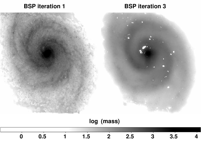
Figure 1: Left: M51a stellar mass-map derived with the BSP algorithm, iteration number 1, based on $(FUV-NUV)$, $(NUV-g)$, $(g-i)$ and $(i-K_{s})$ colours, and $K_{s}$ mass-to-light ratio, $\Upsilon_{*}^{K_{s}}$. Right: same as left for BSP iteration number 3. Mass in M_☉ pc^-2.

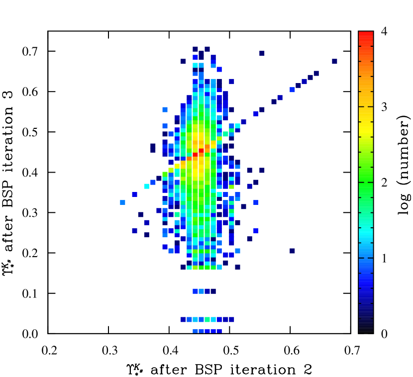
Figure 2: 2D histogram of the posterior $\Upsilon_{*}^{K_{s}}$ of M51’s pixels, after BSP iterations number 2 and 3, in the $x$- and $y$-axis, respectively.

For this research we adopt an SPS library consisting of $\sim 7\times 10^{4}$ templates extracted from the 2017 version of the Synthetic Spectral Atlas of Galaxies (SSAG-2017 hereafter). In the SSAG-2017, the stellar metallicity is distributed uniformly between $0.006\leqq Z/Z_{\sun}\leqq 3.53$. The effects of dust are computed with the model of Charlot & Fall (2000); the dust parameters follow Gaussian PDFs. The SSAG spectra are convolved with a Gaussian filter to mimic the effects of the stellar velocity dispersion. The adopted stellar initial mass function (IMF) is Chabrier (2003). The SSAG uses an SFH recipe proposed by Chen et al. (2012). This SFH prescription consists of a first episode of star formation (SF) characterised by an exponentially declining event. For all templates the beginning of star formation is determined by the parameter T_form, in look-back time units. Also, in the SSAG-2017, 55 per cent of the galaxies experience a superimposed burst of SF of finite duration and random amplitude (cf. Magris et al., 2015, their Appendix B). Bursts are onset at any time in the past, but are constrained such that 15 per cent of the total galaxies present a burst in the last 2 Gyr. Some galaxies may also undergo a ‘truncation’ event, at which $\Psi$ starts to decline at a faster rate than before. It is assumed that 30 per cent of the galaxies experience this truncation event, and that 35 per cent of the truncation events occur over the last 2 Gyr (this corresponds to 10 per cent of the total galaxies). As an example, in Figure 3 we show the SFHs for two SSAG templates.

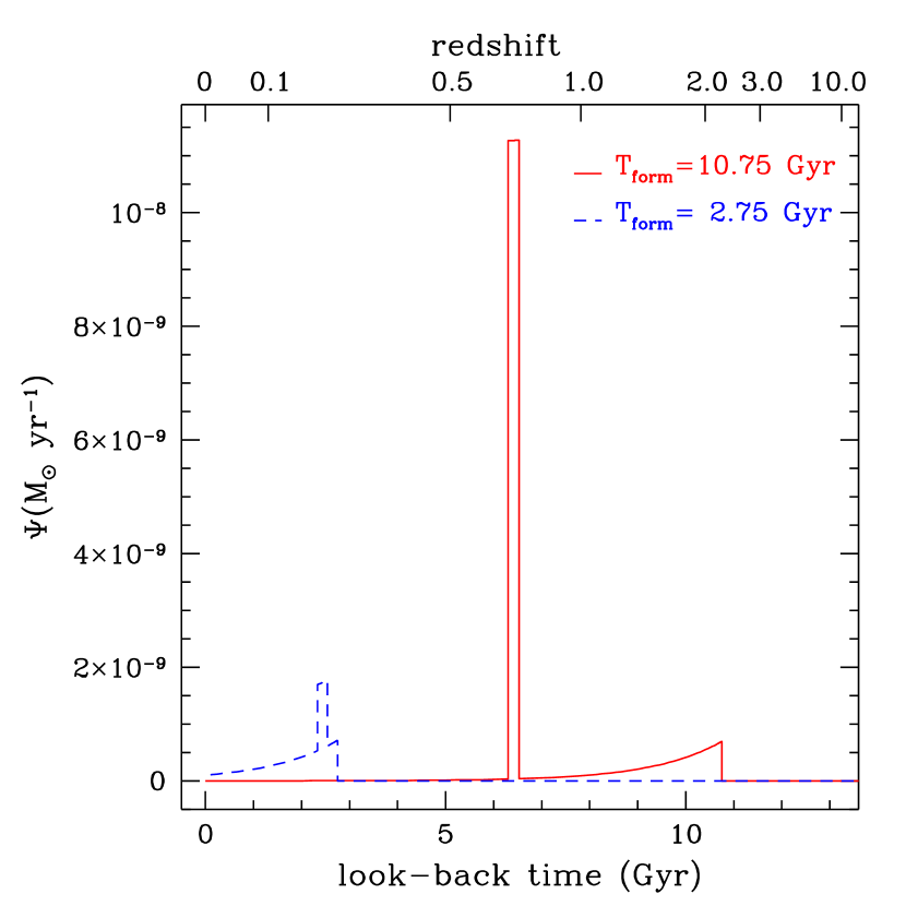
Figure 3: SFHs for two different SSAG templates. Solid red line: the galaxy starts forming stars at T_form=10.8 Gyr ago, and experiences a burst after 4.2 Gyr, lasting 0.2 Gyr. Dashed blue line: T_form = 2.8 Gyr, burst starts after 0.2 Gyr, lasting 0.2 Gyr. Star formation rates, $\Psi$, scale with galaxy mass (Bruzual & Charlot, 2003).

The BSP algorithm produces a mass-map by allocating a probability to each template in the corresponding SPS library. Each template has its own set of parameters, e.g., metallicity, or dust content. In this sense, we obtain a resolved map not only for the stellar mass, but also for each parameter in the library, including the SFH.

For the present analysis, the SFH for each template is averaged in age bins of 100 Myr, for a total of 137 age bins between today and $\sim 0.02$ Gyr after the Big Bang. The average SFR for each bin is then

$$\langle\Psi(t_{L})\rangle=\frac{\int_{t_{L}}^{t_{L}+t_{\rm bw}}\Psi(t^{\prime}){\rm d}t^{\prime}}{t_{\rm bw}},$$ (2)

where time $t_{L}$ is the look-back time of the bin’s boundary (the side closest to $t_{L}=0$, i.e., today), and $t_{\rm bw}=10^{8}$ yr is the corresponding bin width. We calculate $\langle\Psi(t_{L})\rangle$ for each pixel and then sum over all pixels to obtain the global value

$$~{}\langle\Psi(t_{L})\rangle^{\rm global}=\sum\limits_{j}\sum\limits_{i}\langle\Psi(t_{L})\rangle_{ij},$$ (3)

where $\langle\Psi(t_{L})\rangle_{ij}$ is the average SFR of the $i^{\rm th},j^{\rm th}$ pixel, for time $t_{L}$.

The uncertainties for $\langle\Psi(t_{L})\rangle^{\rm global}$ are estimated as follows. For any given parameter $\mathbf{X}$, the error can be approximated by estimating the 16th and 84th percentiles, P₁₆ and P₈₄, respectively, of the resulting probability distribution for such parameter, and then using

$$~{}\sigma_{\mathbf{X}}=({\rm P}_{84}-{\rm P}_{16})/2.$$ (4)

Even when $\langle\Psi(t_{L})\rangle$ for each age bin is not an independent parameter, we take advantage of the above procedure to approximate the error for $\langle\Psi(t_{L})\rangle$ at each given $t_{L}$. Also, the fitted $\langle\Psi(t_{L})\rangle$ values from the SPS library need to be scaled by the recovered stellar mass (the one obtained from the fitted mass-to-light ratio, $\Upsilon_{*}$, and scaled by the apparent luminosity), since they are obtained with a mass normalisation (Bruzual & Charlot, 2003). The recovered $\langle\Psi(t_{L})\rangle$ is thus obtained as the product of the fitted $\langle\Psi(t_{L})\rangle$ and the ratio of the recovered stellar mass to the normalised mass given by the SPS library. We propagate the error of this product ignoring the correlation terms. Subsequently, we propagate the errors in the sum given by equation 3.

4 Results

Figure 4 shows the SFH of M51a resulting after BSP iterations number 1 and 3, with a dashed-dotted (green) and solid (black) lines, respectively. In this plot the relative error is given by $\delta_{\Psi}=\frac{\sigma_{\Psi}}{\psi}$. The uncertainty varies with look-back time and is relatively small if the templates that best fit the data do not show much SF activity at those periods. Also, $\delta_{\Psi}$ is better constrained when all of the SSAG-2017 templates are used, as compared to the case when a subset of the SSAG-2017 is adopted. The two SFHs are quite different, and will be discussed in section 5.1. Additionally, in Figure 4 (dotted blue line) we show the average of all SFHs in our SSAG-2017 library,

$$~{}\langle\Psi(t_{L})\rangle^{\rm library~{}average}=\frac{\sum_{j=1}^{N_{\rm templates}}\langle\Psi(t_{L})\rangle_{j}}{N_{\rm templates}},$$ (5)

where $N_{\rm templates}$ stands for the number of templates in our SPS library. In this case the relative uncertainty represents the ratio of $\langle\Psi(t_{L})\rangle^{\rm library~{}average}$ to the standard deviation of the $\langle\Psi(t_{L})\rangle$ distribution. The form of the curve for $\langle\Psi(t_{L})\rangle^{\rm library~{}average}$ is not correlated to the results obtained with BSP as explained in appendix A.

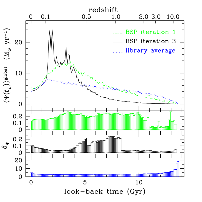
Figure 4: Top panel: resolved SFH of M51a, obtained with the BSP algorithm in age bins 100 Myr wide. Dashed-dotted green line: result obtained after BSP iteration number 1. Solid black line: result after BSP iteration number 3. Dotted blue line: the average of all SFHs in the SSAG-2017 library, multiplied by the present-day resolved stellar mass. Second from top panel: relative error, $\delta_{\Psi}=\frac{\sigma_{\Psi}}{\psi}$, for BSP iteration number 1. Third from top panel: relative error for BSP iteration number 3. Bottom panel: relative error for the average of SFHs in the SSAG-2017 library.

4.1 Radial gradients in SFHs

For each value of $t_{L}$ we have obtained a 2D map of the SFR (a total of 137 maps). In Figure 5 we show the present-day SFR-map for BSP iterations number 1 and 3, respectively. These SFR-maps were deprojected assuming an inclination angle of $20\degr$, and a position angle of $172\degr$ (Leroy et al., 2008). From these deprojected SFR-maps we then obtained the azimuthally averaged SFR $\langle\overline{\Psi(t_{L})}\rangle^{\rm azimuthal}$, for annuli at diverse radii ($R$). The results for all the radial profiles are displayed in Figure 6, where we present the outcome for BSP iterations 1 and 3, in the left and right panels, respectively. Both results show a decreasing SFR with radius. The same behaviour (see Figure 7) was obtained by González Delgado et al. (2016) with IFU data from the Calar Alto Legacy Integral Field Area survey (CALIFA, Sánchez et al., 2012). These results have also been corroborated by independent studies (see e.g., Pilkington et al., 2012; Nelson et al., 2016). In the case of M51a, we also find that the SFR activity is more localised at shorter radii and look-back times of $1<t_{L}<5$ Gyr, in BSP iteration number 3; conversely, the maximum-likelihood result (BSP iteration number 1) entails a wider spread in $t_{L}$.

Figure 5: Left: M51a SFR-map at $t_{L}=0$ derived with the BSP algorithm, iteration number 1. Right: same as left panel, for BSP iteration number 3. SFR in M_☉ Gyr^-1 pc^-2.

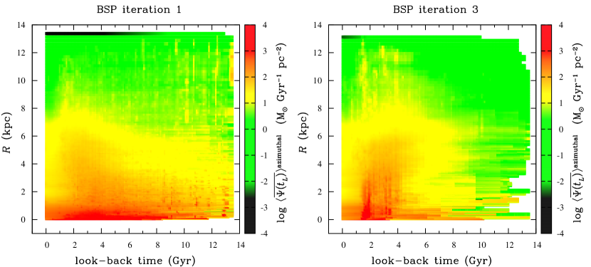
Figure 6: Azimuthally averaged SFR $\langle\overline{\Psi(t_{L})}\rangle^{\rm azimuthal}$ in (M_☉ Gyr^-1 pc^-2). Left: BSP iteration number 1. Right: BSP iteration number 3. The $y$-axis indicates the radius ($R$) measured from the centre of the object in kpc.

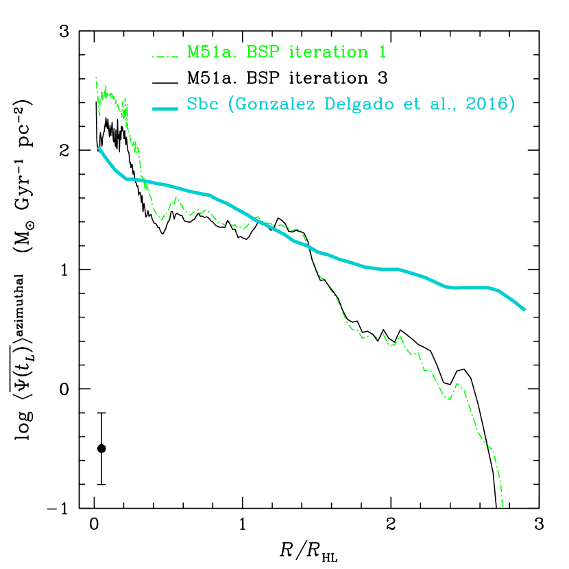
Figure 7: Azimuthally averaged SFR at $t_{L}=0$, in half-light radius, $R_{\rm HL}$, units. For M51a, the half-light radius is estimated from the SDSS $g$-band similarly to González Delgado et al. (2014), resulting in $R_{\rm HL}=4.7$ kpc. Dashed-dotted green line: M51a result obtained after BSP iteration number 1. Solid black line: M51a result after BSP iteration number 3. Solid turquoise thick line: González Delgado et al. (2016) average for Sbc galaxies.

5 Discussion

5.1 SFH parameterization

The recovery of the SFH of individual galaxies is essential to understand their evolution in the universe (e.g., Cid Fernandes et al., 2005; Ocvirk et al., 2006; Tojeiro et al., 2007, 2009; Weisz et al., 2014; Iyer & Gawiser, 2017; Williams et al., 2017). Commonly assumed simple forms of the SFH are a constant SFR ($\Psi$) with an abrupt cutoff at some time, and an exponentially declining function of time with a sharp rise at the beginning (e.g., Tinsley, 1972; Bruzual A., 1983). Recent studies have proposed functional forms that include a period of rising $\Psi$ (not necessarily sharp) at early times, followed by a peak of SF, and then a decline in $\Psi$ (not necessarily exponential) until the present-day value (e.g., Gladders et al., 2013; Pacifici et al., 2016). Gavazzi et al. (2002) suggested a ‘delayed-exponential’ or ‘à la Sandage’ SFH, with a delayed rise of $\Psi$ up to a maximum, followed by an exponential decrease. Maraston et al. (2010) propounded an exponentially increasing $\Psi$ to describe the early SFH of $z\sim 2$ galaxies. Behroozi et al. (2013) posited that the best-fit for various constraints on individual histories is a double power-law with four free parameters. Assuming that the SFH of individual galaxies follows a functional form similar to the cosmic star formation rate density (symmetric with logarithmic time, e.g., Madau et al., 1998), log-normal SFHs have also been suggested (e.g., Gladders et al., 2013; Dressler et al., 2016; Diemer et al., 2017).

As shown in Figure 4, for BSP iteration number 1 (maximum-likelihood estimate), $\langle\Psi(t_{L})\rangle^{\rm global}$ rises from the Big Bang until $\sim$ 4 Gyr ago, then stays fairly constant until about 2.5 Gyr ago when it starts to decline. For BSP iteration number 3 the SFH can be roughly characterised by three exponential time periods, as illustrated by Figure 8. For each of these periods we fit $\Psi(t)$ as

$$~{}\Psi(t)=A\exp\left(-\frac{t-t_{0}}{\tau}\right),$$ (6)

where $t_{0}$, $t$ are the beginning and ending times of the periods in time elapsed since the Big Bang, related to the look-back time by $t_{L}$(Gyr)$=13.721-t$, and $\tau$ is the characteristic $e$-folding time. The fitted parameters for each time period are given in Table 1. The first two time periods are adequately fitted with an exponentially increasing $\Psi(t)$, i.e., a negative $e$-folding time (or ‘inverted-$\tau$’ model, Maraston et al., 2010), whereas the last time period corresponds to $\Psi(t)$ declining exponentially until the present day. Superimposed on top of the most recent two exponential segments of $\Psi(t)$ we find three bursts of star formation at $t\approx$ 9.7, 10.4, and 11.9 Gyr after the Big Bang, or $t_{L}\approx$ 3.6, 3.3, and 1.8 Gyr, being the latter the most prominent. The SFH is not symmetric in logarithmic time.

Table 1: Fitted parameters of equation 6 for the time periods, $\Delta t$ (time since the Big Bang), shown in Figure 8.

$\Delta t$ (Gyr)	A (M☉ yr-1)	$t_{0}$ (Gyr)	$\tau$ (Gyr)
0.3 - 1.1	0.03	0.3	-0.703
1.1 - 10.1	0.08	1.1	-1.801
10.1 - 13.7	17.13	10.1	2.552

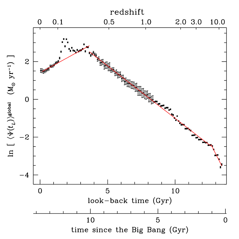
Figure 8: Fits (solid red lines, see Table 1) to the SFH of M51a after BSP iteration number 3 (black points). Error bars represent the absolute error in $\langle\Psi(t_{L})\rangle^{\rm global}$, propagated for the natural logarithm function ($\ln$).

In Figure 9 we show the mass $M(t)$ turned into stars until time $t$, estimated from

$$M(t)={\int_{0}^{t}\langle\Psi(t^{\prime})\rangle^{\rm global}{\rm d}t^{\prime}}.$$ (7)

The resulting $M(t)$ for BSP iteration number 3 has an overall shape that is qualitatively similar to the one obtained for Milky Way analogues (Diemer et al., 2017). The present-day resolved stellar mass of M51a is $M^{\rm BSP}_{*}=(3.98\pm 0.09)\times 10^{10}$ M_☉, which is marked by the long-dashed (horizontal) red line in Figure 9. The present-day value of $M(t)$ is $M_{\rm tot}=6.40\times 10^{10}$ M_☉, which indicates that $\sim 38$ per cent of this mass has been returned to the ISM, during the lifetime of the galaxy. The change from exponentially increasing $\Psi$ (negative $\tau$) to exponentially decreasing $\Psi$ (positive $\tau$), occurs at $t\sim 10.1$ Gyr after the Big Bang. Interestingly, $\sim 35$ per cent of the stellar mass is formed in the phase of negative $\tau$, and the remaining 65 per cent in the phase of positive $\tau$ (see Figure 9).

Figure 9: Mass processed in stars, $M(t)$ in M${}_{\sun}/10^{10}$, for M51a. Dashed-dotted green line: result after BSP iteration number 1. Solid black line: result after BSP iteration number 3. Long-dashed (horizontal) red line: present-day total resolved stellar mass obtained from the BSP algorithm (Martínez-García et al., 2017). Long-dashed-dotted (vertical) blue line: $t=10.1$ Gyr.

As a consistency check, we have used Bruzual & Charlot (2003) to build a galaxy model following the SFH depicted in Figure 8. At the present epoch this model reproduces quite well the integrated luminosity and colours of M51a, provided that we allow for a dust content as described by the Charlot & Fall (2000) prescription with $\tau_{V}\approx 1$. Although not a straightforward comparison, since spatially-unresolved results may differ significantly from resolved ones ($\sim 10-20$ per cent, Martínez-García et al., 2017), this optical depth is consistent with our BSP iteration number 3 results, namely, $\langle\tau_{V}\rangle=0.93$, and median $\tau_{V}=0.78$. If we ignore the negative $\tau$ segments of $\Psi(t)$ in Figure 8, we get a model that still resembles the observed galaxy at the present epoch. Both models are identical in the UV, but differ in flux in an amount that increases with spectral wavelength. The two models also differ in their dust content and age (because of their different onsets of SF). The model that omits the negative $\tau$, being fainter in the visible and NIR, will result in a higher estimate of the galaxy mass.

5.2 The recent SFH of M51a

The SFH of M51a has been the subject of various studies (e.g., Kaleida & Scowen, 2010; Kang et al., 2015). Salo & Laurikainen (2000) investigated two numerical models for the M51 interacting system. One of them predicts a single disc-plane crossing of the companion (M51b); the other anticipates several crossings. In both models, the companion’s disc-plane crossing responsible for the current spiral structure occurred 400-500 Myr ago. On the other hand, the multiple crossing model predicts another more recent disc-plane crossing about 50-100 Myr ago. From the observational point of view, the cluster formation rate in M51a also presents a large increase 50-70 Myr ago (Bastian et al., 2005; Gieles et al., 2005). In Figure 10 we present the most recent 2 Gyr of the SFH obtained with the BSP algorithm in age bins of 10 Myr (10 times narrower than in Figure 4). We have indicated the time periods of 50-100, and 400-500 Myr ago with shaded regions. Our results (BSP iteration number 3) indicate an increase of $\sim 29$ per cent in $\langle\Psi(t_{L})\rangle^{\rm global}$ 50-100 Myr ago, compared to the present-day value, $\langle\Psi(t_{L})\rangle^{\rm global}=3.9\pm 0.4$ M_☉ yr^-1. However, we find no SF burst 400-500 Myr ago.

Also, in Figure 10 (red point) we show the present-day attenuation-corrected (for extinction internal to the galaxy itself) $\Psi_{{\rm H}\alpha}$, derived from the combination of H$\alpha$ and $24\micron$ luminosities. We adopt the Kennicutt (1998) and Kennicutt et al. (2009, their equation 12) calibrations, along with the Kennicutt et al. (2008) H$\alpha$ + [N ii], and Dale et al. (2007) $24\micron$ integrated fluxes. We correct for our adopted distance and Galactic reddening, and for [N ii] emission (Kennicutt et al., 2008). We divide the resulting $\Psi_{{\rm H}\alpha}$ by $1.7\pm 0.3$ to convert to a Chabrier (2003) IMF, since Kennicutt (1998) calibrations correspond to a Salpeter (1955) IMF. We estimate a value of $\Psi_{{\rm H}\alpha}=1.34\pm 0.32$ $M_{\sun}$ yr^-1. Our previously derived $\langle\Psi(t_{L})\rangle^{\rm global}$ is $\sim 3$ times bigger than $\Psi_{{\rm H}\alpha}$. The measurements are different by $3.55\sigma$.

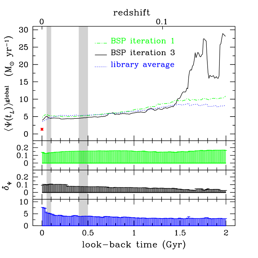
Figure 10: The recent 2 Gyr SFH of M51a, obtained with the BSP algorithm in age bins of 10 Myr. Same nomenclature as in Figure 4. Shaded regions in gray indicate time periods of 50-100 and 400-500 Myr ago. Red point: the attenuation-corrected $\Psi_{{\rm H}\alpha}$ obtained from H$\alpha$ and $24\micron$ luminosities (Kennicutt, 1998; Kennicutt et al., 2009).

6 A different choice of prior PDF

Up to this point we have applied the Martínez-García et al. (2017) BSP algorithm to infer the SFH of M51a. This is done by assuming a prior PDF for $\Upsilon^{K_{s}}_{*}$ in equation 1. In this section we explore the use of prior PDFs for other parameters, for instance, the stellar metallicity, $Z$, the dust content characterised by $\tau_{V}$, and the stellar age characterised by T_form. For this purpose, equation 1 takes the form

$$~{}P(\mathbf{X}\mid C)\propto\exp\left(-\frac{\chi^{2}}{2}\right)\exp\left(-\frac{1}{2}\left[\frac{\mathbf{X}^{\rm prior}-\mathbf{X}}{\sigma_{\mathbf{X}}}\right]^{2}\right),$$ (8)

where $\mathbf{X}$ is replaced by $Z$, $\tau_{V}$, or T_form, and $\sigma_{\mathbf{X}}\approx\sigma_{\rm mag}\mathbf{X}^{\rm prior}$. We apply BSP in a similar manner to that used with the $\Upsilon^{K_{s}}_{*}$ prior PDF. The only difference is when moving from iteration number 2 to iteration number 3: we compute the required interpolated structure directly from the ‘backbone’ $\mathbf{X}$ pixels, instead of interpolating it from the ‘backbone’ mass pixels (cf. Martínez-García et al., 2017). The results of this exercise are shown in Figure 11. The SFH curves for $Z$ and $\tau_{V}$ follow an almost identical behaviour to the one obtained from the maximum-likelihood estimate (BSP iteration number 1). Contrariwise, the T_form SFH curve presents a shape very similar to our SFH templates (see Figure 3), with T${}_{\rm form}\sim 5.5$ Gyr. This result is not surprising, since the median T_form value of the whole disk, after BSP iteration number 1, is T${}_{\rm form}=5.71$ Gyr. In this manner, we are basically recovering the prior SFH we assumed before. A difference between the results obtained with the $\Upsilon^{K_{s}}_{*}$ and the T_form priors, respectively, is that the latter still produces mass-maps with a filamentary structure. We have corroborated this effect qualitatively by visual inspection, and quantitatively by calculating the normalised Pearson correlation coefficient between two mass-maps,

$$~{}r=\frac{\sum\limits_{j}\sum\limits_{i}(F_{ij}-\bar{F})(G_{ij}-\bar{G})}{\sqrt{\sum\limits_{j}\sum\limits_{i}(F_{ij}-\bar{F})^{2}}\sqrt{\sum\limits_{j}\sum\limits_{i}(G_{ij}-\bar{G})^{2}}},$$ (9)

where $F_{ij}$ is the stellar mass surface density, $\rho_{*}$, of the $i^{\rm th},j^{\rm th}$ pixel in the first mass-map, $G_{ij}$ is the $\rho_{*}$ of the $i^{\rm th},j^{\rm th}$ pixel in the second mass-map, $\bar{F}$ is the mean $\rho_{*}$ of the first mass-map, and $\bar{G}$ is the mean $\rho_{*}$ of the second mass-map. We estimate $r$ between the resulting mass-maps for BSP iterations number 1 and 3, adopting the $\Upsilon^{K_{s}}_{*}$, $Z$, $\tau_{V}$, and T_form priors. The uncertainties in $r$ are estimated via bootstrap methods (e.g., Bhavsar, 1990). The results are plotted in Figure 12, where a value of $r=1$ would indicate a perfect match between the spatial structure of both mass-maps. As expected, the $r$ value for the $\Upsilon^{K_{s}}_{*}$ prior PDF indicates a greater discrepancy between the mass-maps when compared to the $r$ values obtained when adopting the $Z$, $\tau_{V}$, or T_form prior PDFs. As stressed out by Martínez-García et al. (2017), an advantage of using a spatial structure prior, by means of a $\Upsilon^{\rm NIR}_{*}$ prior, with our BSP algorithm, is its independence from SPS model parameters, e.g., SFH, metallicity, dust, age, etc.

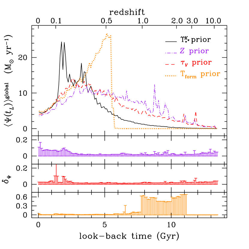
Figure 11: Top panel: same as Figure 4 for different prior PDFs. All SFH curves correspond to results after BSP iteration number 3. Solid black, dashed-dotted purple, dashed red, and dotted orange lines: mass-to-light ratio ($\Upsilon^{K_{s}}_{*}$), stellar metallicity ($Z$), dust ($\tau_{V}$), and stellar age (T_form) priors, respectively. Second, third, and fourth from top panels: relative errors, $\delta_{\Psi}=\frac{\sigma_{\Psi}}{\psi}$, for the $Z$, $\tau_{V}$, and T_form priors, respectively.

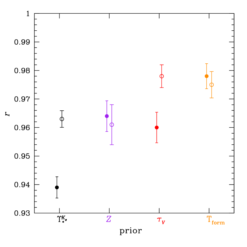
Figure 12: Solid symbols: Pearson correlation coefficient, $r$ (see equation 9), between the mass-maps resulting from BSP iterations number 1 and 3. The adopted prior PDF is indicated on the $x$-axis for the mass-to-light ratio $\Upsilon^{K_{s}}_{*}$, the metallicity $Z$, the dust content $\tau_{V}$, and the stellar age T_form, respectively. Open symbols: a radially varying prior PDF is assumed for BSP iteration number 2 (see section 6.1).

6.1 A radially varying prior PDF

As described in section 3, the second BSP iteration assumes a constant stellar mass-to-light ratio $\Upsilon_{*}$, in the NIR, for the entire disk, i.e., a constant $\Upsilon_{*}^{\rm prior}$, or a constant $\mathbf{X}$ parameter, in equations 1 or 8, respectively. In this section we explore the use of a radially varying $\mathbf{X}$. For this purpose we use the $\mathbf{X}$ radial profiles resulting from BSP iteration number 1. However, we must remember that the mass-map generated from this maximum-likelihood fit has a bias in its spatial structure. The radial profiles for $\Upsilon^{K_{s}}_{*}$, $Z$, $\tau_{V}$, and T_form are shown in Figure 13. We use these radial profiles to generate a surface of revolution for each $\mathbf{X}$ parameter. We synthesise some images from these surfaces, project them to mimic the disk orientation, and use them in BSP iteration number 2, instead of the constant plane previously assumed. The resulting SFHs of this test are shown in Figure 14. We find a tendency to follow the curve for BSP iteration number 1 in all the parameters, which is more accentuated for the $Z$ and $\tau_{V}$ curves. The Pearson correlation coefficient, $r$ (see Figure 12, open symbols), between the mass-maps of BSP iterations number 1 and 3 indicate that these assumptions do not improve the mass-maps more than assuming a constant $\Upsilon^{K_{s}}_{*}$ for BSP iteration number 2.

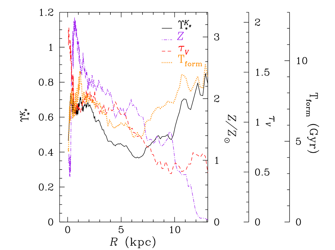
Figure 13: Azimuthally averaged $\mathbf{X}$ parameters vs. radius, $R$ (kpc), for M51a deprojected maps, after BSP iteration number 1. Solid black line: mass-to-light ratio ($\Upsilon^{K_{s}}_{*}$). Dashed-dotted purple line: stellar metallicity $Z/Z_{\sun}$. Dashed red line: dust ($\tau_{V}$). Dotted orange line: stellar age (T_form).

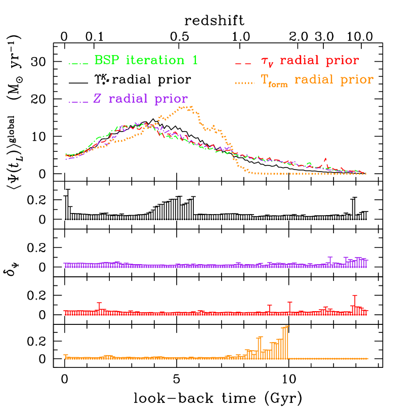
Figure 14: Resulting SFHs of M51a after a radially varying prior PDF (see section 6.1). Dashed-dotted green line: result after BSP iteration number 1. Solid black, dashed-dotted purple, dashed red, and dotted orange lines indicate the SFH after BSP iteration number 3, assuming a radially varying $\Upsilon^{K_{s}}_{*}$, $Z$, $\tau_{V}$, and T_form prior in BSP iteration number 2, respectively. Second, third, fourth, and fifth from top panels: relative errors for the $\Upsilon^{K_{s}}_{*}$, $Z$, $\tau_{V}$, and T_form SFHs, respectively.

7 Conclusions

We have introduced a novel technique to determine the SFH of a galaxy. The method is based on spectral fitting pixel by pixel the resolved image of the galaxy in various photometric bands (UV to NIR), using our BSP algorithm (Martínez-García et al., 2017). We obtain the SFH for each pixel in the galaxy, i.e., the SFH-map of the galaxy, an image of the galaxy resolved in space and time. We can thus characterise the underlying shape of the SFH from the Big Bang to the present day, together with individual episodes, or bursts, of star formation. We have applied this technique to M51a and find that its global SFH consists of an exponentially increasing SFR $\Psi(t)$ lasting until $\approx$ 10 Gyr after the Big Bang, followed by an exponentially decreasing $\Psi(t)$ until the present day, with a main burst of star formation superimposed during the declining phase. These results show that, while the SFH of each individual pixel of a galaxy can be adequately fitted by an exponentially decaying $\Psi(t)$, the global SFH of the galaxy may behave differently in time. Nevertheless, we recognise that as in every problem solved with Bayesian statistics, the solution will reflect the physical properties of the prior used (SSAG), and we do not rule out that a radical change in the SSAG properties, may result in a drastic change for the SFH of M51a. The SFH of a disk galaxy has to be compatible with the present-day stellar mass distribution as inferred from NIR images. This is only achieved when a mass-to-light ratio prior PDF is adopted in BSP. When applied to a larger sample of galaxies this method can help us constrain current models of galaxy evolution, as well as the cosmic SFH (e.g., Heavens et al., 2004; Madau & Dickinson, 2014).

Appendix A The implicit SFHs prior

In this appendix we discuss the implicit prior placed on the SFHs by the adopted SSAG-2017 library. The average of all SFHs, $\langle\Psi(t_{L})\rangle^{\rm library~{}average}$ (dotted blue line in Figure 4), is dominated by the PDF of the T_form parameter, which has a roughly uniform distribution between 1.5 and 13.7 Gyr (see Figure 15, blue line histogram). The T_form PDF is correlated to the form of the $\langle\Psi(t_{L})\rangle^{\rm library~{}average}$ curve in the following manner. At look-back times $t_{L}\sim$13.7 Gyr only a few templates contribute to $\langle\Psi(t_{L})\rangle^{\rm library~{}average}$. At look-back times $t_{L}\lesssim$13.7 Gyr the $\langle\Psi(t_{L})\rangle^{\rm library~{}average}$ has contributions from the accumulated $\langle\Psi(t_{L})\rangle$ for $t_{L}\sim$13.7 Gyr, and the corresponding $\langle\Psi(t_{L})\rangle$ for $t_{L}\lesssim$13.7 Gyr. This has the consequence of increasing $\langle\Psi(t_{L})\rangle^{\rm library~{}average}$ as $t_{L}$ decreases within the interval $1.5\lesssim t_{L}\lesssim 13.7$ Gyr. At $t_{L}\lesssim 1.5$ Gyr, $\langle\Psi(t_{L})\rangle^{\rm library~{}average}$ decreases together with $t_{L}$, as a consequence of the T_form PDF.

We select from the SSAG-2017 library the subset shown by the dark red histogram in Figure 15. This T_form PDF was chosen because it is radically different from the original SSAG-2017 library (blue histogram). The resulting library consists of $\sim 3.5\times 10^{4}$ templates. With this subset-I library, we apply BSP in an identical manner as before. The results are shown in Figure 16. In the same figure we also plot our SSAG-2017 (Figure 4) results with thinner lines. In order to verify the equality (or not) between both results we perform a Kolmogorov-Smirnov (KS) test. The KS test compares the cumulative empirical distribution function of some sample data with the expected distribution (or expected SFH curve in our case). The KS statistic, $D$, is used to compute the probability $p_{\rm value}$, which gauges the evidence against dissimilar distributions. Typically, when $p_{\rm value}>0.05$, there is not enough evidence to conclude that the two distributions differ from each other, whereas $p_{\rm value}<0.05$ indicates distinct distributions. In Table 2 we show the results of the KS test between the full SSAG-2017 and the subset-I libraries. For the BSP curves, the $p_{\rm value}$ probabilities indicate analogous distributions, while for the library average curves, the $p_{\rm value}$ point to different distributions, thus demonstrating no correlation between our implicit SFHs prior and BSP results.

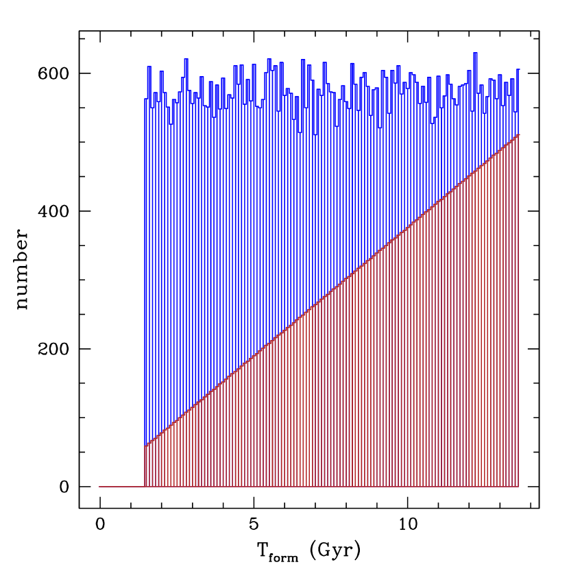
Figure 15: T_form histograms for the full SSAG-2017 library (blue) and the subset-I library (dark red).

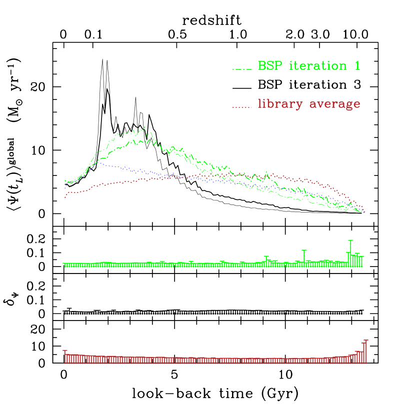
Figure 16: Same as Figure 4 for the T_form PDF shown by the dark red histogram in Figure 15. Dotted dark red line: the average of all SFHs in the subset-I library, multiplied by the present-day resolved stellar mass. For comparison purposes, the thinner lines show the same curves plotted in Figure 4.

Table 2: KS test results between SSAG-2017 and other libraries.

Library	SFH curve	$p_{\rm value}$	Figure
subset-I	BSP-1	0.1379	16
	BSP-3	0.1379
	library average	0.0043
subset-II	BSP-1	0.0763	17
(no bursts)	BSP-3	0.0469
	library average	0.0018
subset-III	BSP-1	0.0762	18
(bursts only)	BSP-3	0.3752
	library average	0.0001
SSAG-2015	BSP-1	0.0010	19
	BSP-3	0.2348
	library average	0.5586
subset-IV	BSP-1	0.0281	20
	BSP-3	0.3752
	library average	1.0000

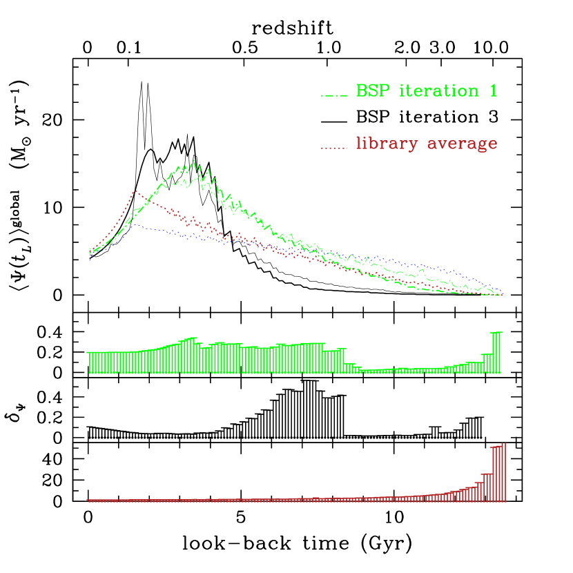
Figure 17: Same as Figure 4 for the subset-II (no bursts) library. Dotted dark red line: the average of all SFHs in the subset-II library, multiplied by the present-day resolved stellar mass. For comparison purposes, the thinner lines show the same curves plotted in Figure 4.

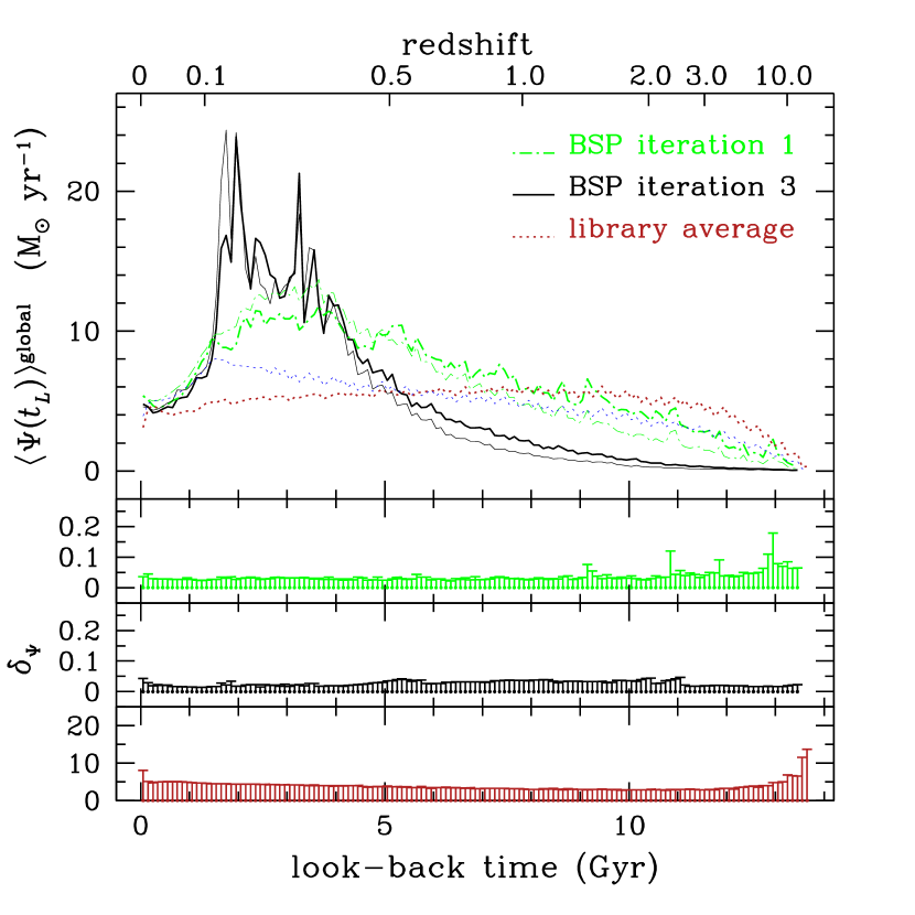
Figure 18: Same as Figure 4 for the subset-III (bursts only) library. Dotted dark red line: the average of all SFHs in the subset-III library, multiplied by the present-day resolved stellar mass. The thinner lines show the same curves plotted in Figure 4.

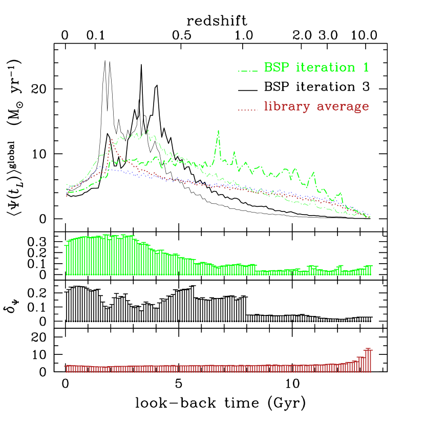
Figure 19: Same as Figure 4 for the SSAG-2015 library. Dotted dark red line: the average of all SFHs in the SSAG-2015 library, multiplied by the present-day resolved stellar mass. The thinnest lines show the same curves plotted in Figure 4.

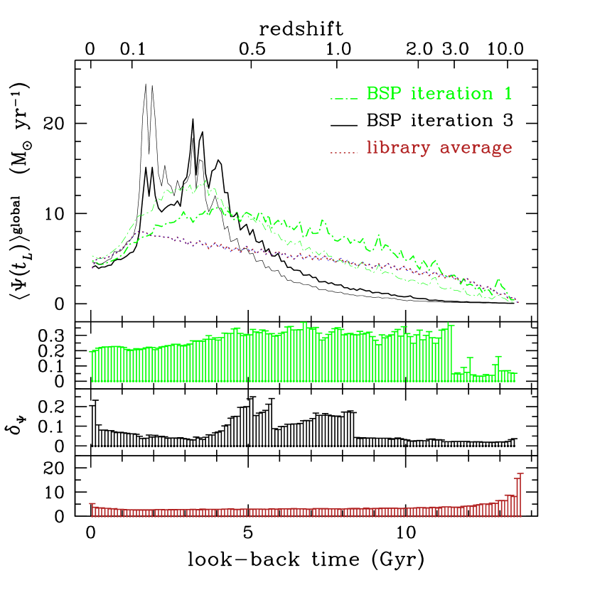
Figure 20: Same as Figure 4 for the subset-IV library. Dotted dark red line: the average of all SFHs in the subset-IV library, multiplied by the present-day resolved stellar mass. The thinnest lines show the same curves plotted in Figure 4.

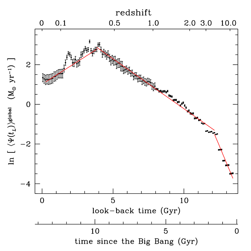
Figure 21: Same as Figure 8 for the SSAG-2015 library (see also Table 3.)

Table 3: Fitted parameters of equation 6 for the time periods, $\Delta t$ (time since the Big Bang), shown in Figure 21.

$\Delta t$ (Gyr)	A (M☉ yr-1)	$t_{0}$ (Gyr)	$\tau$ (Gyr)
0.3 - 1.6	0.02	0.3	-0.583
1.6 - 9.9	0.27	1.6	-1.984
9.9 - 13.5	16.00	9.9	2.190

We also compare the results obtained with other three different libraries. The first one consists in a subset (II) of the SSAG-2017 library, of all the templates with no superimposed burst of SF. The second one (subset-III) includes only the SSAG-2017 templates with a superimposed burst of SF. Additionally, we use the 2015 version of the SSAG as another comparison case. The SFH curves are shown in Figures 17, 18, and 19, for the subset-II, subset-III, and SSAG-2015 libraries, respectively. In Table 2 we show the KS test results for each case. As expected, the no-bursts library (subset II) reproduces the general shape of the SFH curve without the bursts peaks. For the only-bursts library (subset III), the SFH curves are nearly identical to the SSAG-2017 library case. For the SSAG-2015 results, the BSP iteration number 1 curve differs from the SSAG-2017 result, while the BSP iteration number 3 curves reveal similar features but different $\langle\Psi(t_{L})\rangle^{\rm global}$ amplitudes for both libraries. This behaviour is mainly due to the different metallicity ranges, since for SSAG-2015, $Z/Z_{\sun}$ is distributed almost uniformly between 0.02 and 2.5. To corroborate this effect we separate another subset (IV) of the SSAG-2017, consisting of all the templates where $0.02\leqq Z/Z_{\sun}\leqq 2.5$. The results are shown in Figure 20, where we can appreciate a very similar outcome as in Figure 19 (see also Table 2). By comparing the SSAG-2015 and the subset-IV SFH curves, for BSP iteration number 3, we obtain $p_{\rm value}=0.9251$. In this manner, a narrower metallicity range can affect the amplitudes of the SFH curves for certain segments, but the qualitative behaviour would remain the same.

Finally, in Figure 21 (solid red lines) and Table 3, we show the fits to the SFH of M51a after BSP iteration number 3, adopting the SSAG-2015 library. For this case, the turnover from exponentially increasing $\Psi$ (negative $\tau$) to exponentially decreasing $\Psi$ (positive $\tau$) occurs at $t\sim 9.9$ Gyr. A very similar value is obtained from the fits shown in Figure 8, where $t\sim 10.1$ Gyr. In conclusion, the implicit prior PDF of the SFH, determined by the adopted SPS library, has no relevant effects on the results.

References

- Abdurro’uf (2017) Abdurro’uf, A., Masayuki 2017, MNRAS, 469, 2806
- Alam et al. (2015) Alam, S., Albareti, F. D., Allende Prieto, C., et al. 2015, ApJS, 219, 12
- Aniano et al. (2011) Aniano, G., Draine, B. T., Gordon, K. D., & Sandstrom, K. 2011, PASP, 123, 1218
- Bastian et al. (2005) Bastian, N., Gieles, M., Lamers, H. J. G. L. M., Scheepmaker, R. A., & de Grijs, R. 2005, A&A, 431, 905
- Behroozi et al. (2013) Behroozi, P. S., Wechsler, R. H., & Conroy, C. 2013, ApJ, 770, 57
- Bennett et al. (2014) Bennett, C. L., Larson, D., Weiland, J. L., & Hinshaw, G. 2014, ApJ, 794, 135
- Bhavsar (1990) Bhavsar, S. P. 1990, Errors, Bias and Uncertainties in Astronomy, 107
- Bruzual A. (1983) Bruzual A., G. 1983, ApJ, 273, 105
- Bruzual & Charlot (2003) Bruzual, G., & Charlot, S. 2003, MNRAS, 344, 1000
- Cano-Díaz et al. (2016) Cano-Díaz, M., Sánchez, S. F., Zibetti, S., et al. 2016, ApJ, 821, L26
- Chabrier (2003) Chabrier, G. 2003, PASP, 115, 763
- Charlot & Fall (2000) Charlot, S., & Fall, S. M. 2000, ApJ, 539, 718
- Chen et al. (2012) Chen, Y.-M., Kauffmann, G., Tremonti, C. A., et al. 2012, MNRAS, 421, 314
- Cid Fernandes et al. (2005) Cid Fernandes, R., Mateus, A., Sodré, L., Stasińska, G., & Gomes, J. M. 2005, MNRAS, 358, 363
- Dale et al. (2007) Dale, D. A., Gil de Paz, A., Gordon, K. D., et al. 2007, ApJ, 655, 863
- de Amorim et al. (2017) de Amorim, A. L., García-Benito, R., Cid Fernandes, R., et al. 2017, MNRAS, 471, 3727
- de Vaucouleurs et al. (1991) de Vaucouleurs, G., de Vaucouleurs, A., Corwin, H. G., Jr., et al. 1991, Third Reference Catalogue of Bright Galaxies (RC3)
- Díaz-García et al. (2015) Díaz-García, L. A., Cenarro, A. J., López-Sanjuan, C., et al. 2015, A&A, 582, A14
- Diemer et al. (2017) Diemer, B., Sparre, M., Abramson, L. E., & Torrey, P. 2017, ApJ, 839, 26
- Dressler et al. (2016) Dressler, A., Kelson, D. D., Abramson, L. E., et al. 2016, ApJ, 833, 251
- Ibarra-Medel et al. (2016) Ibarra-Medel, H. J., Sánchez, S. F., Avila-Reese, V., et al. 2016, MNRAS, 463, 2799
- Iyer & Gawiser (2017) Iyer, K., & Gawiser, E. 2017, ApJ, 838, 127
- Gavazzi et al. (2002) Gavazzi, G., Bonfanti, C., Sanvito, G., Boselli, A., & Scodeggio, M. 2002, ApJ, 576, 135
- Gieles et al. (2005) Gieles, M., Bastian, N., Lamers, H. J. G. L. M., & Mout, J. N. 2005, A&A, 441, 949
- Gil de Paz et al. (2007) Gil de Paz, A., Boissier, S., Madore, B. F., et al. 2007, ApJS, 173, 185
- Gladders et al. (2013) Gladders, M. D., Oemler, A., Dressler, A., et al. 2013, ApJ, 770, 64
- Gonzalez & Graham (1996) Gonzalez, R. A., & Graham, J. R. 1996, ApJ, 460, 651
- González Delgado et al. (2014) González Delgado, R. M., Pérez, E., Cid Fernandes, R., et al. 2014, A&A, 562, A47
- González Delgado et al. (2015) González Delgado, R. M., García-Benito, R., Pérez, E., et al. 2015, A&A, 581, A103
- González Delgado et al. (2016) González Delgado, R. M., Cid Fernandes, R., Pérez, E., et al. 2016, A&A, 590, A44
- Heavens et al. (2004) Heavens, A., Panter, B., Jimenez, R., & Dunlop, J. 2004, Nature, 428, 625
- Kaleida & Scowen (2010) Kaleida, C., & Scowen, P. A. 2010, AJ, 140, 379
- Kang et al. (2015) Kang, X., Chang, R., Zhang, F., Cheng, L., & Wang, L. 2015, MNRAS, 449, 414
- Kennicutt (1998) Kennicutt, R. C., Jr. 1998, ARA&A, 36, 189
- Kennicutt et al. (2008) Kennicutt, R. C., Jr., Lee, J. C., Funes, J. G., et al. 2008, ApJS, 178, 247-279
- Kennicutt et al. (2009) Kennicutt, R. C., Jr., Hao, C.-N., Calzetti, D., et al. 2009, ApJ, 703, 1672-1695
- Leroy et al. (2008) Leroy, A. K., Walter, F., Brinks, E., et al. 2008, AJ, 136, 2782
- Madau et al. (1998) Madau, P., Pozzetti, L., & Dickinson, M. 1998, ApJ, 498, 106
- Madau & Dickinson (2014) Madau, P., & Dickinson, M. 2014, ARA&A, 52, 415
- Magris et al. (2015) Magris C., G., Mateu P., J., Mateu, C., et al. 2015, PASP, 127, 16
- Maraston et al. (2010) Maraston, C., Pforr, J., Renzini, A., et al. 2010, MNRAS, 407, 830
- Martínez-García et al. (2017) Martínez-García, E. E., González-Lópezlira, R. A., Magris C., G., & Bruzual A., G. 2017, ApJ, 835, 93
- Mentuch Cooper et al. (2012) Mentuch Cooper, E., Wilson, C. D., Foyle, K., et al. 2012, ApJ, 755, 165
- McQuinn et al. (2016) McQuinn, K. B. W., Skillman, E. D., Dolphin, A. E., Berg, D., & Kennicutt, R. 2016, ApJ, 826, 21
- Nelson et al. (2016) Nelson, E. J., van Dokkum, P. G., Förster Schreiber, N. M., et al. 2016, ApJ, 828, 27
- Ocvirk et al. (2006) Ocvirk, P., Pichon, C., Lançon, A., & Thiébaut, E. 2006, MNRAS, 365, 46
- Pacifici et al. (2016) Pacifici, C., Kassin, S. A., Weiner, B. J., et al. 2016, ApJ, 832, 79
- Peek & Schiminovich (2013) Peek, J. E. G., & Schiminovich, D. 2013, ApJ, 771, 68
- Pilkington et al. (2012) Pilkington, K., Few, C. G., Gibson, B. K., et al. 2012, A&A, 540, A56
- Rosa-González et al. (2002) Rosa-González, D., Terlevich, E., & Terlevich, R. 2002, MNRAS, 332, 283
- Rix & Rieke (1993) Rix, H.-W., & Rieke, M. J. 1993, ApJ, 418, 123
- Salim et al. (2007) Salim, S., Rich, R. M., Charlot, S., et al. 2007, ApJS, 173, 267
- Salim et al. (2016) Salim, S., Lee, J. C., Janowiecki, S., et al. 2016, ApJS, 227, 2
- Salo & Laurikainen (2000) Salo, H., & Laurikainen, E. 2000, MNRAS, 319, 377
- Salpeter (1955) Salpeter, E. E. 1955, ApJ, 121, 161
- Sánchez et al. (2012) Sánchez, S. F., Kennicutt, R. C., Gil de Paz, A., et al. 2012, A&A, 538, A8
- Schlafly & Finkbeiner (2011) Schlafly, E. F., & Finkbeiner, D. P. 2011, ApJ, 737, 103
- Schlegel et al. (1998) Schlegel, D. J., Finkbeiner, D. P., & Davis, M. 1998, ApJ, 500, 525
- Sorba & Sawicki (2015) Sorba, R., & Sawicki, M. 2015, MNRAS, 452, 235
- Skrutskie et al. (2006) Skrutskie, M. F., Cutri, R. M., Stiening, R., et al. 2006, AJ, 131, 1163
- Tikhonov et al. (2009) Tikhonov, N. A., Galazutdinova, O. A., & Tikhonov, E. N. 2009, Astronomy Letters, 35, 599
- Tojeiro et al. (2007) Tojeiro, R., Heavens, A. F., Jimenez, R., & Panter, B. 2007, MNRAS, 381, 1252
- Tojeiro et al. (2009) Tojeiro, R., Wilkins, S., Heavens, A. F., Panter, B., & Jimenez, R. 2009, ApJS, 185, 1
- Tinsley (1972) Tinsley, B. M. 1972, A&A, 20, 383
- Weisz et al. (2014) Weisz, D. R., Dolphin, A. E., Skillman, E. D., et al. 2014, ApJ, 789, 147
- Williams et al. (2017) Williams, B. F., Dolphin, A. E., Dalcanton, J. J., et al. 2017, ApJ, 846, 145
- Wright (2006) Wright, E. L. 2006, PASP, 118, 1711
- Zibetti (2009) Zibetti, S. 2009, arXiv:0911.4956
- Zibetti, Charlot, & Rix (2009) Zibetti, S., Charlot, S., & Rix, H.-W. 2009, MNRAS, 400, 1181