Extended investigation of the twelve-flavor $\beta$-function

Abstract

We report new results from high precision analysis of an important BSM gauge theory with twelve massless fermion flavors in the fundamental representation of the SU(3) color gauge group. The range of the renormalized gauge coupling is extended from our earlier work [1] to probe the existence of an infrared fixed point (IRFP) in the $\beta$-function reported at two different locations, originally in [2] and at a new location in [3]. We find no evidence for the IRFP of the $\beta$-function in the extended range of the renormalized gauge coupling, in disagreement with [2, 3]. New arguments to guard the existence of the IRFP remain unconvincing [4], including recent claims of an IRFP with ten massless fermion flavors [5, 6] which we also rule out. Predictions of the recently completed 5-loop QCD $\beta$-function for general flavor number are discussed in this context.

1 History of the IRFP with 12 massless fermions

A conformal infrared fixed point (IRFP) of the $\beta$-function was reported earlier with critical gauge coupling $g_{*}^{2}\approx 6.2$ and interpreted as conformal behavior of the much studied BSM gauge theory with twelve massless fermions in the fundamental representation of the SU(3) color gauge group [2]. This result was claimed to confirm the original finding of the IRFP in [7, 8]. In disagreement with [2, 7, 8], the IRFP was refuted in [1]. Recently, responding to the negative findings in [1], the authors of [2] moved the IRFP to a revised new location $g_{*}^{2}\approx 7$ in [3].

The relocation of the IRFP followed the announcement of a new IRFP with ten massless fermion flavors in the fundamental representation of the SU(3) color gauge group [5, 6]. The claim in [5, 6] would imply that the theory with twelve flavors must also be conformal and the lower edge of the conformal window (CW) of multi-flavor BSM theories with fermions in the fundamental representation would be located below ten flavors. No trace of the reported IRFP with ten flavors was found from high precision simulations in large volumes [9]. Some related predictions of the recently completed 5-loop QCD $\beta$-function for general flavor number will be also discussed in this context.

Results are reported for the $\beta$-function from the analysis of high precision simulations in large volumes for $n_{f}=12$ flavors in two different renormalization schemes and two different implementations of the gauge field gradient flow on the lattice, providing convincing evidence for the non-existence of the IRFP in [3]. A preview from our forthcoming new publication on the $n_{f}=10$ $\beta$-function [9] is also added showing evidence for the non-existence of the IRFP published in this theory [5, 6].

2 Scale-dependent $\beta$-function on the lattice

The gradient flow based diffusion of the gauge fields on lattice configurations from Hybrid Monte Carlo (HMC) simulations became the method of choice for studying renormalization effects with great accuracy  [10, 11, 12, 13, 14]. In particular, we introduced earlier the gradient flow based scale-dependent renormalized gauge coupling $g^{2}(L)$ where the scale is set by the linear size $L$ of the finite volume [15]. This implementation is based on the gauge invariant trace of the non-Abelian quadratic field strength, $E(t)=-\frac{1}{2}{\rm Tr}F_{\mu\nu}F_{\mu\nu}(t)$, renormalized as a composite operator at gradient flow time $t$ on the gauge configurations and measured from the discretized lattice implementation, as in [11].

Following [15], we define the one-parameter family of renormalized non-perturbative gauge couplings where the volume-dependent gradient flow time $t(L)$ is set by a fixed value of $c=\sqrt{8t}/L$ from the one-parameter family of renormalization schemes. The renormalized gauge coupling $g^{2}(L)$ is directly determined from $E(t)=-\frac{1}{2}{\rm Tr}F_{\mu\nu}F_{\mu\nu}(t)$ on the gradient flow of the gauge field at a fixed value of $c$ which defines the renormalization scheme. The renormalization schemes $c=0.20$ and $c=0.25$ used in our work are identical to what was used in [2, 3] including periodic boundary conditions on gauge fields and anti-periodic boundary conditions on fermion fields in all four directions of the lattice.

A general method for the scale-dependent renormalized gauge coupling $g^{2}(L)$ was introduced earlier to probe the step $\beta$-function, defined as $(g^{2}(sL)-g^{2}(L))/\log(s^{2})$ for some preset finite scale change $s$ in the linear physical size $L$ of the four-dimensional volume in the continuum limit of lattice discretization [16]. In our adaptation of the step $\beta$-function staggered lattice fermions are used with stout smearing in the fermion Dirac operator. The implementation of the HMC evolution code is described in [1] together with further details on the lattice step function and its continuum limit. Identical procedures are followed here.

3 High precision twelve-flavor analysis in large volumes

In the continuum limit, the monotonic function $g^{2}(L)$ implies in any of the volume-dependent schemes that a selected value of the renormalized gauge coupling sets the physical size $L$ measured in some particular dimensionful physical unit. Fixed physical size $L$ on the lattice is equivalent to holding $g^{2}(L)$ fixed at some selected value as the lattice spacing $a$ is varied and the fixed physical length $L$ is held constant by the variation of the dimensionless linear scale $L/a$ as the bare lattice coupling is tuned without changing the selected fixed value of the renormalized gauge coupling. The continuum limit of the $\beta$-function at fixed $g^{2}(L)$ is obtained by $a^{2}/L^{2}\to 0$ extrapolation of the residual cut-off dependence detected as powers of $a^{2}/L^{2}$ in the step $\beta$-function at finite bare gauge couplings $g_{0}^{2}$ while the renormalized gauge coupling is held fixed.

In the convention we use, asymptotic freedom in the UV regime corresponds to a positive step $\beta$-function given by the perturbative loop expansion for small values of the renormalized coupling. In the infinitesimal derivative limit $s\!\to\!1$ the step $\beta$-function turns into the conventional one. It turns out that even at a step size as large as $s=2$ the step $\beta$-function tracks the conventional continuum $\beta$-function with very good accuracy and we use step $s=2$ throughout the analysis. If the conventional $\beta$-function of the theory possesses a conformal fixed point, the step $\beta$-function will have a zero at the critical gauge coupling $g_{*}^{2}$, independent of the scale $L$. Since the renormalized gauge coupling $g^{2}(L)$ is a monotonic function of $L$, the IRFP coupling $g_{*}^{2}$ is reached in the $L\to\infty$ limit.

3.1 SSC gradient flow with c=0.20 renormalization scheme

Precision tuning of the bare gauge coupling $6/g^{2}_{0}$ was used exclusively for each step calculation in [1] using the $c=0.20$ renormalization scheme with $s=2$ step size. The gauge field gradient flow was driven by the same tree-level improved Symanzik gauge action which generated the gauge configurations. The lattice implementation of the gauge field operator $E(t)=-\frac{1}{2}{\rm Tr}F_{\mu\nu}F_{\mu\nu}(t)$ used the clover construction which is known to reduce cut-off effects in the gradient flow [11]. SSC designates the setup with Symanzik gauge action driving both the gauge field gradient flow and the HMC evolution code, together with the clover operator implementation of $E(t)$. The three target groups A, B, C of the precision tuned run sets tested the IRFP with negative conclusions, in disagreement with what was reported in [2]. In this work we target the step $\beta$-function in an extended range of the renormalized gauge coupling to cover the interval where the relocated IRFP was recently reported [3]. For consistency check, we added to the analysis the WSC scheme in section 3.2 where the Symanzik action is replaced by the simple Wilson plaquette action to drive the gradient flow on the gauge configurations. Only the Wilson plaquette action was used in [2, 3] to drive the gradient flow. Importantly, we also test in the new work the influence of $a^{4}/L^{4}$ cutoff effects in extrapolations to the continuum $\beta$-function and extend the analysis to the $c=0.25$ renormalization scheme in section 3.3.

In Table 1 results are shown for gauge ensembles from the three new target groups D, E, F of precision tuned run sets using identical $c=0.2$ renormalization scheme with $s=2$ steps, as before.

	Target D		Target E		Target F
L/a	$6/g_{0}^{2}$	$g^{2}$	$6/g_{0}^{2}$	$g^{2}$	$6/g_{0}^{2}$	$g^{2}$
16	2.9380	6.5972(30)			2.7838	6.9855(31)
32	2.9380	6.4817(136)			2.7838	6.8237(142)
18	2.9233	6.5977(34)	2.8420	6.7956(35)	2.7592	6.9834(19)
36	2.9233	6.5261(166)	2.8420	6.7023(99)	2.7592	6.8461(79)
20	2.9094	6.5993(53)	2.8232	6.7975(52)	2.7298	6.9870(65)
40	2.9094	6.5656(67)	2.8232	6.7423(71)	2.7298	6.8989(75)
24	2.8932	6.6006(75)	2.8006	6.7910(79)	2.7000	6.9831(71)
48	2.8932	6.6229(125)	2.8006	6.8083(94)	2.7000	6.9764(85)
28	2.8817	6.6012(41)			2.6884	6.9820(49)
56	2.8817	6.6898(155)			2.6884	7.0133(111)

Table 1: With previously tuned bare gauge couplings $g_{0}^{2}$, the final 26 precision tuned runs are tabulated with 13 tuned runs and 13 paired $s=2$ steps. The D, E, F run sets target $g^{2}$ approximately at 6.6, 6.8, 7.0 respectively.

The 26 runs were grouped into pairs for each step where the lower $L/a$ value was precisely tuned to the target value of the renormalized gauge coupling. The higher $L/a$ at the doubled physical size determined the step $\beta$-function at finite lattice spacing. Precision tuning for $g_{0}^{2}$ of the 13 steps of the three targets eliminated the systematic uncertainty in the step $\beta$-function from model-dependent interpolation in the bare gauge coupling. Figure 1 shows the remarkable accuracy of tuning for the three targets on the per mille accuracy level, with similar accuracy level of the renormalized $g^{2}$ entries in Table 1.

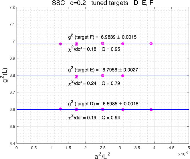
Figure 1: The statistical significance of precision tuning to three targeted gauge couplings D, E, F is shown by fitting a constant to each $g^{2}$ at the lower $L/a$ values of each step.

The statistical analysis of the renormalized gauge coupling and step $\beta$-function of the precision tuned runs followed [17] and used similar software. For each run, extended in length between 5,000 and 20,000 time units of molecular dynamics time, autocorrelation times were measured in two independent ways, using estimates from the autocorrelation function and from the Jackknife blocking procedure. Errors on the renormalized couplings were consistent from the two procedures and the one from autocorrelation functions is listed in Table 1. Each run went through thermalization segments which were not included in the analysis. For detection of residual thermalization effects the replica method of [17] was used in the analysis. All 26 runs passed Q value tests when mean values and statistical errors of the replica segments were compared for thermal and other variations.

The leading cutoff effects in the step function at finite bare coupling $g_{0}^{2}$ appear at $a^{2}/L^{2}$ order with $a^{4}/L^{4}$ and higher order corrections. In our earlier work [1] the linear dependence on $a^{2}/L^{2}$ was detected and fitted without including higher order corrections in reaching the continuum limit of the $\beta$-function. The high precision of the data allows for testing the $a^{4}/L^{4}$ correction term leading to small increases of the continuum $\beta$-function within one standard deviation in the SSC setup. This is illustrated in Figure 2 for targets D and F.

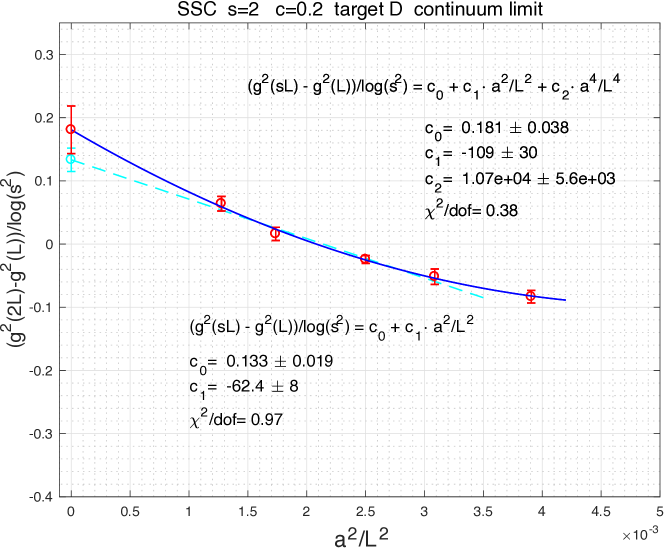
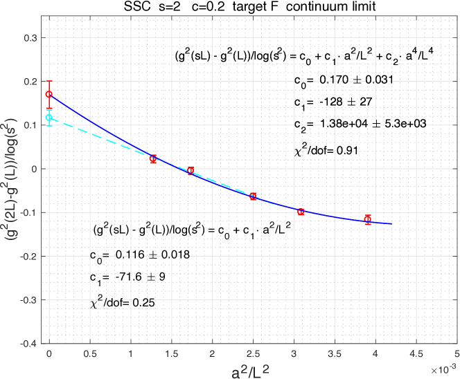
Figure 2: The consistency of extrapolations to the continuum $\beta$-function is illustrated comparing linear 3-point fits and quadratic 5-point fits in the $a^{2}/L^{2}$ variable for target D (top) and target F (bottom).

In addition to targeted precision tuning all the runs from the 6 targets A-F can be combined with additional trial runs from the tuning procedure into a new extended analysis which can project renormalized gauge couplings and step functions at any location in the bracketed range by using simple polynomial interpolation. Two samples of all the high quality polynomial interpolations are shown in Figure 3. This procedure allowed us to include the WSC analysis and the $c=0.25$ renormalization scheme in the new work.

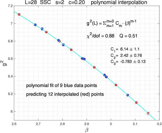
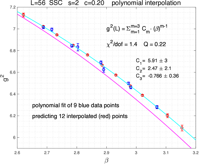
Figure 3: Polynomial interpolation is shown for 12 targeted gauge couplings (red points) using 9 inputs (blue points) from 6 runs of precision tuning and from additional auxiliary runs used in the tuning procedure. The largest $28\rightarrow 56$ step is shown with the magenta line marking the fit of the L=28 data (top) overlayed on the L=56 plot (bottom). The step $\beta$-function is positive throughout the targeted range.

The results shown in Figure 3 are quite remarkable. The largest $28\rightarrow 56$ step probes the smallest value of $a^{2}/L^{2}$ with a positive step $\beta$-function over the whole bracketed $g^{2}$ range, incompatible with a zero in the $\beta$-function as first evidence against the existence of the IRFP.

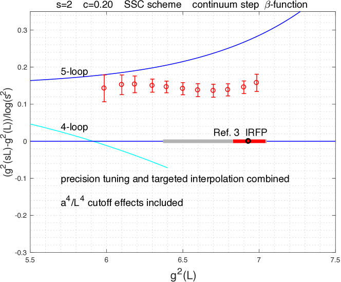
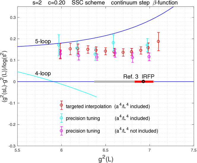
Figure 4: In the top panel results are shown using simple polynomial interpolation for 6 combined precision tuned target runs and 3 additional auxiliary runs. Fits in extrapolation of the steps include the $a^{4}/L^{4}$ cutoff effects as shown in Figure 5. The IRFP with red bar for statistical error and grey bar for systematic estimate is from [3]. The lower panel, with slightly shifted data in cyan and magenta colors for visibility, compares results from precision tuning and the combined method with an extrapolated point predicted slightly outside the bracketed interpolation range. Linear 3-point fits in $a^{2}/L^{2}$ were used for precision tuned targets A and B (4-point fits before in [1] ). Both plots display the 4-loop and recent 5-loop results referenced in the main text.

The main results of the SSC analysis of the $c=0.20$ renormalization scheme with step size $s=2$ are shown in Figure 4. The top panel of the figure is the outcome of the analysis from the combined use of the precision tuned 6 target runs and auxiliary runs using simple polynomial interpolation for 11 predictions which include the 6 locations of precision tuning for consistency and enhanced accuracy. The lower panel in Figure 4 compares results from precision tuning with the combined method showing remarkable consistency. Both the upper and lower panels display the 4-loop and recent 5-loop results of the continuum $\beta$-function in the $g_{\overline{\rm MS\kern-0.5pt}\kern 0.5pt}^{2}$ scheme [18, 19, 20, 21, 22]. Extrapolation of the steps from finite bare couplings $g_{0}^{2}$ to the continuum $\beta$-function includes the $a^{4}/L^{4}$ cutoff effects with typical fits shown in Figure 5.

In the 4-loop approximation the $n_{f}=12$ theory has an IRFP which disappears in the 5-loop approximation. The 5-loop $\beta$-function predicts the lower edge of the conformal window between $n_{f}=12$ and $n_{f}=13$. It will require further investigation to understand the potential significance of the apparent consistency between the 5-loop $\beta$-function and our simulation results in different renormalization schemes. The authors of [2, 3, 4] prefer to show only the 4-loop $\beta$-function which exhibits a zero at the $g^{2}$ location close to where the original IRFP was published in [2] before being relocated to $g^{2}\approx 7$ in the $c=0.20$ renormalization scheme [3, 4]. The 4-loop zero in the $\beta$-function is inconsistent with the new 5-loop results. Independently, and non-perturbatively, the reported IRFP is ruled out in our new analysis of the extended data set with overwhelming statistical significance as illustrated in Figure 4.

3.2 WSC gradient flow with c=0.20 renormalization scheme

The WSC setup in our analysis designates the replacement of the tree-level improved Symanzik action by the simple Wilson plaquette action to drive the gradient flow on the gauge configurations which were generated by the Symanzik action in the HMC evolution code. The $a^{4}/L^{4}$ cutoff contamination plays a critically important role in establishing consistency between the WSC scheme and the much less cutoff contaminated SSC scheme in reaching the correct continuum $\beta$-function. Since only the Wilson plaquette action was used for the gradient flow in [2, 3], the WSC analysis is useful for completeness and consistency checks. Figure 5 shows the consistency of the two gradient flows converging to the same continuum $\beta$-function in the $c=0.20$ renormalization scheme with step size $s=2$.

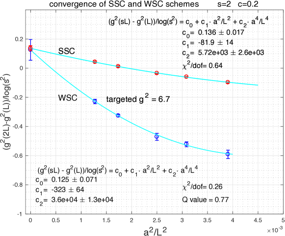
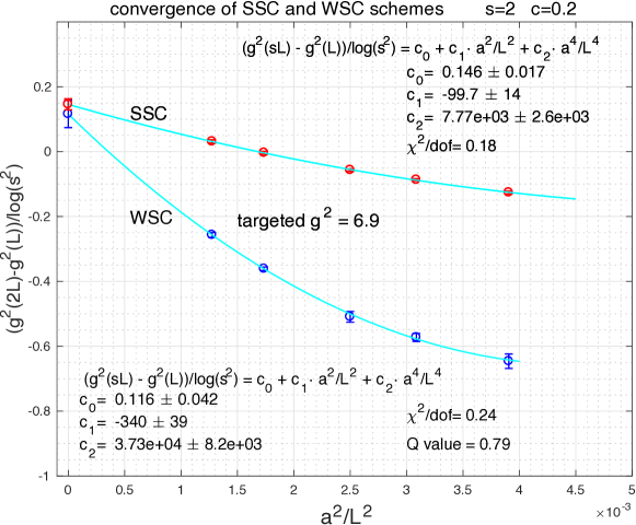
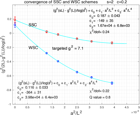
Figure 5: The fitting procedure is shown for SSC and WSC analyses where Symanzik action and Wilson action are driving the gauge field gradient flow respectively. The analysis of the extrapolation to the continuum $\beta$-function includes in both cases the $a^{2}/L^{2}$ and the $a^{4}/L^{4}$ terms in the fitting procedure.

The analysis of extrapolations to the continuum $\beta$-function included both the $a^{2}/L^{2}$ term and the $a^{4}/L^{4}$ term in the fitting procedure. It is quite remarkable that consistency is clearly established although the cutoff effects in the WSC gradient flow are almost an order of magnitude larger than in the SSC gradient flow.

The origin of the large WSC cutoff effects: The lattice implementation of composite operators gets renormalized along the gradient flow as a function of flow time $t$. Figure 6 shows the renormalization of the clover lattice implementation of the composite operator $E(t)=-\frac{1}{2}{\rm Tr}F_{\mu\nu}F_{\mu\nu}(t)$ along the gradient flow, proportional to $g^{2}(t)$ we target.

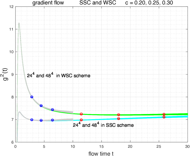
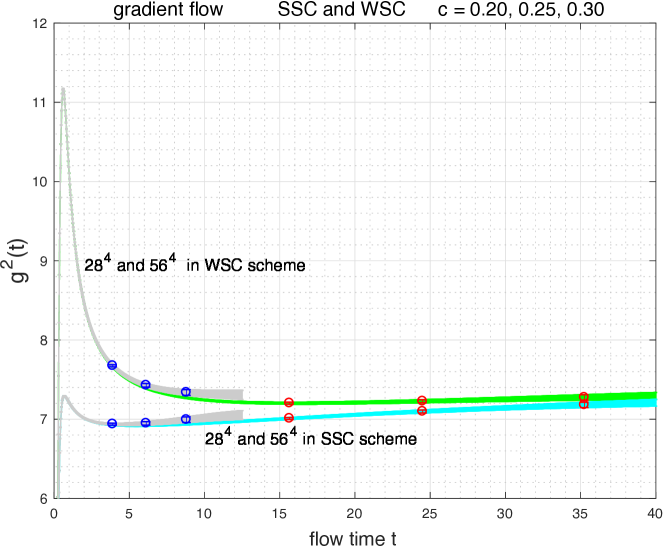
Figure 6: For renormalization schemes $c=0.20/0.25/0.30$, the locations of the paired points of the step $\beta$-functions are shown separately for Wilson and Symanzik action driving the gradient flow. Grey color shades the flow of the smaller $L$ of the pair with blue data points, green and cyan colors shade the larger $L$ with red data points. The top panel is the $24\rightarrow 48$ step, the lower panel shows the $28\rightarrow 56$ step. The target F set of Table 1 was used at all 3 values of $c$ for SSC and WSC.

The renormalization of the operator $E(t)$ goes through transient effects at short flow times before the cutoff effects get sufficiently renormalized. These transient effects are almost an order of magnitude larger along the Wilson flow for the same clover lattice implementation as used in the Symanzik flow. In our WSC approach, much larger stepped volumes would be needed to match the smaller cutoff effects in extrapolation of the SSC approach to the continuum $\beta$-function. This is clearly demonstrated in Figure 5 and in Figure 6. We do not see how the stronger cutoff dependence of the Wilson flow allows one to ignore the $a^{4}/L^{4}$ effects of small lattices when gauge and fermion actions different from ours are used in generating configurations in the simulations, like in [5, 6, 4].

3.3 The c=0.25 renormalization scheme

We also analyzed our data set in the $c=0.25$ renormalization scheme which is further away from the $c=0$ infinite volume scheme and less sensitive to cutoff effects. A subset of the full $c=0.25$ analysis is shown in Figure 7.

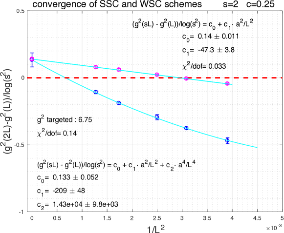
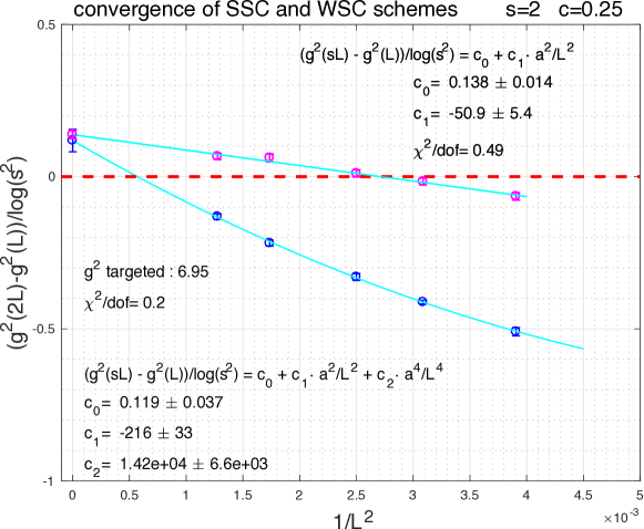
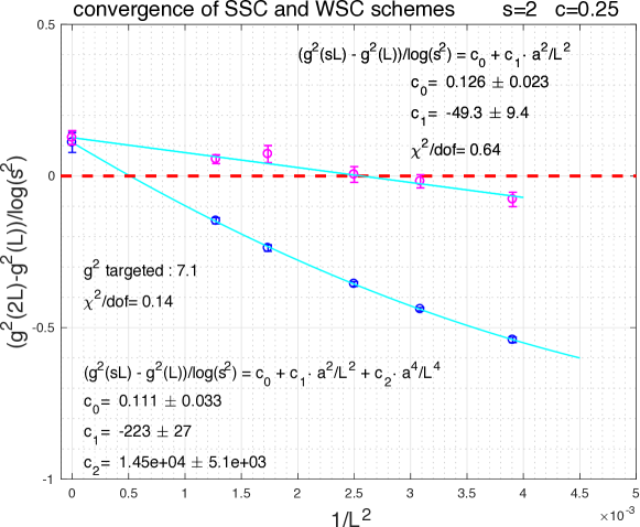
Figure 7: The fitting procedure is shown in the $c=0.25$ renormalization scheme for SSC and WSC analyses where Symanzik action and Wilson action are driving the gauge field gradient flow respectively. The analysis of the extrapolation to the continuum $\beta$-function includes $a^{2}/L^{2}$ and $a^{4}/L^{4}$ terms in the WSC fitting procedure.

We combine again all the runs from precision tuning of the 6 targets A-F with additional trial runs from the tuning procedure into a new extended analysis with SSC and WSC gradient flow and the $c=0.25$ renormalization scheme at step size $s=2$. In this new analysis we can predict again renormalized gauge couplings and step functions at any location in the bracketed range by using simple polynomial interpolation. Although the cutoff effect of the renormalization is much bigger when the Wilson action is driving the gradient flow, the two consistently converge to the same continuum $\beta$-function. The $\beta$-function in Figure 8 is consistent with the $c=0.20$ renormalization scheme and without any trace of the IRFP reported in [2, 3] for the $c=0.25$ renormalization scheme.

Figure 8: Results are shown for SSC $c=0.25$ with step size $s=2$ using simple polynomial interpolation for 6 combined precision tuned target runs and 3 additional auxiliary runs. Linear fits are used in the SSC analysis of the steps and the WSC analysis for cross checks includes $a^{4}/L^{4}$ cutoff effects as shown in Figure 7. The location of the IRFP in the $c=0.25$ scheme of [3] is somewhat shifted to the right from the location of the IRFP in the $c=0.20$ scheme as displayed in this figure and in Figure 4. The 4-loop and recent 5-loop results for the $\beta$-function are referenced in the main text.

4 Ten-flavor preview with conclusions

We explored SSC and WSC gradient flows in the $c=0.20$ and $c=0.25$ renormalization schemes for the determination of the continuum $\beta$-function with twelve flavors of massless fermions. Consistent results from our high precision simulations in large volumes do not show any infrared fixed point reported at several locations in [2, 3, 4]. This disagreement requires resolution and closure. Arguments were presented in [4] that the different results should not be viewed as disagreements in the simulations and in their analysis but as evidence for the violation of universality in the staggered formulation. Supporting this argument, three examples were invoked in [4]:

1. showing conformal fixed point structures in 3D statistical models with several fixed points,

2. disagreement between sextet $\beta$-functions using Wilson fermions [23] and rooted staggered fermions [24],

3. new results finding an IRFP with ten flavors of massless domain wall fermions implies conformal behavior for twelve flavors as well.

We note our disagreements in response:

1. Since staggered fermions at $n_{f}=12$ are built on a UV fixed point at zero gauge coupling, relevant or marginal operators, like in the examples of the 3D statistical models in [4], cannot be added to the staggered lattice fermion action which has correct locality and universality properties. The explicit construction is well-known in the literature. Besides, the controversy between [2, 3, 4] and our work exists for the staggered formulation itself.

2. The theoretical framework for the rooting procedure, without universality violation when the sextet gauge coupling is targeted in fixed physical volume, was explained in [24]. It has not been challenged since in any follow up to the original criticism [23].

3. We recently completed the comprehensive analysis of the theory with ten massless fermion flavors in the fundamental representation of the SU(3) color gauge group. An important result is shown in Figure 9 for the preview of the $\beta$-function with SSC analysis of the gradient flow in the $c=0.25$ renormalization scheme using step size $s=2$ [9]. Every detail of the ten-flavor analysis followed closely the procedure we implemented and used here for the analysis of the twelve-flavor model. Since rooting was used for ten flavors with staggered fermions, we tested the validity of the theoretical argument presented in [24]. The Dirac spectrum was closely analyzed in the runs and the expected behavior of the quartet structure was confirmed.

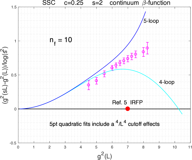
Figure 9: The IRFP as marked in the plot is taken from [5, 6], in complete disagreement with our analysis.

In conclusion, we find unacceptable the resolution of the problem as conjectured in [4].

References

- [1] Z. Fodor, K. Holland, J. Kuti, S. Mondal, D. Nogradi, C. H. Wong, Fate of the conformal fixed point with twelve massless fermions and SU(3) gauge group, Phys. Rev. D94 (9) (2016) 091501. arXiv:1607.06121, doi:10.1103/PhysRevD.94.091501.
- [2] A. Cheng, A. Hasenfratz, Y. Liu, G. Petropoulos, D. Schaich, Improving the continuum limit of gradient flow step scaling, JHEP 05 (2014) 137. arXiv:1404.0984, doi:10.1007/JHEP05(2014)137.
- [3] A. Hasenfratz, D. Schaich, Nonperturbative beta function of twelve-flavor SU(3) gauge theoryarXiv:1610.10004.
-
[4]
A. Hasenfratz, C. Rebbi, O. Witzel,
Testing
Fermion Universality at a Conformal Fixed Point, in: 35th International
Symposium on Lattice Field Theory (Lattice 2017) Granada, Spain, June 18-24,
2017, 2017.
arXiv:1708.03385.
URL https://inspirehep.net/record/1615760/files/arXiv:1708.03385.pdf - [5] T.-W. Chiu, The -function of gauge theory with massless fermions in the fundamental representationarXiv:1603.08854.
- [6] T.-W. Chiu, Discrete -function of the gauge theory with 10 massless domain-wall fermions, PoS LATTICE2016 (2017) 228.
- [7] T. Appelquist, G. T. Fleming, E. T. Neil, Lattice study of the conformal window in QCD-like theories, Phys. Rev. Lett. 100 (2008) 171607. doi:10.1103/PhysRevLett.100.171607.
- [8] T. Appelquist, G. T. Fleming, E. T. Neil, Lattice Study of Conformal Behavior in SU(3) Yang-Mills Theories, Phys. Rev. D79 (2009) 076010. arXiv:0901.3766, doi:10.1103/PhysRevD.79.076010.
- [9] Z. Fodor, K. Holland, J. Kuti, D. Nogradi, C. H. Wong, in preparation for publication.
- [10] R. Narayanan, H. Neuberger, Infinite N phase transitions in continuum Wilson loop operators, JHEP 03 (2006) 064. doi:10.1088/1126-6708/2006/03/064.
- [11] M. Lüscher, Properties and uses of the Wilson flow in lattice QCD, JHEP 08 (2010) 071. doi:10.1007/JHEP08(2010)071,10.1007/JHEP03(2014)092.
- [12] M. Luscher, Topology, the Wilson flow and the HMC algorithm, PoS LATTICE2010 (2010) 015. arXiv:1009.5877.
- [13] M. Luscher, P. Weisz, Perturbative analysis of the gradient flow in non-abelian gauge theories, JHEP 02 (2011) 051. doi:10.1007/JHEP02(2011)051.
- [14] R. Lohmayer, H. Neuberger, Continuous smearing of Wilson Loops, PoS LATTICE2011 (2011) 249. arXiv:1110.3522.
- [15] Z. Fodor, K. Holland, J. Kuti, D. Nogradi, C. H. Wong, The Yang-Mills gradient flow in finite volume, JHEP 11 (2012) 007. arXiv:1208.1051, doi:10.1007/JHEP11(2012)007.
- [16] M. Luscher, R. Narayanan, P. Weisz, U. Wolff, The Schrodinger functional: A Renormalizable probe for nonAbelian gauge theories, Nucl. Phys. B384 (1992) 168–228. arXiv:hep-lat/9207009, doi:10.1016/0550-3213(92)90466-O.
- [17] U. Wolff, Monte Carlo errors with less errors, Comput. Phys. Commun. 156 (2004) 143–153. doi:10.1016/S0010-4655(03)00467-3,10.1016/j.cpc.2006.12.001.
- [18] P. A. Baikov, K. G. Chetyrkin, J. H. Kühn, Five-Loop Running of the QCD coupling constant, Phys. Rev. Lett. 118 (8) (2017) 082002. arXiv:1606.08659, doi:10.1103/PhysRevLett.118.082002.
- [19] T. A. Ryttov, R. Shrock, Scheme-independent calculation of for an SU(3) gauge theory, Phys. Rev. D94 (10) (2016) 105014. arXiv:1608.00068, doi:10.1103/PhysRevD.94.105014.
- [20] T. A. Ryttov, R. Shrock, Higher-order scheme-independent series expansions of and in conformal field theories, Phys. Rev. D95 (10) (2017) 105004. arXiv:1703.08558, doi:10.1103/PhysRevD.95.105004.
- [21] T. Luthe, A. Maier, P. Marquard, Y. Schroder, Complete renormalization of QCD at five loops, JHEP 03 (2017) 020. arXiv:1701.07068, doi:10.1007/JHEP03(2017)020.
- [22] F. Herzog, B. Ruijl, T. Ueda, J. A. M. Vermaseren, A. Vogt, The five-loop beta function of Yang-Mills theory with fermions, JHEP 02 (2017) 090. arXiv:1701.01404, doi:10.1007/JHEP02(2017)090.
- [23] A. Hasenfratz, Y. Liu, C. Y.-H. Huang, The renormalization group step scaling function of the 2-flavor SU(3) sextet modelarXiv:1507.08260.
- [24] Z. Fodor, K. Holland, J. Kuti, S. Mondal, D. Nogradi, C. H. Wong, The running coupling of the minimal sextet composite Higgs model, JHEP 09 (2015) 039. arXiv:1506.06599, doi:10.1007/JHEP09(2015)039.