Gluing Delaunay ends to minimal $n$-noids using the DPW method

Abstract: we construct constant mean curvature surfaces in euclidean space by gluing $n$ half Delaunay surfaces to a non-degenerate minimal $n$-noid, using the DPW method.

1. Introduction

In [3], Dorfmeister, Pedit and Wu have shown that surfaces with non-zero constant mean curvature (CMC for short) in euclidean space admit a Weierstrass-type representation, which means that they can be represented in terms of holomorphic data. This representation is now called the DPW method. In [14], we used the DPW method to construct CMC $n$-noids: genus zero, CMC surfaces with $n$ ends Delaunay type ends. These $n$-noids can be described as a unit sphere with $n$ half Delaunay surfaces with small necksizes attached at prescribed points. They had already been constructed by Kapouleas in [8] using PDE methods.

In the case $n=3$, Alexandrov-embedded CMC trinoids have been classified by Große Brauckman, Kusner and Sullivan in [6]. In particular, equilateral CMC trinoids form a 1-parameter family, parametrized on an open interval. On one end, equilateral trinoids degenerate like the examples described above: they look like a sphere with 3 half Delaunay surfaces with small necksizes attached at the vertices of a spherical equilateral triangle. On the other end, equilateral trinoids limit, after suitable blow-up, to a minimal $3$-noid: a genus zero minimal surface with 3 catenoidal ends (see Figure 1).

It seems natural to ask if one can generalize this observation and construct CMC $n$-noids by gluing half Delaunay surfaces with small necksizes to a minimal $n$-noid. This is indeed the case, and has been done by Mazzeo and Pacard in [10] using PDE methods. In this paper, we propose a quite simple and natural DPW potential to construct these examples. We prove:

Theorem 1.

Let $n\geq 3$ and let $M_{0}$ be a non-degenerate minimal $n$-noid. There exists a smooth family of CMC surfaces $(M_{t})_{0<|t|<\epsilon}$ with the following properties:

1. $M_{t}$ has genus zero and $n$ Delaunay ends.

2. $\frac{1}{t}M_{t}$ converges to $M_{0}$ as $t\to 0$.

3. If $M_{0}$ is Alexandrov-embedded, all ends of $M_{t}$ are of unduloid type if $t>0$ and of nodoid type if $t<0$. Moreover, $M_{t}$ is Alexandrov-embedded if $t>0$.

Non-degeneracy of a minimal $n$-noid will be defined in Section 2. The two surfaces $M_{t}$ and $M_{-t}$ are geometrically different: if $M_{t}$ has an end of unduloid type then the corresponding end of $M_{-t}$ is of nodoid type. See Proposition 5 for more details.

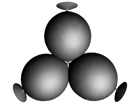
Figure 1. A CMC 3-noid (left, image by N. Schmitt [12]) and a minimal 3-noid (right). There is a tiny “copy” of the minimal 3-noid at the center of the CMC 3-noid.

Of course, a minimal $n$-noid is never embedded if $n\geq 3$ so the surfaces $M_{t}$ are not embedded. Alexandrov-embedded minimal $n$-noids whose ends have coplanar axes have been classified by Cosin and Ros in [2], and Alexandrov-embedded CMC $n$-noids whose ends have coplanar axes have been classified by Große-Brauckmann, Kusner and Sullivan in [7].

As already said, these surfaces have already been constructed in [10]. Our motivation to construct them with the DPW method is to answer the following questions:

1. How can we produce a DPW potential from the Weierstrass data $(g,\omega)$ of the minimal $n$-noid $M_{0}$ ?

2. How can we prove, with the DPW method, that $\frac{1}{t}M_{t}$ converges to $M_{0}$ ?

The answer to Question 2 is Theorem 4 in Section 4, a general blow-up result in the context of the DPW method. In [15], we use the DPW method to construct higher genus CMC surfaces with small necks. Theorem 4 is used to ensure that the necks have asymptotically catenoidal shape.

2. Non-degenerate minimal $n$-noids

A minimal $n$-noid is a complete, immersed minimal surface in ${\mathbb{R}}^{3}$ with genus zero and $n$ catenoidal ends. Let $M_{0}$ be a minimal $n$-noid and $(\Sigma,g,\omega)$ its Weierstrass data. This means that $M_{0}$ is parametrized on $\Sigma$ by the Weierstrass Representation formula:

(1) $$\psi(z)={\rm Re}\int_{z_{0}}^{z}\left(\mbox{$\frac{1}{2}$}(1-g^{2})\omega,\mbox{$\frac{{\rm i}}{2}$}(1+g^{2})\omega,g\omega\right)$$

Without loss of generality, we can assume that $\Sigma={\mathbb{C}}\cup\{\infty\}\setminus\{p_{1},\cdots,p_{n}\}$, where $p_{1},\cdots,p_{n}$ are complex numbers and $g\neq 0,\infty$ at $p_{1},\cdots,p_{n}$ (by rotating $M_{0}$ if necessary). Then $\omega$ needs a double pole at $p_{1},\cdots,p_{n}$ so has $2n-2$ zeros, counting multiplicity. Since $\omega$ needs a zero at each pole of $g$, with twice the multiplicity, it follows that $g$ has $n-1$ poles so has degree $n-1$. Hence we may write

(2) $$g=\frac{A(z)}{B(z)}\quad\mbox{ and }\quad\omega=\frac{B(z)^{2}\,dz}{\prod_{i=1}^{n}(z-p_{i})^{2}}$$

where

$$A(z)=\sum_{i=1}^{n}a_{i}z^{n-i}\quad\mbox{ and }\quad B(z)=\sum_{i=1}^{n}b_{i}z^{n-i}.$$

We are going to deform this Weierstrass data, so we see $a_{i}$, $b_{i}$ and $p_{i}$ for $1\leq i\leq n$ as complex parameters. We denote by ${\bf x}\in{\mathbb{C}}^{3n}$ the vector of these parameters, and by ${\bf x}_{0}$ the value of the parameters corresponding to the minimal $n$-noid $M_{0}$.

Let $\gamma_{i}$ be the homology class of a small circle centered at $p_{i}$ and define the following periods for $1\leq i\leq n$ and $0\leq k\leq 2$, depending on the parameter vector ${\bf x}\in{\mathbb{C}}^{3n}$:

$$P_{i,k}({\bf x})=\int_{\gamma_{i}}g^{k}\omega$$

$$P_{i}({\bf x})=(P_{i,0}({\bf x}),P_{i,1}({\bf x}),P_{i,2}({\bf x}))\in{\mathbb{C}}^{3}$$

$$Q_{i}({\bf x})=\int_{\gamma_{i}}\left(\mbox{$\frac{1}{2}$}(1-g^{2})\omega,\mbox{$\frac{{\rm i}}{2}$}(1+g^{2})\omega,g\omega\right)\in{\mathbb{C}}^{3}.$$

Then

$$Q_{i}({\bf x})=\left(\mbox{$\frac{1}{2}$}(P_{i,0({\bf x})}-P_{i,2}({\bf x})),\mbox{$\frac{{\rm i}}{2}$}(P_{i,0}({\bf x})+P_{i,2}({\bf x})),P_{i,1}({\bf x})\right).$$

The components of $Q_{i}({\bf x}_{0})$ are imaginary because the Period Problem is solved for $M_{0}$. This gives

(3) $$P_{i,2}({\bf x}_{0})=\overline{P_{i,0}({\bf x}_{0})}\quad\mbox{ and }\quad P_{i,1}({\bf x}_{0})\in{\rm i}{\mathbb{R}}$$

Moreover, ${\rm Im}(Q_{i}({\bf x}_{0}))=-\phi_{i}$ where $\phi_{i}$ is the flux vector of $M_{0}$ at the end $p_{i}$. By the Residue Theorem, we have for all ${\bf x}$ in a neighborhood of ${\bf x}_{0}$:

$$\sum_{i=1}^{n}P_{i}({\bf x})=0$$

Let $P=(P_{1},\cdots,P_{n-1})$ and $Q=(Q_{1},\cdots,Q_{n-1})$.

Definition 1.

$M_{0}$ is non-degenerate if the differential of $P$ (or equivalently, $Q$) at ${\bf x}_{0}$ has (complex) rank $3n-3$.

Remark 1.

If $n\geq 3$, we may (using Möbius transformations of the sphere) fix the value of three points, say $p_{1},p_{2},p_{3}$. Then "non-degenerate" means that the differential of $P$ with respect to the remaining parameters is an isomorphism of ${\mathbb{C}}^{3n-3}$.

This notion is related to another standard notion of non-degeneracy:

Definition 2.

$M_{0}$ is non-degenerate if its space of bounded Jacobi fields has (real) dimension 3.

Theorem 2.

If $M_{0}$ is non-degenerate in the sense of Definition 2, then $M_{0}$ is non-degenerate in the sense of Definition 1.

Proof. Assume $M_{0}$ is non-degenerate in the sense of Definition 2. Then in a neighborhood of $M_{0}$, the space ${\mathcal{M}}$ of minimal $n$-noids (up to translation) is a smooth manifold of dimension $3n-3$ by a standard application of the Implicit Function Theorem. Moreover, if we write $\phi_{i}\in{\mathbb{R}}^{3}$ for the flux vector at the $i$-th end, then the map $\phi=(\phi_{1},\cdots,\phi_{n})$ provides a local diffeomorphism between ${\mathcal{M}}$ and the space $V$ of vectors $v=(v_{1},\cdots,v_{n})\in({\mathbb{R}}^{3})^{n}$ such that $\sum_{i=1}^{n}v_{i}=0$. (All this is proved in Section 4 of [2] in the case where all ends are coplanar. The argument goes through in the general case.) Hence given a vector $v\in V$, there exists a deformation $M_{t}$ of $M_{0}$ such that $M_{t}\in{\mathcal{M}}$ and $\frac{d}{dt}\phi(M_{t})|_{t=0}=v$. We may write the Weierstrass data of $M_{t}$ as above and obtain a set of parameters ${\bf x}(t)$, depending smoothly on $t$, such that ${\bf x}(0)={\bf x}_{0}$. Then $dQ({\bf x}_{0})\cdot{\bf x}^{\prime}(0)=-{\rm i}v$. Since $Q$ is holomorphic, its differential is complex-linear so $dQ({\bf x}_{0})$ has complex rank equal to $\dim V=3n-3$. $\Box$

If all ends of $M_{0}$ have coplanar axes, then $M_{0}$ is non-degenerate in the sense of Definition 2 by Proposition 2 in [2]. In particular, the (most symmetric) $n$-noids of Jorge-Meeks are non-degenerate. This implies that generic $n$-noids in the component of the Jorge-Meeks $n$-noid are non-degenerate.

3. Background

In this section, we recall standard notations and results used in the DPW method. We work in the “untwisted” setting.

3.1. Loop groups

A loop is a smooth map from the unit circle ${\mathbb{S}}^{1}=\{\lambda\in{\mathbb{C}}:|\lambda|=1\}$ to a matrix group. The circle variable is denoted $\lambda$ and called the spectral parameter. For $\rho>0$, we denote ${\mathbb{D}}_{\rho}=\{\lambda\in{\mathbb{C}}\,:\,|\lambda|<\rho\}$, ${\mathbb{D}}_{\rho}^{*}={\mathbb{D}}_{\rho}\setminus\{0\}$ and ${\mathbb{D}}={\mathbb{D}}_{1}$.

• If $G$ is a matrix Lie group (or Lie algebra), $\Lambda G$ denotes the group (or algebra) of smooth maps $\Phi:{\mathbb{S}}^{1}\to G$.

• $\Lambda_{+}SL(2,{\mathbb{C}})\subset\Lambda SL(2,{\mathbb{C}})$ is the subgroup of maps $B$ which extend holomorphically to ${\mathbb{D}}$ with $B(0)$ upper triangular.

• $\Lambda_{+}^{{\mathbb{R}}}SL(2,{\mathbb{C}})\subset\Lambda_{+}SL(2,{\mathbb{C}})$ is the subgroup of maps $B$ such that $B(0)$ has positive entries on the diagonal.

Theorem 3 (Iwasawa decomposition).

The multiplication $\Lambda SU(2)\times\Lambda_{+}^{{\mathbb{R}}}SL(2,{\mathbb{C}})\to\Lambda SL(2,{\mathbb{C}})$ is a diffeomorphism. The unique splitting of an element $\Phi\in\Lambda SL(2,{\mathbb{C}})$ as $\Phi=FB$ with $F\in\Lambda SU(2)$ and $B\in\Lambda_{+}^{{\mathbb{R}}}SL(2,{\mathbb{C}})$ is called Iwasawa decomposition. $F$ is called the unitary factor of $\Phi$ and denoted $\mbox{\rm Uni}(\Phi)$. $B$ is called the positive factor and denoted $\mbox{\rm Pos}(\Phi)$.

3.2. The matrix model of ${\mathbb{R}}^{3}$

In the DPW method, one identifies ${\mathbb{R}}^{3}$ with the Lie algebra $\mathfrak{su}(2)$ by

$$x=(x_{1},x_{2},x_{3})\in{\mathbb{R}}^{3}\longleftrightarrow X=-{\rm i}\left(\begin{array}[]{cc}-x_{3}&x_{1}+{\rm i}x_{2}\\ x_{1}-{\rm i}x_{2}&x_{3}\end{array}\right)\in\mathfrak{su}(2).$$

We have $\det(X)=\|x\|^{2}$. The group $SU(2)$ acts as linear isometries on $\mathfrak{su}(2)$ by conjugation: $H\cdot X=HXH^{-1}$.

3.3. The DPW method

The input data for the DPW method is a quadruple $(\Sigma,\xi,z_{0},\phi_{0})$ where:

• $\Sigma$ is a Riemann surface.

• $\xi=\xi(z,\lambda)$ is a $\Lambda\mathfrak{sl}(2,{\mathbb{C}})$-valued holomorphic 1-form on $\Sigma$ called the DPW potential. More precisely,

  (4) $$\xi=\left(\begin{array}[]{cc}\alpha&\lambda^{-1}\beta\\ \gamma&-\alpha\end{array}\right)$$

  where $\alpha(z,\lambda)$, $\beta(z,\lambda)$, $\gamma(z,\lambda)$ are holomorphic 1-forms on $\Sigma$ with respect to the $z$ variable, and are holomorphic with respect to $\lambda$ in the disk ${\mathbb{D}}_{\rho}$ for some $\rho>1$.

• $z_{0}\in\Sigma$ is a base point.

• $\phi_{0}\in\Lambda SL(2,{\mathbb{C}})$ is an initial condition.

Given this data, the DPW method is the following procedure.

• Let $\widetilde{\Sigma}$ be the universal cover of $\Sigma$ and $\widetilde{z}_{0}\in\widetilde{\Sigma}$ be an arbitrary element in the fiber of $z_{0}$. Solve the Cauchy Problem on $\widetilde{\Sigma}$:

  (5) $$\left\{\begin{array}[]{l}d\Phi(z,\lambda)=\Phi(z,\lambda)\xi(z,\lambda)\\ \Phi(\widetilde{z}_{0},\lambda)=\phi_{0}(\lambda)\end{array}\right.$$

  to obtain a solution $\Phi:\widetilde{\Sigma}\to\Lambda SL(2,{\mathbb{C}})$.

• Compute the Iwasawa decomposition $(F(z,\cdot),B(z,\cdot))$ of $\Phi(z,\cdot)$.

• Define $f:\widetilde{\Sigma}\to\mathfrak{su}(2)\sim{\mathbb{R}}^{3}$ by the Sym-Bobenko formula:

  (6) $$f(z)=-2{\rm i}\frac{\partial F}{\partial\lambda}(z,1)F(z,1)^{-1}=:\mbox{\rm Sym}(F(z,\cdot)).$$

  Then $f$ is a CMC-1 (branched) conformal immersion. $f$ is regular at $z$ (meaning unbranched) if and only if $\beta(z,0)\neq 0$. Its Gauss map is given by

  (7) $$N(z)=-{\rm i}F(z,1)\left(\begin{array}[]{cc}-1&0\\ 0&1\end{array}\right)F(z,1)^{-1}=:\mbox{\rm Nor}(F(z,\cdot)).$$

  The differential of $f$ satisfies

  (8) $$df(z)=2{\rm i}\,B_{11}(z,0)^{2}F(z,1)\left(\begin{array}[]{cc}0&\beta(z,0)\\ \overline{\beta}(z,0)&0\end{array}\right)F(z,1)^{-1}.$$

Remark 2.

1. In [14], I have opposite signs in Equations (6) and (7). This is unfortunate because it makes the basis $(f_{x},f_{y},N)$ negatively oriented. Equation (6) is the right formula, which one obtains by untwisting the standard Sym-Bobenko formula in the twisted case. See [9] or [13].

2. I have not been able to find Formula (8) in the litterature. Of course, the DPW method constructs a moving frame for $f$, so one has a formula for $df$, but usually it is written in a special coordinate system and only in the “twisted” setting. For the interested reader, I derive Equation (8) from the Sym-Bobenko formula at the end of Appendix A.

3.4. The Monodromy Problem

Assume that $\Sigma$ is not simply connected so its universal cover $\widetilde{\Sigma}$ is not trivial. Let $\mbox{Deck}(\widetilde{\Sigma}/\Sigma)$ be the group of fiber-preserving diffeomorphisms of $\widetilde{\Sigma}$. For $\gamma\in\mbox{Deck}(\widetilde{\Sigma}/\Sigma)$, let

$${\mathcal{M}}_{\gamma}(\Phi)(\lambda)=\Phi(\gamma(z),\lambda)\Phi(z,\lambda)^{-1}$$

be the monodromy of $\Phi$ with respect to $\gamma$ (which is independent of $z\in\widetilde{\Sigma}$). The standard condition which ensures that the immersion $f$ descends to a well defined immersion on $\Sigma$ is the following system of equations, called the Monodromy Problem.

(9) $$\forall\gamma\in\mbox{Deck}(\widetilde{\Sigma}/\Sigma)\quad\left\{\begin{array}[]{lc}{\mathcal{M}}_{\gamma}(\Phi)\in\Lambda SU(2)&(i)\\ {\mathcal{M}}_{\gamma}(\Phi)(1)=\pm I_{2}&(ii)\\ \frac{\partial{\mathcal{M}}_{\gamma}(\Phi)}{\partial\lambda}(1)=0&(iii)\end{array}\right.$$

One can identify $\mbox{Deck}(\widetilde{\Sigma}/\Sigma)$ with the fundamental group $\pi_{1}(\Sigma,z_{0})$ (see for example Theorem 5.6 in [4]), so we will in general see $\gamma$ as an element of $\pi_{1}(\Sigma,z_{0})$. Under this identification, the monodromy of $\Phi$ with respect to $\gamma\in\pi_{1}(\Sigma,z_{0})$ is given by

$${\mathcal{M}}_{\gamma}(\Phi)(\lambda)=\Phi(\widetilde{\gamma}(1),\lambda)\Phi(\widetilde{\gamma}(0),\lambda)^{-1}$$

where $\widetilde{\gamma}:[0,1]\to\widetilde{\Sigma}$ is the lift of $\gamma$ such that $\widetilde{\gamma}(0)=\widetilde{z}_{0}$.

3.5. Gauging

Definition 3.

A gauge on $\Sigma$ is a map $G:\Sigma\to\Lambda_{+}SL(2,{\mathbb{C}})$ such that $G(z,\lambda)$ depends holomorphically on $z\in\Sigma$ and $\lambda\in{\mathbb{D}}_{\rho}$ for some $\rho>1$.

Let $\Phi$ be a solution of $d\Phi=\Phi\xi$ and $G$ be a gauge. Let $\widehat{\Phi}=\Phi\times G$. Then $\widehat{\Phi}$ and $\Phi$ define the same immersion $f$. This is called “gauging”. The gauged potential is

$$\widehat{\xi}=\widehat{\Phi}^{-1}d\widehat{\Phi}=G^{-1}\xi G+G^{-1}dG$$

and will be denoted $\xi\cdot G$, the dot denoting the action of the gauge group on the potential.

3.6. Functional spaces

We decompose a smooth function $f:{\mathbb{S}}^{1}\to{\mathbb{C}}$ in Fourier series

$$f(\lambda)=\sum_{i\in{\mathbb{Z}}}f_{i}\lambda^{i}$$

Fix some $\rho>1$ and define

$$\|f\|=\sum_{i\in{\mathbb{Z}}}|f_{i}|\rho^{|i|}$$

Let ${\mathcal{W}}_{\rho}$ be the space of functions $f$ with finite norm. This is a Banach algebra, classically called the Wiener algebra when $\rho=1$ (see Proposition 7 in appendix A). Functions in ${\mathcal{W}}_{\rho}$ extend holomorphically to the annulus $\frac{1}{\rho}<|\lambda|<\rho$.

We define ${\mathcal{W}}_{\rho}^{\geq 0}$, ${\mathcal{W}}_{\rho}^{>0}$, ${\mathcal{W}}_{\rho}^{\leq 0}$ and ${\mathcal{W}}_{\rho}^{<0}$ as the subspaces of functions $f$ such that $f_{i}=0$ for $i<0$, $i\leq 0$, $i>0$ and $i\geq 0$, respectively. Functions in ${\mathcal{W}}_{\rho}^{\geq 0}$ extend holomorphically to the disk ${\mathbb{D}}_{\rho}$ and satisfy $|f(\lambda)|\leq\|f\|$ for all $\lambda\in{\mathbb{D}}_{\rho}$. We write ${\mathcal{W}}^{0}\sim{\mathbb{C}}$ for the subspace of constant functions, so we have a direct sum ${\mathcal{W}}_{\rho}={\mathcal{W}}_{\rho}^{<0}\oplus{\mathcal{W}}^{0}\oplus{\mathcal{W}}_{\rho}^{>0}$. A function $f$ will be decomposed as $f=f^{-}+f^{0}+f^{+}$ with $(f^{-},f^{0},f^{+})\in{\mathcal{W}}_{\rho}^{<0}\times{\mathcal{W}}^{0}\times{\mathcal{W}}_{\rho}^{>0}$.

We define the star operator by

$$f^{*}(\lambda)=\overline{f\left(\frac{1}{\overline{\lambda}}\right)}=\sum_{i\in{\mathbb{Z}}}\overline{f_{-i}}\lambda^{i}$$

The involution $f\mapsto f^{*}$ exchanges ${\mathcal{W}}_{\rho}^{\geq 0}$ and ${\mathcal{W}}_{\rho}^{\leq 0}$. We have $\lambda^{*}=\lambda^{-1}$ and $c^{*}=\overline{c}$ if $c$ is a constant. A function $f$ is real on the unit circle if and only if $f=f^{*}$.

If $L$ is a loop group, we denote $L_{\rho}\subset L$ the subgroup of loops whose entries are in ${\mathcal{W}}_{\rho}$. If $\Phi\in\Lambda SL(2,{\mathbb{C}})_{\rho}$ and $(F,B)$ is its Iwasawa decomposition, then in fact $F\in\Lambda SU(2)_{\rho}$ and $B\in\Lambda_{+}^{{\mathbb{R}}}SL(2,{\mathbb{C}})_{\rho}$ (see Proposition 8 in Appendix A). Moreover, Iwasawa decomposition is smooth, as a map between Banach manifolds (see Theorem 5 in Appendix A).

4. A blow-up result

In this section, we consider a one-parameter family of DPW potential $\xi_{t}$ with solution $\Phi_{t}$ and assume that $\Phi_{0}(z,\lambda)$ is independent of $\lambda$. Then its unitary part $F_{0}(z,\lambda)$ is independent of $\lambda$. The Sym Bobenko formula yields that $f_{0}\equiv 0$, so the family $f_{t}$ collapses to the origin as $t=0$. The following theorem says that the blow-up $\frac{1}{t}f_{t}$ converges to a minimal surface whose Weierstrass data is explicitly computed.

Theorem 4.

Let $\Sigma$ be a Riemann surface, $(\xi_{t})_{t\in I}$ a family of DPW potentials on $\Sigma$ and $(\Phi_{t})_{t\in I}$ a family of solutions of $d\Phi_{t}=\Phi_{t}\xi_{t}$ on the universal cover $\widetilde{\Sigma}$ of $\Sigma$, where $I\subset{\mathbb{R}}$ is a neighborhood of $0$. Fix a base point $z_{0}\in\widetilde{\Sigma}$. Assume that

1. $(t,z)\mapsto\xi_{t}(z,\cdot)$ and $t\mapsto\Phi_{t}(z_{0},\cdot)$ are $C^{1}$ maps into $\Lambda\mathfrak{sl}(2,{\mathbb{C}})_{\rho}$ and $\Lambda SL(2,{\mathbb{C}})_{\rho}$, respectively.

2. For all $t\in I$, $\Phi_{t}$ solves the Monodromy Problem (9).

3. $\Phi_{0}(z,\lambda)$ is independent of $\lambda$:

   $$\Phi_{0}(z,\lambda)=\left(\begin{array}[]{cc}a(z)&b(z)\\ c(z)&d(z)\end{array}\right)$$

Let $f_{t}=\mbox{\rm Sym}(\mbox{\rm Uni}(\Phi_{t})):\Sigma\to{\mathbb{R}}^{3}$ be the CMC-1 immersion given by the DPW method. Then

$$\lim_{t\to 0}\frac{1}{t}f_{t}(z)=\psi(z)$$

where $\psi:\Sigma\to{\mathbb{R}}^{3}$ is a (possibly branched) minimal immersion with the following Weierstrass data:

$$g(z)=\frac{-a(z)}{c(z)}\quad\mbox{ and }\quad\omega=4c(z)^{2}\frac{\partial\xi_{t;12}^{(-1)}}{\partial t}|_{t=0}.$$

The limit is for the uniform $C^{1}$ convergence on compact subsets of $\Sigma$.

Here $\xi_{t;12}^{(-1)}$ denotes the coefficient of $\lambda^{-1}$ in the upper right entry of $\xi_{t}$. In case $\omega=0$, the minimal immersion degenerates into a point and $\psi$ is constant.

Proof: by standard ODE theory, $(t,z)\mapsto\Phi_{t}(z,\cdot)$ is a $C^{1}$ map into $\Lambda SL(2,{\mathbb{C}})_{\rho}$. Let $(F_{t},B_{t})$ be the Iwasawa decomposition of $\Phi_{t}$. By Theorem 5 in Appendix A, $(t,z)\mapsto F_{t}(z,\cdot)$ and $(t,z)\mapsto B_{t}(z,\cdot)$ are $C^{1}$ maps into $\Lambda SU(2)_{\rho}$ and $\Lambda_{+}^{{\mathbb{R}}}SL(2,{\mathbb{C}})_{\rho}$, respectively. At $t=0$, $\Phi_{0}$ is constant with respect to $\lambda$, so its Iwasawa decomposition is the standard $QR$ decomposition:

$$F_{0}=\frac{1}{\sqrt{|a|^{2}+|c|^{2}}}\left(\begin{array}[]{cc}a&-\overline{c}\\ c&\overline{a}\end{array}\right)\qquad B_{0}=\frac{1}{\sqrt{|a|^{2}+|c|^{2}}}\left(\begin{array}[]{cc}|a|^{2}+|c|^{2}&\overline{a}b+\overline{c}d\\ 0&1\end{array}\right).$$

The Sym-Bobenko formula (6) yields $f_{0}=0$. Let $\mu_{t}=B_{t;11}^{0}$ and $\beta_{t}=\xi_{t;12}^{(-1)}$. By Equation (8), we have

$$df_{t}(z)=2{\rm i}\,\mu_{t}(z)^{2}F_{t}(z,1)\left(\begin{array}[]{cc}0&\beta_{t}(z)\\ \overline{\beta}_{t}(z)&0\end{array}\right)F_{t}(z,1)^{-1}.$$

Hence $(t,z)\mapsto df_{t}(z)$ is a $C^{1}$ map. At $t=0$, $\xi_{0}$ is constant with respect to $\lambda$, so $\beta_{0}=0$. Define $\widetilde{f}_{t}(z)=\frac{1}{t}f_{t}(z)$ for $t\neq 0$. Then $d\widetilde{f}_{t}(z)$ extends at $t=0$, as a continous function of $(t,z)$, by

$$d\widetilde{f}_{0}=\frac{d}{dt}df_{t}|_{t=0} = 2{\rm i}\left(\begin{array}[]{cc}a&-\overline{c}\\ c&\overline{a}\end{array}\right)\left(\begin{array}[]{cc}0&\beta^{\prime}\\ \overline{\beta^{\prime}}&0\end{array}\right)\left(\begin{array}[]{cc}\overline{a}&\overline{c}\\ -c&a\end{array}\right)$$

$$= 2{\rm i}\left(\begin{array}[]{cc}-ac\beta^{\prime}-\overline{ac\beta^{\prime}}&a^{2}\beta^{\prime}-\overline{c^{2}\beta^{\prime}}\\ \overline{a^{2}\beta^{\prime}}-c^{2}\beta^{\prime}&ac\beta^{\prime}+\overline{ac\beta^{\prime}}\end{array}\right)$$

where $\beta^{\prime}=\frac{d}{dt}\beta_{t}|_{t=0}$. In euclidean coordinates, this gives

$$d\widetilde{f}_{0}=4\;{\rm Re}\left[\mbox{$\frac{1}{2}$}(c^{2}-a^{2})\beta^{\prime},\mbox{$\frac{{\rm i}}{2}$}(c^{2}+a^{2})\beta^{\prime},-ac\beta^{\prime}\right].$$

Writing $g=\frac{-a}{c}$ and $\omega=4c^{2}\beta^{\prime}$, we obtain

$$\widetilde{f}_{0}(z)=\widetilde{f}_{0}(z_{0})+{\rm Re}\int_{z_{0}}^{z}\left[\mbox{$\frac{1}{2}$}(1-g^{2})\omega,\mbox{$\frac{{\rm i}}{2}$}(1+g^{2})\omega,g\omega\right]$$

and we see that $\widetilde{f}_{0}$ is a minimal surface with Weierstrass data $(g,\omega)$. The last statement of Theorem 4 comes from the fact that $d\widetilde{f}_{t}$ converges uniformly to $d\widetilde{f}_{0}$ on compact subsets of $\Sigma$.

4.1. Example

As an example, we consider the family of Delaunay surfaces given by the following DPW potential in ${\mathbb{C}}^{*}$:

$$\xi_{t}(z,\lambda)=\left(\begin{array}[]{cc}0&\lambda^{-1}r+s\\ \lambda r+s&0\end{array}\right)\frac{dz}{z}\quad\mbox{ with }\quad\left\{\begin{array}[]{l}r+s=\frac{1}{2}\\ rs=t\\ r<s\end{array}\right.$$

with initial condition $\Phi_{t}(1)=I_{2}$. As $t\to 0$, we have $(r,s)\to(0,\frac{1}{2})$. We have

$$\Phi_{0}(z,\lambda)=\exp\left(\begin{array}[]{cc}0&\frac{1}{2}\\ \frac{1}{2}&0\end{array}\right)\log z=\frac{1}{2\sqrt{z}}\left(\begin{array}[]{cc}z+1&z-1\\ z-1&z+1\end{array}\right)$$

$$\frac{\partial\xi_{t}}{\partial t}|_{t=0}=\left(\begin{array}[]{cc}0&2\lambda^{-1}\\ 2\lambda&0\end{array}\right)\frac{dz}{z}.$$

Theorem 4 applies and gives

$$g(z)=\frac{1+z}{1-z}\quad\mbox{ and }\quad\omega(z)=4\left(\frac{z-1}{2\sqrt{z}}\right)^{2}\frac{2\,dz}{z}=2\left(\frac{z-1}{z}\right)^{2}dz.$$

This is the Weierstrass data of a horizontal catenoid of waist-radius 4 and axis $Ox_{1}$, with $x_{1}\to+\infty$ at the end $z=0$.

5. The DPW potential

We now start the proof of Theorem 1. Let $(g,\omega)$ be the Weierstrass data of the given minimal $n$-noid $M_{0}$, written as in Section 2. We introduce $3n$ $\lambda$-dependent parameters $a_{i}$, $b_{i}$ and $p_{i}$ for $1\leq i\leq n$ in the functional space ${\mathcal{W}}_{\rho}^{\geq 0}$. The vector of these parameters is denoted ${\bf x}\in({\mathcal{W}}_{\rho}^{\geq 0})^{3n}$. The parameter ${\bf x}$ is in a neighborhood of a (constant) central value ${\bf x}_{0}\in({\mathcal{W}}^{0})^{3n}$ which correspond to the Weierstrass data of $M_{0}$, written as in Section 2. We define

$$A_{{\bf x}}(z,\lambda)=\sum_{i=1}^{n}a_{i}(\lambda)z^{n-i}$$

$$B_{{\bf x}}(z,\lambda)=\sum_{i=1}^{n}b_{i}(\lambda)z^{n-i}$$

(12) $$g_{{\bf x}}(z,\lambda)=\frac{A_{{\bf x}}(z,\lambda)}{B_{{\bf x}}(z,\lambda)}$$

(13) $$\omega_{{\bf x}}(z,\lambda)=\frac{B_{{\bf x}}(z,\lambda)^{2}\,dz}{\prod_{i=1}^{n}(z-p_{i}(\lambda))^{2}}.$$

For $t$ in a neighborhood of $0$ in ${\mathbb{R}}$, we consider the following DPW potential:

$$\xi_{t,{\bf x}}(z,\lambda)=\left(\begin{array}[]{cc}0&\mbox{$\frac{1}{4}$}t(\lambda-1)^{2}\lambda^{-1}\omega_{{\bf x}}(z,\lambda)\\ dg_{{\bf x}}(z,\lambda)&0\end{array}\right).$$

We fix a base point $z_{0}$, away from the poles of $g$ and $\omega$, and we take the initial condition

$$\phi_{0}(\lambda)=\left(\begin{array}[]{cc}g_{{\bf x}}(z_{0},\lambda)&1\\ -1&0\end{array}\right).$$

These choices are motivated by the following observations:

1. At $t=0$, we have

   $$\xi_{0,{\bf x}}(z,\lambda)=\left(\begin{array}[]{cc}0&0\\ dg_{{\bf x}}(z,\lambda)&0\end{array}\right).$$

   The solution of the Cauchy Problem (5) is given by

   (14) $$\Phi_{0,{\bf x}}(z,\lambda)=\left(\begin{array}[]{cc}g_{{\bf x}}(z,\lambda)&1\\ -1&0\end{array}\right)$$

   which is well-defined, so the Monodromy Problem (9) is solved at $t=0$.

2. The same conclusion holds if $\lambda=1$ instead of $t=0$. In particular, Items (ii) and (iii) of the Monodromy Problem (9) are automatically solved.

3. At ${\bf x}={\bf x}_{0}$, we have $g_{{\bf x}_{0}}=g$ so $\Phi_{0,{\bf x}_{0}}(z,\lambda)$ is independent of $\lambda$. Moreover,

   $$\frac{\partial\xi_{t,{\bf x}_{0};12}^{(-1)}}{\partial t}|_{t=0}=\frac{\omega}{4}.$$

   Provided the Monodromy Problem is solved for all $t$ in a neighborhood of $0$, Theorem 4 applies and the limit minimal surface has Weierstrass data $(g,\omega)$ so is the minimal $n$-noid $M_{0}$, up to translation (see details in Section 7.1).

5.1. Regularity

Our potential $\xi_{t,{\bf x}}$ has poles at the zeros of $B_{{\bf x}}$ and the points $p_{1},\cdots,p_{n}$. (At $\infty$, we have $\omega_{{\bf x}}\sim b_{1}^{2}z^{-2}dz$ which is holomorphic.) We want the zeros of $B_{{\bf x}}$ to be apparent singularities, so we require the potential to be gauge-equivalent to a regular potential in a neighborhood of these points. Consider the gauge

$$G_{{\bf x}}(z,\lambda)=\left(\begin{array}[]{cc}g_{{\bf x}}(z,\lambda)^{-1}&-1\\ 0&g_{{\bf x}}(z,\lambda)\end{array}\right)$$

The gauged potential is

$$\widehat{\xi}_{t,{\bf x}}:=\xi_{t,{\bf x}}\cdot G_{{\bf x}}=\left(\begin{array}[]{cc}0&\mbox{$\frac{1}{4}$}t(\lambda-1)^{2}\lambda^{-1}g_{{\bf x}}^{2}\omega_{{\bf x}}\\ g_{{\bf x}}^{-2}dg_{{\bf x}}&0\end{array}\right).$$

We have

$$g_{{\bf x}}^{-2}dg_{{\bf x}}=\frac{A_{{\bf x}}^{\prime}B_{{\bf x}}-A_{{\bf x}}B_{{\bf x}}^{\prime}}{A_{{\bf x}}^{2}}\quad\mbox{ and }\quad g_{{\bf x}}^{2}\omega_{{\bf x}}=\frac{A_{{\bf x}}^{2}\,dz}{\prod_{i=1}^{n}(z-p_{i})^{2}}.$$

Let $\zeta$ be a zero of $B_{{\bf x}_{0}}$ (recall that $B_{{\bf x}_{0}}$ does not depend on $\lambda$). Then $A_{{\bf x}_{0}}(\zeta)\neq 0$. By continuity, there exists a neighborhood $U$ of $\zeta$ such that for $z\in U$, $\lambda\in{\mathbb{D}}_{\rho}$ and ${\bf x}$ close enough to ${\bf x}_{0}$, $A_{{\bf x}}(z,\lambda)\neq 0$. So $\widehat{\xi}_{t,{\bf x}}$ is holomorphic in $U\times{\mathbb{D}}_{\rho}^{*}$ and moreover, $\widehat{\xi}_{t,{\bf x};12}^{(-1)}\neq 0$. This ensures that the immersion extends analytically to $U$ and is unbranched in $U$.

6. The monodromy problem

6.1. Formulation of the problem

For $i\in[1,n]$, we denote $p_{i,0}$ the central value of the parameter $p_{i}$ (so $p_{1,0},\cdots,p_{n,0}$ are the ends of the minimal $n$-noid $M_{0}$). We consider the following $\lambda$-independent domain on the Riemann sphere:

(15) $$\Omega=\{z\in{\mathbb{C}}:\forall i\in[1,n],|z-p_{i,0}|>\varepsilon\}\cup\{\infty\}$$

where $\varepsilon>0$ is a fixed, small enough number such that the disks $D(p_{i,0},8\varepsilon)$ for $1\leq i\leq n$ are disjoint. As in [14], we first construct a family of immersions $f_{t}$ on $\Omega$. Then we extend $f_{t}$ to an $n$-punctured sphere in Proposition 3.

Let $\widetilde{\Omega}$ be the universal cover of $\Omega$ and $\Phi_{t,{\bf x}}(z,\lambda)$ be the solution of the following Cauchy Problem on $\widetilde{\Omega}$:

(16) $$\left\{\begin{array}[]{l}d\Phi_{t,{\bf x}}(z,\lambda)=\Phi_{t,{\bf x}}(z,\lambda)\xi_{t,{\bf x}}(z,\lambda)\\ \Phi_{t,{\bf x}}(\widetilde{z}_{0},\lambda)=\phi_{0}\end{array}\right.$$

We denote $\gamma_{1},\cdots,\gamma_{n-1}$ a set of generators of the fundamental group $\pi_{1}(\Omega,z_{0})$, with $\gamma_{i}$ encircling the point $p_{i,0}$. We may assume that each $\gamma_{i}$ is represented by a fixed curve avoiding the poles of $\xi_{t,{\bf x}}$. Let

$$M_{i}(t,{\bf x})={\mathcal{M}}_{\gamma_{i}}(\Phi_{t,{\bf x}})$$

be the monodromy of $\Phi_{t,{\bf x}}$ along $\gamma_{i}$. By Equation (14), we have $M_{i}(0,{\bf x})=I_{2}$. Recall that the matrix exponential is a local diffeomorphism from a neighborhood of $0$ in the Lie algebra $\mathfrak{sl}(2,{\mathbb{C}})$ (respectively $\mathfrak{su}(2)$) to a neighborhood of $I_{2}$ in $SL(2,{\mathbb{C}})$ (respectively $SU(2)$). The inverse diffeomorphism is denoted $\log$. For $t\neq 0$ small enough and $\lambda\in{\mathbb{D}}_{\rho}\setminus\{1\}$, we define as in [14]

$$\widetilde{M}_{i}(t,{\bf x})(\lambda)=\frac{4\lambda}{t(\lambda-1)^{2}}\log M_{i}(t,{\bf x})(\lambda).$$

Proposition 1.

1. $\widetilde{M}_{i}(t,{\bf x})(\lambda)$ extends smoothly at $t=0$ and $\lambda=1$, and each entry $\widetilde{M}_{i;k\ell}$ is a smooth map from a neighborhood of $(0,{\bf x}_{0})$ in ${\mathbb{R}}\times({\mathcal{W}}_{\rho}^{\geq 0})^{3}$ to ${\mathcal{W}}_{\rho}$.

2. At $t=0$, we have

   (17) $$\widetilde{M}_{i}(0,{\bf x})(\lambda)=\left(\begin{array}[]{cc}{\mathcal{P}}_{i,1}({\bf x})&{\mathcal{P}}_{i,2}({\bf x})\\ -{\mathcal{P}}_{i,0}({\bf x})&-{\mathcal{P}}_{i,1}({\bf x})\end{array}\right)\quad\mbox{ where }{\mathcal{P}}_{i,k}({\bf x})=\int_{\gamma_{i}}g_{{\bf x}}^{k}\omega_{{\bf x}}.$$

3. The Monodromy Problem (9) is equivalent to

   (18) $$\widetilde{M}_{i}(t,{\bf x})\in\Lambda\mathfrak{su}(2)\quad\mbox{ for }\quad 1\leq i\leq n-1.$$

Proof: we follow the proof of Proposition 1 in [14]. We first consider the case where the parameter ${\bf x}=(a_{i},b_{i},p_{i})_{1\leq i\leq n}$ is constant with respect to $\lambda$, so ${\bf x}\in{\mathbb{C}}^{3n}$. For $(\mu,{\bf x})$ in a neighborhood of $(0,{\bf x}_{0})$ in ${\mathbb{C}}\times{\mathbb{C}}^{3n}$, we define

$$\widehat{\xi}_{\mu,{\bf x}}(z)=\left(\begin{array}[]{cc}0&\mu\,\omega_{{\bf x}}(z)\\ dg_{{\bf x}}(z)&0\end{array}\right)$$

where $\omega_{{\bf x}}$ and $g_{{\bf x}}$ are defined by Equations (12) and (13), except that $a_{i}$, $b_{i}$, $p_{i}$ are constant complex numbers. Let $\widehat{\Phi}_{\mu,{\bf x}}$ be the solution of the Cauchy Problem $d\widehat{\Phi}_{\mu,{\bf x}}=\widehat{\Phi}_{\mu,{\bf x}}\widehat{\xi}_{\mu,{\bf x}}$ in $\widetilde{\Omega}$ with initial condition $\widehat{\Phi}_{\mu,{\bf x}}(\widetilde{z}_{0})=\phi_{0}$. Let $N_{i}(\mu,{\bf x})={\mathcal{M}}_{\gamma_{i}}(\widehat{\Phi}_{\mu,{\bf x}})$. By standard ODE theory, each entry of $N_{i}$ is a holomorphic function of $(\mu,{\bf x})$. At $\mu=0$, $\widehat{\Phi}_{0,{\bf x}}$ is given by Equation (14), so in particular $N_{i}(0,{\bf x})=I_{2}$. Hence

$$\widetilde{N}_{i}(\mu,{\bf x}):=\frac{1}{\mu}\log N_{i}(\mu,{\bf x})$$

extends holomorphically at $\mu=0$ with value $\widetilde{N}_{i}(0,{\bf x})=\frac{\partial N_{i}}{\partial\mu}(0,{\bf x})$. By Proposition 8 in Appendix A of [14],

$$\frac{\partial N_{i}}{\partial\mu}(0,{\bf x})=\int_{\gamma_{i}}\widehat{\Phi}_{0,{\bf x}}\frac{\partial\widehat{\xi}_{\mu,{\bf x}}}{\partial\mu}|_{\mu=0}\widehat{\Phi}_{0,{\bf x}}^{-1}.$$

Hence

(19) $$\widetilde{N}_{i}(0,{\bf x})=\int_{\gamma_{i}}\left(\begin{array}[]{cc}g_{{\bf x}}&1\\ -1&0\end{array}\right)\left(\begin{array}[]{cc}0&\omega_{{\bf x}}\\ 0&0\end{array}\right)\left(\begin{array}[]{cc}0&-1\\ 1&g_{{\bf x}}\end{array}\right)=\int_{\gamma_{i}}\left(\begin{array}[]{cc}g_{{\bf x}}\omega_{{\bf x}}&g_{{\bf x}}^{2}\omega_{{\bf x}}\\ -\omega_{{\bf x}}&-g_{{\bf x}}\omega_{{\bf x}}\end{array}\right).$$

For $(t,{\bf x})$ in a neighborhood of $(0,{\bf x}_{0})$ in ${\mathbb{R}}\times({\mathcal{W}}_{\rho}^{\geq 0})^{3n}$, we have

$$\xi_{t,{\bf x}}(z,\lambda)=\widehat{\xi}_{\mu(t,\lambda),{\bf x}(\lambda)}(z)\quad\mbox{ with }\quad\mu(t,\lambda)=\frac{t(\lambda-1)^{2}}{4\lambda}.$$

Hence

$$M_{i}(t,{\bf x})(\lambda)=N_{i}(\mu(t,\lambda),{\bf x}(\lambda))\quad\mbox{ and }\quad\widetilde{M}_{i}(t,{\bf x})(\lambda)=\widetilde{N}_{i}(\mu(t,\lambda),{\bf x}(\lambda)).$$

By substitution (see Proposition 9 in Appendix B of [14]), each entry of $\widetilde{M}_{i}$ is is a smooth map from a neighborhood of $(0,{\bf x}_{0})$ in ${\mathbb{R}}\times({\mathcal{W}}_{\rho}^{\geq 0})^{3}$ to ${\mathcal{W}}_{\rho}$. Moreover, $\widetilde{M}_{i}(0,{\bf x})$ is given by Equation (19). The fact that $\widetilde{M}_{i}$ extends holomorphically at $\lambda=1$ implies that Points (ii) and (iii) of Problem (9) are automatically satisfied. Since $\lambda^{-1}(\lambda-1)^{2}\in{\mathbb{R}}$ for $\lambda\in{\mathbb{S}}^{1}$, Equation (i) of Problem (9) is equivalent to Equation (18). $\Box$

6.2. Solution of the monodromy problem

Without loss of generality, we may (using a Möbius transformation of the sphere) fix the value of $p_{1}$, $p_{2}$ and $p_{3}$. We still denote ${\bf x}\in({\mathcal{W}}_{\rho}^{\geq 0})^{3n-3}$ the vector of the remaining parameters.

Proposition 2.

Assume that the given minimal $n$-noid is non-degenerate. For $t$ in a neighborhood of $0$, there exists a smooth function ${\bf x}(t)\in({\mathcal{W}}_{\rho}^{\geq 0})^{3n-3}$ such that $\widetilde{M}_{i}(t,{\bf x}(t),\cdot)\in\Lambda\mathfrak{su}(2)$ for $1\leq i\leq n-1$. Moreover, ${\bf x}(0)={\bf x}_{0}$.

Proof: recalling the definition of $P_{i,k}$ in Section 2 and ${\mathcal{P}}_{i,k}$ in Equation (17), we have

$${\mathcal{P}}_{i,k}({\bf x})(\lambda)=P_{i,k}({\bf x}(\lambda)).$$

Hence ${\mathcal{P}}_{i,k}$ is a smooth map from a neighborhood of ${\bf x}_{0}$ in $({\mathcal{W}}_{\rho}^{\geq 0})^{3n-3}$ to ${\mathcal{W}}_{\rho}^{\geq 0}$. Moreover, since ${\bf x}_{0}$ is constant, we have for $X\in({\mathcal{W}}_{\rho}^{\geq 0})^{3n-3}$:

(20) $$(d{\mathcal{P}}_{i,k}({\bf x}_{0})X)(\lambda)=dP_{i,k}({\bf x}_{0})X(\lambda).$$

Let ${\mathcal{P}}_{i}=({\mathcal{P}}_{i,0},{\mathcal{P}}_{i,1},{\mathcal{P}}_{i,2})$ and ${\mathcal{P}}=({\mathcal{P}}_{1},\cdots,{\mathcal{P}}_{n-1})$. By the non-degeneracy hypothesis and Remark 1, $dP({\bf x}_{0})$ is an automorphism of ${\mathbb{C}}^{3n-3}$, so $d{\mathcal{P}}({\bf x}_{0})$ is an automorphism of $({\mathcal{W}}_{\rho}^{\geq 0})^{3n-3}$ and restricts to an automorphism of $({\mathcal{W}}_{\rho}^{>0})^{3n-3}$.

We define the following smooth maps with value in ${\mathcal{W}}_{\rho}$ (the star operator is defined in Section 3.6)

$${\mathcal{F}}_{i}(t,{\bf x})=\widetilde{M}_{i,11}(t,{\bf x})+\widetilde{M}_{i,11}(t,{\bf x})^{*}$$

$${\mathcal{G}}_{i}(t,{\bf x})=\widetilde{M}_{i,12}(t,{\bf x})+\widetilde{M}_{i,21}(t,{\bf x})^{*}$$

Problem (18) is equivalent to ${\mathcal{F}}_{i}={\mathcal{G}}_{i}=0$. Actually, by definition, ${\mathcal{F}}_{i}={\mathcal{F}}_{i}^{*}$, so Problem (18) is equivalent to

$${\mathcal{F}}_{i}(t,{\bf x})^{+}=0,\quad{\rm Re}({\mathcal{F}}_{i}(t,{\bf x})^{0})=0\quad\mbox{ and }{\mathcal{G}}_{i}(t,{\bf x})=0\quad\mbox{ for $1\leq i\leq n-1$.}$$

At $t=0$, we have by Equation (17):

$${\mathcal{F}}_{i}(0,{\bf x})={\mathcal{P}}_{i,1}({\bf x})+{\mathcal{P}}_{i,1}({\bf x})^{*}$$

$${\mathcal{G}}_{i}(0,{\bf x})={\mathcal{P}}_{i,2}({\bf x})-{\mathcal{P}}_{i,0}({\bf x})^{*}$$

Equation (3) tells us precisely that that at the central value, we have ${\mathcal{F}}_{i}(0,{\bf x}_{0})=0$ and ${\mathcal{G}}_{i}(0,{\bf x}_{0})=0$. We have for $X\in({\mathcal{W}}_{\rho}^{\geq 0})^{3n-3}$:

$$d{\mathcal{F}}_{i}(0,{\bf x}_{0})X=d{\mathcal{P}}_{i,1}(x_{0})X+(d{\mathcal{P}}_{i,1}({\bf x}_{0})X)^{*}$$

$$d{\mathcal{G}}_{i}(0,{\bf x}_{0})X=d{\mathcal{P}}_{i,2}(x_{0})X-(d{\mathcal{P}}_{i,0}({\bf x}_{0})X)^{*}$$

Projecting on ${\mathcal{W}}_{\rho}^{>0}$ and ${\mathcal{W}}_{\rho}^{<0}$ we obtain:

$$(d{\mathcal{F}}_{i}(0,{\bf x}_{0})X)^{+}=d{\mathcal{P}}_{i,1}({\bf x}_{0})X^{+}$$

$$(d{\mathcal{G}}_{i}(0,{\bf x}_{0})X)^{+}=d{\mathcal{P}}_{i,2}({\bf x}_{0})X^{+}$$

$$(d{\mathcal{G}}_{i}(0,{\bf x}_{0})X)^{-}=-(d{\mathcal{P}}_{i,0}({\bf x}_{0})X^{+})^{*}$$

$$(d{\mathcal{G}}_{i}(0,{\bf x}_{0})X)^{-*}=-d{\mathcal{P}}_{i,0}({\bf x}_{0})X^{+}.$$

Hence the operator

$$\left[d{\mathcal{F}}_{i}(0,{\bf x}_{0})^{+},d{\mathcal{G}}_{i}(0,{\bf x}_{0})^{+},d{\mathcal{G}}_{i}(0,{\bf x}_{0})^{-*}\right]_{1\leq i\leq n-1}$$

only depends on $X^{+}$ and is an automorphism of $({\mathcal{W}}_{\rho}^{>0})^{3n-3}$ because $d{\mathcal{P}}({\bf x}_{0})$ is. Projecting on ${\mathcal{W}}^{0}$ we obtain:

$$(d{\mathcal{F}}_{i}(0,{\bf x}_{0})X)^{0}=2\,{\rm Re}\left(d{\mathcal{P}}_{i,1}({\bf x}_{0})X^{0}\right)$$

$$(d{\mathcal{G}}_{i}(0,{\bf x}_{0})X)^{0}=d{\mathcal{P}}_{i,2}({\bf x}_{0})X^{0}-\overline{d{\mathcal{P}}_{i,0}({\bf x}_{0})X^{0}}.$$

Hence the ${\mathbb{R}}$-linear operator

$$\left[{\rm Re}(d{\mathcal{F}}_{i}(0,{\bf x}_{0})^{0}),d{\mathcal{G}}_{i}(0,{\bf x}_{0})^{0}\right]_{1\leq i\leq n-1}$$

only depends on $X^{0}$ and is surjective from ${\mathbb{C}}^{3n-3}$ to $({\mathbb{R}}\times{\mathbb{C}})^{3n-3}$. This implies that the differential of the map $({\mathcal{F}}_{i}^{+},{\mathcal{G}}_{i}^{+},{\mathcal{G}}_{i}^{-*},{\rm Re}({\mathcal{F}}_{i}^{0}),{\mathcal{G}}_{i}^{0})_{1\leq i\leq n-1}$ is surjective from $({\mathcal{W}}_{\rho}^{\geq 0})^{3n-3}$ to $(({\mathcal{W}}_{\rho}^{>0})^{3}\times{\mathbb{R}}\times{\mathbb{C}})^{n-1}$. Proposition 2 follows from the Implicit Function Theorem. $\Box$

Remark 3.

The kernel of the differential has real dimension $3n-3$ so we have $3n-3$ free real parameters. These parameters correspond to deformations of the flux vectors of the minimal $n$-noid.

7. Geometry of the immersion

From now on, we assume that ${\bf x}(t)$ is given by Proposition 2. We write $a_{i,t}$, $b_{i,t}$ and $p_{i,t}$ for the value of the corresponding parameters. (These parameters are in the space ${\mathcal{W}}_{\rho}^{\geq 0}$ so are functions of $\lambda$.) For ease of notation, we write $g_{t}$, $\omega_{t}$, $\xi_{t}$ and $\Phi_{t}$ for $g_{{\bf x}(t)}$, $\omega_{{\bf x}(t)}$, $\xi_{t,{\bf x}(t)}$ and $\Phi_{t,{\bf x}(t)}$, respectively. Let $F_{t}=\mbox{\rm Uni}(\Phi_{t})$. Since the Monodromy Problem is solved, the Sym-Bobenko formula (6) defines a CMC-1 immersion $f_{t}:\Omega\to{\mathbb{R}}^{3}$, where $\Omega$ is the (fixed) domain defined by Equation (15).

Proposition 3.

The immersion $f_{t}$ extends analytically to

$$\Sigma_{t}:={\mathbb{C}}\cup\{\infty\}\setminus\{p_{1,t}(0),\cdots,p_{n,t}(0)\}$$

where $p_{i,t}(0)$ is the value of $p_{i,t}$ at $\lambda=0$.

We omit the proof which is exactly the same as the proof of Point 1 of Proposition 4 in [14]. It relies on Theorem 3 in [14] which allows for $\lambda$-dependent changes of variables in the DPW method.

7.1. Convergence to the minimal $n$-noid

Proposition 4.

$\displaystyle\lim_{t\to 0}\mbox{$\frac{1}{t}$}f_{t}=\psi$ where $\psi$ is (up to translation) the conformal parametrization of the minimal $n$-noid given by Equation (1). The limit is the uniform $C^{1}$ convergence on compact subsets of $\Sigma_{0}={\mathbb{C}}\cup\{\infty\}\setminus\{p_{1,0},\cdots,p_{n,0}\}$.

Proof: at $t=0$, we have $g_{0}=g$ and $\omega_{0}=\omega$. By Equation (14) and definition of the potential, we have

$$\Phi_{0}(z,\lambda)=\left(\begin{array}[]{cc}g(z)&1\\ -1&0\end{array}\right)\quad\mbox{ and }\quad\frac{\partial\xi_{t;12}^{(-1)}}{\partial t}|_{t=0}=\frac{\omega}{4}.$$

By Theorem 4, $\frac{1}{t}f_{t}$ converges to a minimal surface with Weierstrass data $(g,\omega)$ on compact subsets of $\Sigma_{0}$ minus the poles of $g$. In a neighborhood of the poles of $g$, we use the gauge introduced in Section 5.1. With the notations of this section and writing $\widehat{\Phi}_{t}=\Phi_{t}G_{{\bf x}(t)}$, we have

$$\widehat{\Phi}_{0}(z,\lambda)=\left(\begin{array}[]{cc}1&0\\ -g(z)^{-1}&1\end{array}\right)\quad\mbox{ and }\quad\frac{\partial\widehat{\xi}_{t;12}^{(-1)}}{\partial t}|_{t=0}=\frac{g^{2}\omega}{4}.$$

By Theorem 4 again, $\frac{1}{t}f_{t}$ converges to a minimal surface with Weierstrass data $(g,\omega)$ in a neighborhood of the poles of $g$. The two limit minimal surfaces are of course the same, since they coincide in a neighborhood of $z_{0}$. $\Box$

7.2. Delaunay ends

We denote $N_{0}$ the Gauss map of the minimal $n$-noid $M_{0}$. For $1\leq i\leq n$, we denote ${\mathcal{C}}_{i}$ the catenoid to which $M_{0}$ is asymptotic at $p_{i,0}$ and $\tau_{i}>0$ the necksize of ${\mathcal{C}}_{i}$.

Definition 4.

We say that $N_{0}$ points to the inside in a neighborhood of $p_{i,0}$ if it points to the component of ${\mathbb{R}}^{3}\setminus{\mathcal{C}}_{i}$ containing the axis of ${\mathcal{C}}_{i}$.

Proposition 5.

For $1\leq i\leq n$ and $t\neq 0$:

1. The immersion $f_{t}$ has a Delaunay end at $p_{i,t}$. If we denote $w_{i,t}$ its weight then

   $$\lim_{t\to 0}t^{-1}w_{i,t}=\pm 2\pi\tau_{i}$$

   where the sign is $+$ if $N_{0}$ points to the inside in a neighborhood of $p_{i,0}$ and $-$ otherwise.

2. Its axis converges as $t\to 0$ to the half-line through the origin directed by the vector $N_{0}(p_{i,0})$.

3. If $N_{0}$ points to the inside in a neighborhood of $p_{i,0}$, there exists a uniform $\varepsilon>0$ such that for $t>0$ small enough, $f_{t}(D^{*}(p_{i,0},\varepsilon))$ is embedded.

Proof: in a neighborhood of the puncture $p_{i,t}$, we may use $w=g_{t}(z)-g_{t}(p_{i,t})$ as a local coordinate. (This change of coordinate depends on $\lambda$. This is not a problem by Theorem 3 in [14].) Consider the gauge

$$G(w)=\left(\begin{array}[]{cc}\frac{k}{\sqrt{w}}&\frac{-1}{2k\sqrt{w}}\\ 0&\frac{\sqrt{w}}{k}\end{array}\right).$$

Here we can take $k=1$, but later on we will take another value of $k$ so we do the computation for general values of $k\neq 0$. The gauged potential is

$$\widehat{\xi}_{t}:=\xi_{t}\cdot G=\left(\begin{array}[]{cc}0&\frac{dw}{4k^{2}w}+\frac{wt(\lambda-1)^{2}}{4k^{2}\lambda}\omega_{t}\\ \frac{k^{2}dw}{w}&0\end{array}\right)$$

Since $\omega_{t}$ has a double pole at $p_{i,t}$, $\widehat{\xi}_{t}$ has a simple pole at $w=0$ with residue

$$A_{i,t}(\lambda)=\left(\begin{array}[]{cc}0&\frac{1}{4k^{2}}+\frac{t(\lambda-1)^{2}}{4k^{2}\lambda}\alpha_{i,t}(\lambda)\\ k^{2}&0\end{array}\right)$$

where

(21) $$\alpha_{i,t}={\,\rm Res}_{p_{i,t}}(w\omega_{t})={\,\rm Res}_{p_{i,t}}(g_{t}(z)-g_{t}(p_{i,t}))\omega_{t}.$$

Claim 1.

For $t$ small enough, $\alpha_{i,t}$ is a real constant (i.e. independent of $\lambda$, possibly depending on $t$).

Proof: the proof is similar to the proof of Point 2 of Proposition 4 in [14]. We use the standard theory of Fuchsian systems. Fix $t\neq 0$ and $\lambda\in{\mathbb{S}}^{1}\setminus\{1\}$. Assume that $\alpha_{i,t}(\lambda)\neq 0$. Let $\widehat{\Phi}_{t}=\Phi_{t}G$. The eigenvalues of $A_{i,t}$ are $\pm\Lambda_{i,t}$ with

$$\Lambda_{i,t}(\lambda)^{2}=\frac{1}{4}+\frac{t(\lambda-1)^{2}}{4\lambda}\alpha_{i,t}(\lambda).$$

Provided $t\neq 0$ is small enough, $\Lambda_{i,t}\not\in{\mathbb{Z}}/2$ so the system is non resonant and $\widehat{\Phi}_{t}$ has the following standard $z^{A}P$ form in the universal cover of $D(0,\varepsilon)^{*}$:

$$\widehat{\Phi}_{t}(w,\lambda)=V(\lambda)\exp(A_{i,t}(\lambda)\log w)P(w,\lambda)$$

where $P(w,\lambda)$ descends to a well defined holomorphic function of $w\in D(0,\varepsilon)$ with $P(0,\lambda)=I_{2}$. Consequently, its monodromy is

$${\mathcal{M}}_{\gamma_{i}}(\widehat{\Phi}_{t})=V(\lambda)\exp(2\pi{\rm i}A_{i,t})V(\lambda)^{-1}$$

with eigenvalues $\exp(\pm 2\pi{\rm i}\Lambda_{i,t}(\lambda))$. Since the Monodromy Problem is solved, the eigenvalues are unitary complex numbers, so $\Lambda_{i,t}(\lambda)\in{\mathbb{R}}$ which implies that $\alpha_{i,t}(\lambda)\in{\mathbb{R}}$. This of course remains true if $\alpha_{i,t}(\lambda)=0$. Hence $\alpha_{i,t}$ is real on ${\mathbb{S}}^{1}\setminus\{1\}$. Since all the parameters involved in the definition of $\omega_{t}$ are in ${\mathcal{W}}_{\rho}^{\geq 0}$, $\alpha_{i,t}$ is holomorphic in the unit disk. Hence it is constant. $\Box$

Returning to the proof of Proposition 5, let $(r,s)\in{\mathbb{R}}^{2}$ be the solution of

(22) $$\left\{\begin{array}[]{l}rs=\frac{1}{4}t\alpha_{i,t}\\ r+s=\frac{1}{2}\\ r<s\end{array}\right.$$

Since $r<s$, $\sqrt{r\lambda+s}$ is well defined and does not vanish for $\lambda\in{\mathbb{D}}$. We take $k=\sqrt{r\lambda+s}$ in the definition of the gauge $G$. Using Equation (22), we have:

$$(r\lambda^{-1}+s)(r\lambda+s)=\mbox{$\frac{1}{4}$}+rs(\lambda-1)^{2}\lambda^{-1}=\mbox{$\frac{1}{4}$}+\mbox{$\frac{1}{4}$}t(\lambda-1)^{2}\lambda^{-1}\alpha_{i,t}.$$

So the residue of $\widehat{\xi}_{t}$ becomes

$$A_{i,t}=\left(\begin{array}[]{cc}0&\frac{1}{r\lambda+s}\left(\frac{1}{4}+\frac{t(\lambda-1)^{2}}{4\lambda}\alpha_{i,t}\right)\\ r\lambda+s&0\end{array}\right)=\left(\begin{array}[]{cc}0&r\lambda^{-1}+s\\ r\lambda+s&0\end{array}\right)$$

which is the residue of the standard Delaunay potential. By [9], the immersion $f_{t}$ has a Delaunay end at $p_{i,t}$ of weight $w_{i,t}=8\pi rs=2\pi t\alpha_{i,t}$. It remains to relate $\alpha_{i,0}$ to the logarithmic growth $\tau_{i}$. For ease of notation, let us write $p_{i}=p_{i,0}$. Assume that $N_{0}$ points to the inside in a neighborhood of $p_{i}$. The flux of $M_{0}$ along $\gamma_{i}$ is equal to

$$\phi_{i}=2\pi\tau_{i}\,N_{0}(p_{i})=2\pi\frac{\tau_{i}}{|g(p_{i})|^{2}+1}\left(2\,{\rm Re}(g(p_{i})),2\,{\rm Im}(g(p_{i})),|g(p_{i})|^{2}-1\right)$$

On the other hand, we have seen in Section 2 that the flux is equal to

$$\phi_{i}=-2\pi{\,\rm Res}_{p_{i}}\left(\mbox{$\frac{1}{2}$}(1-g^{2})\omega,\mbox{$\frac{{\rm i}}{2}$}(1+g^{2})\omega,g\omega\right)$$

Comparing these two expressions for $\phi_{i}$, we obtain

$${\,\rm Res}_{p_{i}}(g\omega)=-\tau_{i}\frac{|g(p_{i})|^{2}-1}{|g(p_{i})|^{2}+1}\quad\mbox{ and }\quad{\,\rm Res}_{p_{i}}\omega=-2\tau_{i}\frac{\overline{g(p_{i})}}{|g(p_{i})|^{2}+1}$$

Using Equation (21), this gives

$$\alpha_{i,0}={\,\rm Res}_{p_{i}}(g\omega)-g(p_{i}){\,\rm Res}_{p_{i}}\omega=\tau_{i}$$

If $N_{0}$ points to the outside in a neighborhood of $p_{i}$, then $\phi_{i}=-2\pi\tau_{i}\,N_{0}(p_{i})$, so the same computation gives $\alpha_{i,0}=-\tau_{i}$. This proves Point 1 of Proposition 5.

To prove Point 2, we use Theorem 6 in Appendix B. We need to compute $\widehat{\Phi}_{0}$ at $w=1$. At $t=0$, we have $k=\frac{1}{\sqrt{2}}$ so

$$G(1)=\frac{1}{\sqrt{2}}\left(\begin{array}[]{cc}1&-1\\ 0&2\end{array}\right).$$

At $t=0$, we have $w=g(z)-g(p_{i})$, so $w=1\Leftrightarrow g(z)=g(p_{i})+1$. Using Equation (14),

$$\widehat{\Phi}_{0}(1)=\frac{1}{\sqrt{2}}\left(\begin{array}[]{cc}g(p_{i})+1&1\\ -1&0\end{array}\right)\left(\begin{array}[]{cc}1&-1\\ 0&2\end{array}\right)=\frac{1}{\sqrt{2}}\left(\begin{array}[]{cc}g(p_{i})+1&-g(p_{i})+1\\ -1&1\end{array}\right).$$

Fix $0<\alpha<1$. By Theorem 6 (using $t\alpha_{i,t}$ as the time parameter), there exists $\varepsilon>0$, $T>0$ and $c$ such that for $0<|t|<T$:

$$\|f_{t}(z)-f_{i,t}^{{\mathcal{D}}}(z)\|\leq c|t|\,|z-p_{i,t}|^{\alpha}\quad\mbox{ in $D^{*}(p_{i,t},\varepsilon)$}$$

where $f_{i,t}^{{\mathcal{D}}}:{\mathbb{C}}\setminus\{p_{i,t}\}\to{\mathbb{R}}^{3}$ is a Delaunay immersion. We compute the limit axis of $f_{i,t}^{{\mathcal{D}}}$ using Point 3 of Theorem 6:

$$\widehat{\Phi}_{0}(1)H=\left(\begin{array}[]{cc}g(p_{i})&1\\ -1&0\end{array}\right)=\Phi_{0}(p_{i}).$$

$$Q=F_{0}(p_{i})$$

$$Qe_{3}Q^{-1}=\mbox{\rm Nor}(F_{0}(p_{i}))=N_{0}(p_{i}).$$

This proves Point 2 of Proposition 5. If $N_{0}$ points to the inside in a neighborhood of $p_{i,0}$, then for $t>0$, $t\alpha_{i,t}>0$ so Point 3 follows from Point 2 of Theorem 6. $\Box$

7.3. Alexandrov-embeddedness

We recall from [2, 6] the definition of Alexandrov-embeddedness in the non-compact case:

Definition 5.

A surface $M$ of finite topology is Alexandrov-embedded if M is properly immersed, if each end of $M$ is embedded, and if there exists a compact 3-manifold $\overline{W}$ with boundary $\partial\overline{W}=\overline{S}$, $n$ points $q_{1},\cdots,q_{n}\in\overline{S}$ and a proper immersion $F:W=\overline{W}\setminus\{q_{1},\cdots,q_{n}\}\to{\mathbb{R}}^{3}$ whose restriction to $S=\overline{S}\setminus\{q_{1},\cdots,q_{n}\}$ parametrizes $M$.

Let $M$ be an Alexandrov-embedded minimal surface with $n$ catenoidal ends. With the notations of Definition 5, we equip $W$ with the flat metric induced by $F$, so $F$ is a local isometry. We denote $N$ the inside normal to $S$.

Lemma 1.

There exists a flat 3-manifold $W^{\prime}$ containing $W$, a local isometry $F^{\prime}:W^{\prime}\to{\mathbb{R}}^{3}$ extending $F$ and $r>0$ such that the tubular neighborhood $\mbox{Tub}_{r}S$ is embedded in $W^{\prime}$. In other words, the map $(x,s)\mapsto\exp_{x}(sN(x))$ from $S\times(-r,r)$ to $W^{\prime}$ is well defined and is a diffeomorphism onto its image.

Proof: since $M$ has catenoidal ends, there exists $r>0$ such that the inside tubular neighborhood map

$$g:S\times(0,r)\to W,\quad g(x,s)=\exp_{x}(sN(x))$$

is a diffeomorphism onto its image. Since $F$ is a local isometry, we have

(23) $$F(g(x,s))=F(x)+s\,dF(x)N(x)\quad\mbox{ for $(x,s)\in S\times(0,r)$}.$$

We define $W^{\prime}$ as the disjoint union $(S\times(-r,r))\sqcup W$ where we identify $(x,s)\in S\times(0,r)$ with its image $g(x,s)\in W$. We define $F^{\prime}:W^{\prime}\to{\mathbb{R}}^{3}$ by $F^{\prime}=F$ in $W$ and

$$F^{\prime}(x,s)=F(x)+s\,dF(x)N(x)\quad\mbox{ for $(x,s)\in S\times(-r,r)$.}$$

The map $F^{\prime}$ is well defined by Equation (23). We equip $S\times(-r,r)$ with the flat metric induced by the local diffeomorphism $F^{\prime}$, which extends the metric already defined on $S\times(0,r)$ by identification with $W$. Since

$$dF^{\prime}(x,0)(X,T)=dF(x)X+TdF(x)N(x)$$

the metric restricted to $S\times\{0\}$ is the product metric, so the normal to $S\times\{0\}$ in $S\times(-r,r)$ is $N(x,0)=(0,1)$. Since $F^{\prime}$ is a local isometry, we have for $(x,s)\in S\times(-r,r)$

$$F^{\prime}\left(\exp_{(x,0)}sN(x,0)\right)=F^{\prime}(x,0)+sdF^{\prime}(x,0)(0,1)=F(x)+sdF(x)N(x)=F^{\prime}(x,s)$$

Hence $\exp_{(x,0)}sN(x,0)=(x,s)$ so $\mbox{Tub}_{r}(S\times\{0\})$ is embedded in $S\times(-r,r)$. $\Box$

We now return to the proof of Theorem 1. We orient the minimal $n$-noid $M_{0}$ so that its Gauss map points to the inside in a neighborhood of $p_{1}$. For $0<|t|<\epsilon$, we denote $M_{t}$ the image of the immersion $f_{t}$ that we have constructed.

Proposition 6.

If $M_{0}$ is Alexandrov embedded, then for $t>0$ small enough, $M_{t}$ is Alexandrov embedded.

Proof: our strategy is to cut $M_{t}$ by suitable planes into pieces which are either close to $M_{0}$ or Delaunay surfaces (see Figure 2). Then we prove that each piece, together with flat disks in the cutting planes, is the boundary of a domain, using the Jordan Brouwer Theorem.

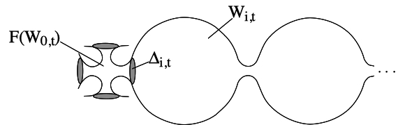
Figure 2. Decomposition of a 4-noid into pieces. Only one Delaunay end is represented, and $F(W_{0,t})$ is represented as an embedded domain for clarity, but in general it will be immersed.

Since $M_{0}$ is Alexandrov embedded, $N_{0}$ points to the inside in a neighborhood of each end, so $M_{t}$ has embedded ends by Proposition 5. Let $\varepsilon>0$ be the number given by our application of Theorem 6 in Section 7.2 and $f_{i,t}^{{\mathcal{D}}}:{\mathbb{C}}\setminus\{p_{i,t}\}\to{\mathbb{R}}^{3}$ be the Delaunay immersion which approximates $f_{t}$ in $D^{*}(p_{i,t},\varepsilon)$. Recall that $f_{t}(D^{*}(p_{i,t},\varepsilon))$ is embedded. Let $\widetilde{f}_{t}=\frac{1}{t}f_{t}$. By Proposition 4, $\widetilde{f}_{t}$ converges to $\psi$ on compact subsets of $\Sigma_{0}$, where $\psi:\Sigma_{0}\to{\mathbb{R}}^{3}$ is a parametrization of $M_{0}$. Since $M_{0}$ has catenoidal ends, we may assume (taking $\varepsilon$ smaller if necessary) that $\psi(D^{*}(p_{i,0},\varepsilon))$ is embedded and $N_{0}\neq N_{0}(p_{i,0})$ in $D^{*}(p_{i,0},\varepsilon)$.

Let $h_{i}:{\mathbb{R}}^{3}\to{\mathbb{R}}$ be the height function in the direction $N_{0}(p_{i,0})$, defined by

$$h_{i}(x)=\langle x,N_{0}(p_{i,0})\rangle.$$

We shall cut $M_{t}$ by the plane $h_{i}=\delta$ where $\delta>0$ is a fixed, large enough number such that for $1\leq i\leq n$,

$$\delta>\max_{C(p_{i,0},\varepsilon)}h_{i}\circ\psi.$$

Since $\displaystyle\lim_{z\to p_{i,0}}h_{i}\circ\psi(z)=+\infty$, we may fix a positive, small enough $\varepsilon^{\prime}<\varepsilon$ such that

$$\min_{C(p_{i,0},\varepsilon^{\prime})}h_{i}\circ\psi>\delta.$$

Let ${\mathcal{A}}_{i,t}$ be the annulus defined by $\varepsilon^{\prime}\leq|z-p_{i,t}|\leq\varepsilon$. Since $N_{0}\neq N_{0}(p_{i,0})$ in ${\mathcal{A}}_{i,0}$,

$$\min_{{\mathcal{A}}_{i,0}}\|N_{0}(z)-N_{0}(p_{i,0})\|>0.$$

For $t>0$ small enough:

(24) $$\max_{C(p_{i,t},\varepsilon)}h_{i}\circ\widetilde{f}_{t}<\delta$$

(25) $$\min_{C(p_{i,t},\varepsilon^{\prime})}h_{i}\circ\widetilde{f}_{t}>\delta$$

(26) $$\min_{{\mathcal{A}}_{i,t}}\|N_{t}(z)-N_{0}(p_{i,0})\|>0.$$

Hence the function $h_{i}\circ\widetilde{f}_{t}$ has no critical point in the annulus ${\mathcal{A}}_{i,t}$. So $h_{i}\circ\widetilde{f}_{t}=\delta$ defines a regular closed curve $\gamma_{i,t}$ in ${\mathcal{A}}_{i,t}$. At $t=0$, $h_{i}\circ\psi=\delta$ is a single curve around $p_{i,0}$, so $\gamma_{i,t}$ has only one component and is not contractible in ${\mathcal{A}}_{i,t}$. Let $D_{i,t}\subset{\mathbb{C}}$ be the topological disk bounded by $\gamma_{i,t}$ and $D_{i,t}^{*}=D_{i,t}\setminus\{p_{i,t}\}$. Let $\Delta_{i,t}$ be the closed topological disk bounded by $\widetilde{f}_{t}(\gamma_{i,t})$ in the plane defined by $h_{i}(x)=\delta$.

Claim 2.

For $t>0$ small enough, $\widetilde{f}_{t}(D_{i,t}^{*})\cap\Delta_{i,t}=\emptyset$.

Proof: of course, $h_{i}\circ\widetilde{f}_{t}>\delta$ in $D_{i,t}^{*}\cap{\mathcal{A}}_{i,t}$. What we need to prove is that $\widetilde{f}_{t}(D^{*}(p_{i,t},\varepsilon^{\prime}))$ does not intersect $\Delta_{i,t}$. We do this by comparison with the Delaunay surface. Let $\Pi_{i}=N_{0}(p_{i,0})^{\perp}$ and $\pi_{i}={\mathbb{R}}^{3}\to\Pi_{i}$ be the orthogonal projection. Since $\psi$ has a catenoidal end at $p_{i,0}$, $\psi({\mathcal{A}}_{i,t})$ is a graph over an annulus in the plane $\Pi_{i}$, with inside boundary circle $\pi_{i}\circ\psi(C(p_{i,t},\varepsilon))$ and outside boundary circle $\pi_{i}\circ\psi(C(p_{i,t},\varepsilon^{\prime}))$. Moreover, $N_{0}$ is close to $N_{0}(p_{i,t})$. Since $\widetilde{f}_{t}$ is $C^{1}$ close to $\psi$ in ${\mathcal{A}}_{i,t}$, for $t>0$ small enough, $\widetilde{f}_{t}({\mathcal{A}}_{i,t})$ is a graph over an annulus in the plane $\Pi_{i}$, with inside boundary circle $\pi_{i}\circ\widetilde{f}_{t}(C(p_{i,t},\varepsilon))$ and outside boundary circle $\pi_{i}\circ\widetilde{f}_{t}(C(p_{i,t},\varepsilon^{\prime}))$.

Now we go back to the original scale. Since $f_{t}$ is $C^{1}$ close to $f_{i,t}^{{\mathcal{D}}}$ in $D^{*}(p_{i,t},\varepsilon)$, we conclude that $f_{i,t}^{{\mathcal{D}}}({\mathcal{A}}_{i,t})$ is a graph over an annulus in the plane $\Pi_{i}$, with inside boundary circle $\pi_{i}\circ f_{i,t}^{{\mathcal{D}}}(C(p_{i,t},\varepsilon))$ and outside boundary circle $\pi_{i}\circ f_{i,t}^{{\mathcal{D}}}(C(p_{i,t},\varepsilon^{\prime}))$. Then from the geometry of Delaunay surfaces, there exists a curve $\gamma_{i,t,0}$ in $D^{*}(p_{i,t},\varepsilon^{\prime})$ such that $f_{i,t}^{{\mathcal{D}}}(\gamma_{i,t,0})$ is a closed curve in the plane $h_{i}=\frac{1}{2}$. Let $D_{i,t,0}$ be the disk bounded by $\gamma_{i,t,0}$ and ${\mathcal{A}}_{i,t,0}$ be the closed annulus bounded by $\gamma_{i,t}$ and $\gamma_{i,t,0}$. Then $h_{i}\circ f_{i,t}^{{\mathcal{D}}}>\frac{1}{2}$ in $D_{i,t,0}$ and $f_{i,t}^{{\mathcal{D}}}({\mathcal{A}}_{i,t,0})$ is a graph over an annulus in the plane $\Pi_{i}$. Since $f_{t}$ is $C^{1}$ close to $f_{i,t}^{{\mathcal{D}}}$ in $D^{*}(p_{i,t},\varepsilon)$, we conclude that $h_{i}\circ f_{t}>\frac{1}{4}$ in $D_{i,t,0}^{*}$ and $f_{t}({\mathcal{A}}_{i,t,0})$ is a graph over an annulus in the plane $\Pi_{i}$.

Back to the scale $\frac{1}{t}$, $\widetilde{f}_{t}(D_{i,t}\cap{\mathcal{A}}_{i,t,0})$ is a graph over an annulus in the plane $\Pi_{i}$ whose inside boundary circle is $\pi_{i}\circ\widetilde{f}_{t}(\gamma_{i,t})=\pi_{i}(\partial\Delta_{i,t})$, so $\widetilde{f}_{t}(D_{i,t}\cap{\mathcal{A}}_{i,t,0})\cap\Delta_{i,t}=\emptyset$. Moreover, $h_{i}\circ\widetilde{f}_{t}>\frac{1}{4t}\gg\delta$ in $D_{i,t,0}^{*}$ so $\widetilde{f}_{t}(D^{*}_{i,t,0})\cap\Delta_{i,t}=\emptyset$. $\Box$

Claim 3.

For $t>0$ small enough, $\widetilde{f}_{t}(D_{i,t}^{*})\cup\Delta_{i,t}$ is the boundary of a cylindrically bounded domain $W_{i,t}\subset{\mathbb{R}}^{3}$.

Proof: since $f_{t}$ is close to $f_{i,t}^{{\mathcal{D}}}$ in $D_{i,t}^{*}$, we can find an increasing diverging sequence $(R_{t,k})_{k\in{\mathbb{N}}}$ such that $f_{t}(D_{i,t}^{*})$ intersects the plane $h_{i}=R_{t,k}$ transversally along a closed curve $f_{t}(\gamma_{i,t,k})$. (Explicitely, we can take $R_{t,k}=\frac{1}{2}+k\,h_{i}(T_{t})$ where $T_{t}\in{\mathbb{R}}^{3}$ is the period of the Delaunay surface $f_{i,t}^{{\mathcal{D}}}$.) Let ${\mathcal{A}}_{i,t,k}$ be the annulus bounded by $\gamma_{i,t}$ and $\gamma_{i,t,k}$. Let $\Delta_{i,t,k}$ be the closed disk bounded by $\widetilde{f}_{t}(\gamma_{i,t,k})$ in the plane $h_{i}=t^{-1}R_{t,k}$. Then $\widetilde{f}_{t}({\mathcal{A}}_{i,t,k})\cup\Delta_{i,t}\cup\Delta_{i,t,k}$ is topologically a sphere: the image of ${\mathbb{S}}^{2}$ by an injective continuous map. By the Jordan Brouwer Theorem, it is the boundary of a bounded domain $W_{i,t,k}$. Clearly, $W_{i,t,k}\subset W_{i,t,k+1}$. We take $W_{i,t}=\bigcup_{k\in{\mathbb{N}}}W_{i,t,k}$. $\Box$

Let $\Omega_{t}={\mathbb{C}}\cup\{\infty\}\setminus(D_{1,t}\cup\cdots\cup D_{n,t})$. Let $W^{\prime}$ be the flat 3-manifold given by Lemma 1 and denote $F:W^{\prime}\to{\mathbb{R}}^{3}$ its developing map (instead of $F^{\prime}$). (Here $W^{\prime}$ is an open manifold, meaning not a manifold-with-boundary.)

Claim 4.

For $t>0$ small enough, there exists a compact domain $W_{0,t}$ in $W^{\prime}$ such that

$$F(\partial W_{0,t})=\widetilde{f}_{t}(\Omega_{t})\cup\Delta_{1,t}\cup\cdots\cup\Delta_{n,t}.$$

Proof: by definition, $\psi$ lifts to a diffeomorphism $\widehat{\psi}:\Sigma_{0}\to S\subset W^{\prime}$ such that $F\circ\widehat{\psi}=\psi$. Since $M_{0}$ has catenoidal ends, there exists domains $V_{1},\cdots,V_{n}$ in $W^{\prime}$ such that for $1\leq i\leq n$:

• $F:V_{i}\to F(V_{i})\subset{\mathbb{R}}^{3}$ is a diffeomorphism,

• $V_{i}$ is foliated by flat disks on which $h_{i}\circ F$ is constant (in particular, $h_{i}\circ F$ is constant on $\partial V_{i}$),

• $\widehat{\psi}(D^{*}(p_{i,0},\varepsilon))\subset V_{i}$ (which might require taking a smaller $\varepsilon>0$),

• $h_{i}<\delta$ on $V_{i}\cap\widehat{\psi}(\Sigma_{0}\setminus\bigcup_{i=1}^{n}D(p_{i,0},\varepsilon))$ (which might require taking a larger $\delta$).

Let $r>0$ be the radius of the embedded tubular neighborhood of $S$ in $W^{\prime}$ constructed in Lemma 1. For $t>0$ small enough, $||\widetilde{f}_{t}-\psi||<r$ in $\overline{\Omega}_{t}$, so $\widetilde{f}_{t}$ lifts to $\widehat{f}_{t}:\overline{\Omega}_{t}\to W^{\prime}$ such that $F\circ\widehat{f}_{t}=\widetilde{f}_{t}$. (Explicitely, $\widehat{f}_{t}(z)=\exp_{\psi(z)}(\widetilde{f}_{t}(z)-\psi(z)).$) From the properties of $V_{i}$ and the convergence of $\widehat{f}_{t}$ to $\widehat{\psi}$ on compact subsets of $\Sigma_{0}$, we have for $t>0$ small enough

(27) $$\widehat{f}_{t}(\overline{\Omega}_{t}\cap D(p_{i,0},\varepsilon))\subset V_{i}$$

(28) $$h_{i}<\delta\quad\mbox{ on $V_{i}\cap\widehat{f}_{t}(\Sigma_{0}\setminus\bigcup_{i=1}^{n}D(p_{i,0},\varepsilon))$}.$$

By Equation (27), $\widehat{f}_{t}(\gamma_{i,t})\subset V_{i}$ so $\Delta_{i,t}$ lifts to a closed disk $\widehat{\Delta}_{i,t}\subset V_{i}$ such that $\partial\widehat{\Delta}_{i,t}=\widehat{f}_{t}(\gamma_{i,t})$ and $F(\widehat{\Delta}_{i,t})=\Delta_{i,t}$. Since $F$ is a diffeomorphism on $V_{i}$, $\widehat{f}_{t}(\Omega_{t}\cap D(p_{i,t},\varepsilon))$ is disjoint from $\widehat{\Delta}_{i,t}$. By (28), $\widehat{f}_{t}(\Omega_{t}\setminus\bigcup_{i=1}^{n}D(p_{i,t},\varepsilon))$ is disjoint from $\widehat{\Delta}_{i,t}$. Hence $\widehat{f}_{t}(\Omega_{t})\cap\widehat{\Delta}_{i,t}=\emptyset$. Then $\widehat{f}_{t}(\Omega_{t})\cup\widehat{\Delta}_{1,t}\cup\cdots\cup\widehat{\Delta}_{n,t}$ is a topological sphere in $W^{\prime}$. Since $M_{0}$ has genus zero, $W^{\prime}$ is homeomorphic to ${\mathbb{R}}^{3}$. By the Jordan Brouwer Theorem, $\widehat{f}_{t}(\Omega_{t})\cup\widehat{\Delta}_{1,t}\cup\cdots\cup\widehat{\Delta}_{n,t}$ is the boundary of a compact domain $W_{0,t}\subset W^{\prime}$. $\Box$

Returning to the proof of Proposition 6, let $W_{t}$ be the abstract 3-manifold with boundary obtained as the disjoint union $\overline{W}_{0,t}\sqcup\overline{W}_{1,t}\sqcup\cdots\sqcup\overline{W}_{n,t}$, identifying $\overline{W}_{0,t}$ and $\overline{W}_{i,t}$ along their boundaries $\widehat{\Delta}_{i,t}$ and $\Delta_{i,t}$ via the map $F$ for $1\leq i\leq n$. Let $F_{t}:W_{t}\to{\mathbb{R}}^{3}$ be the map defined by $F_{t}=F$ in $\overline{W}_{0,t}$ and $F_{t}=\mbox{id}$ in $\overline{W}_{i,t}$ for $1\leq i\leq n$. Then $F_{t}$ is a proper local diffeomorphism whose boundary restriction parametrizes $M_{t}$. Moreover, since each $\overline{W}_{i,t}$ is homeomorphic to a closed ball minus a boundary point, we may compactify $W_{t}$ by adding $n$ points. This proves that $M_{t}$ is Alexandrov-embedded. $\Box$

Appendix A Appendix: complements on the Banach algebra ${\mathcal{W}}_{\rho}$

In this section, we prove several basic facts about the Banach algebra ${\mathcal{W}}_{\rho}$ introduced in Section 3.6 that are used in this paper and related papers [14, 15].

Proposition 7.

If $\rho\geq 1$, ${\mathcal{W}}_{\rho}$ is a Banach algebra.

Proof: let $f,g\in{\mathcal{W}}_{\rho}$ and $h=fg$. Then $(|f_{i}|\rho^{|i|})_{i\in{\mathbb{Z}}}$ and $(|g_{i}|\rho^{|i|})_{i\in{\mathbb{Z}}}$ are summable families, so $(|f_{i}g_{j}|\rho^{|i|+|j|})_{(i,j)\in{\mathbb{Z}}^{2}}$ is a summable family. Using the triangular inequality and $\rho\geq 1$, we obtain that $|f_{i}g_{j}|\rho^{|i+j|}$ is a summable family, so the following computation is valid:

$$\sum_{i\in{\mathbb{Z}}}|h_{i}|\rho^{|i|}\leq\sum_{(i,k)\in{\mathbb{Z}}^{2}}|f_{k}g_{i-k}|\rho^{|i|}=\sum_{(i,j)\in{\mathbb{Z}}^{2}}|f_{i}g_{j}|\rho^{|i+j|}\leq\sum_{i\in{\mathbb{Z}}}|f_{i}|\rho^{|i|}\sum_{j\in{\mathbb{Z}}}|g_{j}|\rho^{|j|}.$$

Hence $h\in{\mathcal{W}}_{\rho}$ and $\|h\|\leq\|f\|\times\|g\|$. $\Box$

Recall that if $L$ is a loop group, $L_{\rho}\subset L$ denotes the subgroup of loops whose entries are in the Banach algebra ${\mathcal{W}}_{\rho}$.

Proposition 8.

Let $\Phi\in\Lambda SL(2,{\mathbb{C}})_{\rho}$ and $(F,B)$ be its Iwasawa decomposition. Then $F\in\Lambda SU(2)_{\rho}$ and $B\in\Lambda_{+}^{{\mathbb{R}}}SL(2,{\mathbb{C}})_{\rho}$.

Proof: $\Phi$ extends holomorphically to the annulus $\frac{1}{\rho}<|\lambda|<\rho$ and $B$ extends holomorphically to the disk $|\lambda|<1$, so $F=\Phi B^{-1}$ extends holomorphically to the annulus $\frac{1}{\rho}<|\lambda|<1$. By an application of the Schwarz reflection principle, the fact that $F(\lambda)\in SU(2)$ on the unit circle implies that $F$ extends holomorphically to the annulus $\frac{1}{\rho}<|\lambda|<\rho$ and satisfies (see details in Appendix A of [11]):

$$F_{11}(\mbox{$\frac{1}{\overline{\lambda}}$})=\overline{F_{22}(\lambda)}\quad\mbox{ and }\quad F_{12}(\mbox{$\frac{1}{\overline{\lambda}}$})=-\overline{F_{21}(\lambda)}.$$

We expand $F=(F_{k\ell})_{1\leq k,\ell\leq 2}$ in the annulus $\frac{1}{\rho}<|\lambda|<\rho$ as

$$F(\lambda)=\sum_{i\in{\mathbb{Z}}}F_{i}\lambda^{i}\quad\mbox{ with }\quad F_{i}=(F_{k\ell,i})_{1\leq k,\ell\leq 2}.$$

Then for all $i\in{\mathbb{Z}}$

(29) $$F_{11,-i}=\overline{F_{22,i}}\quad\mbox{ and }\quad F_{12,-i}=-\overline{F_{21,i}}.$$

We expand $\Phi$ and $B^{-1}$ in the annulus $\frac{1}{\rho}<|\lambda|<1$ as

$$\Phi(\lambda)=\sum_{i\in{\mathbb{Z}}}\Phi_{i}\lambda^{i},\qquad B^{-1}(\lambda)=\sum_{i\in{\mathbb{Z}}}C_{i}\lambda^{i}$$

with $C_{i}=0$ for $i<0$. Then

$$F_{i}=\sum_{j\in{\mathbb{Z}}}\Phi_{j}C_{i-j}.$$

Since $\Phi\in\Lambda SL(2,{\mathbb{C}})_{\rho}$, $(\|\Phi_{i}\|\rho^{-i})_{i\in{\mathbb{Z}}}$ is a summable family (here $\|A\|=\max|A_{k\ell}|$ for $A\in{\mathcal{M}}_{2}({\mathbb{C}})$). Since $B^{-1}$ is holomorphic in the unit disk, $(\|C_{i}\|\rho^{-i})_{i\in{\mathbb{Z}}}$ is a summable family. Hence

$$\sum_{i\in{\mathbb{Z}}}\|F_{i}\|\rho^{-i}<\infty.$$

By Equation (29), this implies

$$\sum_{i\in{\mathbb{Z}}}\|F_{i}\|\rho^{i}<\infty.$$

Hence $F\in{\mathcal{M}}_{2}({\mathcal{W}}_{\rho})$. Since ${\mathcal{W}}_{\rho}$ is a Banach algebra, $B=F^{-1}\Phi\in{\mathcal{M}}_{2}({\mathcal{W}}_{\rho})$ as well. $\Box$

Remark 4.

If $\Phi\in\Lambda SL(2,{\mathbb{C}})$ is a Laurent polynomial of degree $d$, a similar argument proves that $F$ is a Laurent polynomial of degree at most $d$ and $B$ is a polynomial of degree at most $2d$.

The loop groups $\Lambda SL(2,{\mathbb{C}})_{\rho}$, $\Lambda SU(2)_{\rho}$ and $\Lambda_{+}^{{\mathbb{R}}}SL(2,{\mathbb{C}})_{\rho}$ are Banach manifolds. This can be proved using the submersion criterion (see [1], 5.9.1 for the definition of a submersion in the Banach case). The tangent space at $I_{2}$ of these Banach Lie groups are respectively the following Banach Lie algebras:

$$\Lambda\mathfrak{sl}(2,{\mathbb{C}})_{\rho}=\{M\in{\mathcal{M}}_{2}({\mathcal{W}}_{\rho}):M_{11}+M_{22}=0\}$$

$$\Lambda\mathfrak{su}(2)_{\rho}=\{M\in{\mathcal{M}}_{2}({\mathcal{W}}_{\rho}):M_{11}+M_{22}=0,\;M_{11}+M_{11}^{*}=0,\;M_{12}+M_{21}^{*}=0\}$$

$$\Lambda_{+}^{{\mathbb{R}}}\mathfrak{sl}(2,{\mathbb{C}})_{\rho}=\{M\in{\mathcal{M}}_{2}({\mathcal{W}}_{\rho}^{\geq 0}):M_{11}+M_{22}=0,\;M_{11}(0)\in{\mathbb{R}},\;M_{21}(0)=0\}.$$

Proposition 9.

$$\Lambda\mathfrak{sl}(2,{\mathbb{C}})_{\rho}=\Lambda\mathfrak{su}(2)_{\rho}\oplus\Lambda_{+}^{{\mathbb{R}}}\mathfrak{sl}(2,{\mathbb{C}})_{\rho}.$$

Proof:

• Let $M\in\Lambda\mathfrak{su}(2)_{\rho}\cap\Lambda_{+}^{{\mathbb{R}}}\mathfrak{sl}(2,{\mathbb{C}})_{\rho}$. Then all entries of $M$ are in ${\mathcal{W}}_{\rho}^{\geq 0}\cap{\mathcal{W}}_{\rho}^{\leq 0}={\mathcal{W}}^{0}$ so $M$ is constant. It is then straightforward that $M=0$.

• Let $M\in\Lambda\mathfrak{sl}(2,{\mathbb{C}})_{\rho}$ and write

  $$M(\lambda)=\sum_{n\in{\mathbb{Z}}}M_{n}\lambda^{n}\quad\mbox{ with }\quad M_{0}=\left(\begin{array}[]{cc}a_{0}&b_{0}\\ c_{0}&-a_{0}\end{array}\right).$$

  Define

  $$\mbox{\rm uni}(M)(\lambda)=\left(\begin{array}[]{cc}{\rm i}\,{\rm Im}(a_{0})&-\overline{c_{0}}\\ c_{0}&-{\rm i}\,{\rm Im}(a_{0})\end{array}\right)+\sum_{n<0}\left(M_{n}\lambda^{n}-\mbox{}^{t}\overline{M}_{n}\lambda^{-n}\right)\in\Lambda\mathfrak{su}(2)_{\rho}$$

  $$\mbox{\rm pos}(M)(\lambda)=\left(\begin{array}[]{cc}{\rm Re}(a_{0})&b_{0}+\overline{c_{0}}\\ 0&-{\rm Re}(a_{0})\end{array}\right)+\sum_{n>0}M_{n}\lambda^{n}+\sum_{n<0}\mbox{}^{t}\overline{M}_{n}\lambda^{-n}\in\Lambda_{+}^{{\mathbb{R}}}\mathfrak{sl}(2,{\mathbb{C}})_{\rho}.$$

  Then $M=\mbox{\rm uni}(M)+\mbox{\rm pos}(M)$. $\Box$

Theorem 5.

Iwasawa decomposition is a smooth diffeomorphism (in the sense of Banach manifolds) from $\Lambda SL(2,{\mathbb{C}})_{\rho}$ to $\Lambda SU(2)_{\rho}\times\Lambda_{+}^{{\mathbb{R}}}SL(2,{\mathbb{C}})_{\rho}$. Moreover, its differential at $I_{2}$ is given by $d\mbox{\rm Uni}(I_{2})=\mbox{\rm uni}$ and $d\mbox{\rm Pos}(I_{2})=\mbox{\rm pos}$.

Proof: consider the following smooth map:

$$p:\Lambda SU(2)_{\rho}\times\Lambda_{+}^{{\mathbb{R}}}SL(2,{\mathbb{C}})_{\rho}\to\Lambda SL(2,{\mathbb{C}})_{\rho},\quad p(F,B)=FB.$$

Then

$$dp(I_{2},I_{2}):\Lambda\mathfrak{su}(2)_{\rho}\times\Lambda_{+}^{{\mathbb{R}}}\mathfrak{sl}(2,{\mathbb{C}})_{\rho}\to\Lambda\mathfrak{sl}(2,{\mathbb{C}})_{\rho},\quad dp(I_{2},I_{2})(F,B)=F+B.$$

By Proposition 9, $dp(I_{2},I_{2})$ is an isomorphism. By the Inverse Mapping Theorem, $p$ is a local diffeomorphism in a neighborhood of $(I_{2},I_{2})$. Let $(F_{0},B_{0})\in\Lambda SU(2)_{\rho}\times\Lambda_{+}^{{\mathbb{R}}}SL(2,{\mathbb{C}})_{\rho}$. Consider the maps

$$f_{1}:\Lambda SU(2)_{\rho}\times\Lambda_{+}^{{\mathbb{R}}}SL(2,{\mathbb{C}})_{\rho}\to\Lambda SU(2)_{\rho}\times\Lambda_{+}^{{\mathbb{R}}}SL(2,{\mathbb{C}})_{\rho},\quad f_{1}(F,B)=(F_{0}F,BB_{0})$$

$$f_{2}:\Lambda SL(2,{\mathbb{C}})_{\rho}\to\Lambda SL(2,{\mathbb{C}})_{\rho},\quad f_{2}(\Phi)=F_{0}\Phi B_{0}.$$

Then $f_{1}$ is a diffeomorphism with inverse $(F,B)\mapsto(F_{0}^{-1}F,BB_{0}^{-1})$ and $f_{2}$ is a diffeomorphism with inverse $\Phi\mapsto F_{0}^{-1}\Phi B_{0}^{-1}$. We have

$$f_{2}\circ p\circ f_{1}^{-1}=p$$

so $p$ is a local diffeomorphism in a neighborhood of any $(F_{0},B_{0})$. Since $p$ is injective (by the standard Iwasawa decomposition theorem) and onto (by Proposition 8), $p$ is a smooth diffeomorphism. Iwasawa decomposition is of course the inverse of $p$. $\Box$

As an application of Theorem 5, let us prove Equation (8) by differentiation of the Sym-Bobenko formula (6). In the following computation, we omit the $\lambda$ variable. Fix $z_{0}\in\Sigma$ and define $\widetilde{\Phi}(z)=F(z_{0})^{-1}\Phi(z)B(z_{0})^{-1}$. Then

$$d\widetilde{\Phi}(z_{0})=F(z_{0})^{-1}\Phi(z_{0})\xi(z_{0})B(z_{0})^{-1}=B(z_{0})\xi(z_{0})B(z_{0})^{-1}.$$

Writing $B(z_{0})^{0}=\left(\begin{smallmatrix}\rho&\mu\\ 0&\rho^{-1}\end{smallmatrix}\right)$ and $\xi_{12}(z_{0})=\lambda^{-1}\beta$, we have

$$d\widetilde{\Phi}(z_{0})^{-}=\left(\begin{array}[]{cc}\rho&\mu\\ 0&\rho^{-1}\end{array}\right)\left(\begin{array}[]{cc}0&\lambda^{-1}\beta^{0}\\ 0&0\end{array}\right)\left(\begin{array}[]{cc}\rho^{-1}&-\mu\\ 0&\rho\end{array}\right)=\left(\begin{array}[]{cc}0&\rho^{2}\lambda^{-1}\beta^{0}\\ 0&0\end{array}\right).$$

Since $\widetilde{\Phi}(z_{0})=I_{2}$, Theorem 5 yields

$$F(z_{0})^{-1}dF(z_{0})=d\widetilde{F}(z_{0})=\mbox{\rm uni}(d\widetilde{\Phi}(z_{0}))=\left(\begin{array}[]{cc}0&\rho^{2}\lambda^{-1}\beta^{0}\\ -\rho^{2}\lambda\overline{\beta^{0}}&0\end{array}\right)+\mbox{constant}$$

$$\frac{\partial}{\partial\lambda}\left(F(z_{0})^{-1}dF(z_{0})\right)|_{\lambda=1}=\left(\begin{array}[]{cc}0&-\rho^{2}\beta^{0}\\ -\rho^{2}\overline{\beta^{0}}&0\end{array}\right).$$

By differentiation of the Sym-Bobenko formula, we obtain (omitting $z_{0}$)

$$df = -2{\rm i}\left(\frac{\partial dF}{\partial\lambda}F^{-1}-\frac{\partial F}{\partial\lambda}F^{-1}dFF^{-1}\right)|_{\lambda=1}$$

$$= -2{\rm i}F\frac{\partial}{\partial\lambda}\left(F^{-1}dF\right)F^{-1}|_{\lambda=1}$$

$$= 2{\rm i}\rho^{2}F\left(\begin{array}[]{cc}0&\beta^{0}\\ \overline{\beta^{0}}&0\end{array}\right)F^{-1}|_{\lambda=1}.$$

Appendix B Appendix: On Delaunay ends in the DPW method

We consider the standard Delaunay residue for $t\leq\frac{1}{16}$:

$$A_{t}(\lambda)=\left(\begin{array}[]{cc}0&\lambda^{-1}r+s\\ \lambda r+s&0\end{array}\right)\qquad\mbox{ where }\left\{\begin{array}[]{l}r+s=\frac{1}{2}\\ rs=t\\ r<s\end{array}\right.$$

In particular, in the limit case $t=0$, we have

$$A_{0}=\left(\begin{array}[]{cc}0&\frac{1}{2}\\ \frac{1}{2}&0\end{array}\right).$$

Let ${\mathbb{A}}_{\rho}$ be the annulus $\frac{1}{\rho}<|\lambda|<\rho$, where $\rho>1$.

Definition 6 ([11]).

A perturbed Delaunay potential is a family of DPW potentials $\xi_{t}$ of the form

$$\xi_{t}(z,\lambda)=A_{t}(\lambda)\frac{dz}{z}+R_{t}(z,\lambda)dz$$

where $R_{t}$ is of class $C^{2}$ with respect to $(t,z,\lambda)\in(-T,T)\times D(0,\varepsilon)\times{\mathbb{A}}_{\rho}$ for some positive $\varepsilon$ and $T$, and satisfies $R_{0}=0$. In particular, $\xi_{0}=A_{0}\frac{dz}{z}$.

Let $(e_{1},e_{2},e_{3})$ represent the canonical basis of ${\mathbb{R}}^{3}$ in the $\mathfrak{su}(2)$ model.

Theorem 6.

Let $\xi_{t}$ be a perturbed Delaunay potential. Let $\Phi_{t}(z,\lambda)$ be a family of solutions of $d\Phi_{t}=\Phi_{t}\xi_{t}$ in the universal cover of the punctured disk $D^{*}(0,\varepsilon)$. Assume that $\Phi_{t}(z,\lambda)$ depends continuously on $(t,z,\lambda)$ and that the Monodromy Problem for $\Phi_{t}$ is solved. Let $f_{t}=\mbox{\rm Sym}(\mbox{\rm Uni}(\Phi_{t}))$ be the immersion given by the DPW method. Finally, assume that $\Phi_{0}(1,\cdot)$ is constant (i.e. independent of $\lambda$).

Given $0<\alpha<1$, there exists uniform positive numbers $\varepsilon^{\prime}\leq\varepsilon$, $T^{\prime}\leq T$, $c$ and a family of Delaunay immersions $f_{t}^{{\mathcal{D}}}:{\mathbb{C}}^{*}\to{\mathbb{R}}^{3}$ such that:

1. For $0<|t|<T^{\prime}$ and $0<|z|<\varepsilon^{\prime}$:

   $$\|f_{t}(z)-f_{t}^{{\mathcal{D}}}(z)\|\leq c|t|\,|z|^{\alpha}.$$

2. For $0<t<T^{\prime}$, $f_{t}:D^{*}(0,\varepsilon^{\prime})\to{\mathbb{R}}^{3}$ is an embedding.

3. The end of $f_{t}^{{\mathcal{D}}}$ at $z=0$ has weight $8\pi t$ and its axis converges when $t\to 0$ to the half-line spanned by the vector $Qe_{3}Q^{-1}$ where

   $$Q=\mbox{\rm Uni}\left(\Phi_{0}(1)H\right)\quad\mbox{ and }\quad H=\frac{1}{\sqrt{2}}\left(\begin{array}[]{cc}1&1\\ -1&1\end{array}\right).$$

Thomas Raujouan has proved this result in [11], Theorem 3, in the case $\Phi_{0}(1,\lambda)=I_{2}$. He proves that the limit axis is spanned by $e_{1}$. (In fact, he finds that the limit axis is $-e_{1}$, but this is because he has the opposite sign in the Sym-Bobenko formula. See Remark 2.) Then in Section 2 of [11], he explains, in the case $r>s$, how to extend his result to the case where $\Phi_{0}(1,\lambda)$ is constant. We adapt his method to the case $r<s$.

Lemma 2.

There exists a gauge $G(z)$ and a change of variable $h(z)$ with $h(0)=0$ such that $\widetilde{\xi}_{t}=(h^{*}\xi_{t})\cdot G$ is a perturbed Delaunay potential (with residue $A_{t}$) and $\widetilde{\Phi}_{t}=(h^{*}\Phi_{t})\times G$ satisfies at $t=0$

(31) $$\widetilde{\Phi}_{0}(1,\lambda)=QH^{-1}\in\Lambda SU(2).$$

Proof: we follow the method explained in Section 2 of [11]. We take the change of variable in the form

$$h(z)=\frac{z}{pz+q}$$

where $p,q$ are complex numbers (independent of $t$) to be determined, with $q\neq 0$. We consider the following gauge:

$$G(z)=\frac{1}{\sqrt{q(pz+q)}}\left(\begin{array}[]{cc}pz+q&pz\\ 0&q\end{array}\right).$$

It is chosen so that

(32) $$G(0)=I_{2}\quad\mbox{ and }\quad dG=GA_{0}\frac{dz}{z}-A_{0}G\frac{dh}{h}.$$

(In fact, the gauge $G$ is found as the only solution of Problem (32) which is upper triangular.) We have

$$\widetilde{\xi}_{t}=(h^{*}\xi_{t})\cdot G=G^{-1}\left(A_{t}(\lambda)\frac{dh}{h}+R_{t}(h,\lambda)dh\right)G+G^{-1}dG.$$

Since $G(0)=I_{2}$, $\widetilde{\xi}_{t}$ has a simple pole at $z=0$ with residue $A_{t}$. Using Equation (32), we obtain at $t=0$:

$$\widetilde{\xi}_{0}=G^{-1}A_{0}\frac{dh}{h}G+G^{-1}dG=A_{0}\frac{dz}{z}.$$

Hence $\widetilde{\xi}_{t}$ is a perturbed Delaunay potential. It remains to compute $\widetilde{\Phi}_{0}(1)$. The matrix $H$ diagonalises $A_{0}$:

$$A_{0}=H\left(\begin{array}[]{cc}\frac{-1}{2}&0\\ 0&\frac{1}{2}\end{array}\right)H^{-1}$$

Hence

$$\Phi_{0}(z)=\Phi_{0}(1)z^{A_{0}}=\Phi_{0}(1)H\left(\begin{array}[]{cc}\frac{1}{\sqrt{z}}&0\\ 0&\sqrt{z}\end{array}\right)H^{-1}$$

$$\widetilde{\Phi}_{0}(1) = \Phi_{0}(h(1))G(1)$$

$$= \Phi_{0}(1)H\left(\begin{array}[]{cc}\sqrt{p+q}&0\\ 0&\frac{1}{\sqrt{p+q}}\end{array}\right)H^{-1}\frac{1}{\sqrt{q(p+q)}}\left(\begin{array}[]{cc}p+q&p\\ 0&q\end{array}\right)$$

$$= \Phi_{0}(1)H\left(\begin{array}[]{cc}\sqrt{q}&\frac{p}{\sqrt{q}}\\ 0&\frac{1}{\sqrt{q}}\end{array}\right)H^{-1}$$

We decompose $\Phi_{0}(1)H=QR$ with $Q\in SU(2)$ and $R=\left(\begin{smallmatrix}\rho&\mu\\ 0&\frac{1}{\rho}\end{smallmatrix}\right)$. Then

$$\widetilde{\Phi}_{0}(1)=Q\left(\begin{array}[]{cc}\rho&\mu\\ 0&\frac{1}{\rho}\end{array}\right)\left(\begin{array}[]{cc}\sqrt{q}&\frac{p}{\sqrt{q}}\\ 0&\frac{1}{\sqrt{q}}\end{array}\right)H^{-1}$$

We take $q=\frac{1}{\rho^{2}}$ and $p=-\frac{\mu}{\rho}$ to cancel the two matrices in the middle and obtain Equation (31). $\Box$

We can now prove Theorem 6. Let

$$\widehat{\Phi}_{t}(z,\lambda)=HQ^{-1}\widetilde{\Phi}_{t}(z,\lambda)=HQ^{-1}\Phi_{t}(h(z),\lambda)G(z,\lambda)$$

Since $\widehat{\Phi}_{0}(1,\lambda)=I_{2}$, we can apply Theorem 3 in [11] which says that the resulting immersion $\widehat{f}_{t}$ satisfies Points 1 and 2 of Theorem 6 and its limit axis is spanned by $e_{1}$. We have

$$f_{t}\circ h=QH^{-1}\widehat{f_{t}}HQ^{-1}$$

so $f_{t}\circ h$ and $\widehat{f}_{t}$ differ by a rotation and the limit axis of $f_{t}$ is spanned by the vector $QH^{-1}e_{1}HQ^{-1}$. Now

$$H^{-1}e_{1}H=-\frac{{\rm i}}{2}\left(\begin{array}[]{cc}1&-1\\ 1&1\end{array}\right)\left(\begin{array}[]{cc}0&1\\ 1&0\end{array}\right)\left(\begin{array}[]{cc}1&1\\ -1&1\end{array}\right)=-{\rm i}\left(\begin{array}[]{cc}-1&0\\ 0&1\end{array}\right)=e_{3}.$$

$\Box$

Martin Traizet
Institut Denis Poisson
Université de Tours, 37200 Tours, France
martin.traizet@univ-tours.fr

References

- [1] N. Bourbaki: Variétés différentielles et analytiques. Eléments de mathématiques. Hermann, Paris 1971.
- [2] C. Cosín, A. Ros: A Plateau problem at infinity for properly immersed minimal surfaces with finite total curvature. Indiana Univ. Math. J. 50, no. 2 (2001), 847–879.
- [3] J. Dorfmeister, F. Pedit, H. Wu: Weierstrass type representation of harmonic maps into symmetric spaces. Communications in Analysis and Geometry 6 (1998), 633-668.
- [4] O. Forster: Lectures on Riemann surfaces. Graduate texts in Mathematics, Springer Verlag (1981).
- [5] S. Fujimori, S. Kobayashi, W. Rossman: Loop group methods for constant mean curvature surfaces. arXiv:math/0602570.
- [6] K. Große-Brauckmann, R. Kusner, J. Sullivan: Triunduloids: embedded constant mean curvature surfaces with three ends and genus zero. J. Reine Angew. Math. 564 (2003), 35–61.
- [7] K. Große-Brauckmann, R. Kusner, J. Sullivan: Coplanar constant mean curvature surfaces. Comm. Anal. Geom. 15 (2007), no. 5, 985–1023.
- [8] N. Kapouleas: Complete constant mean curvature surfaces in euclidean three-space. Annals of Mathematics 131 (1990), 239–330.
- [9] M. Kilian, W. Rossman, N. Schmitt: Delaunay ends of constant mean curvature surfaces. Compositio Mathematica 144 (2008), 186–220.
- [10] R. Mazzeo, F. Pacard: Constant mean curvature surfaces with Delaunay ends. Comm. Anal. and Geom. 9, no. 1 (2001), 169–237.
- [11] T. Raujouan: On Delaunay ends in the DPW method. To appear in Indiana Univ. Math. J. arXiv:1710.00768v2 (2017).
- [12] N. Schmitt: Constant mean curvature trinoids. arXiv:math/0403036 (2004).
- [13] N. Schmitt, M. Kilian, S. Kobayashi, W. Rossman: Unitarization of monodromy representations and constant mean curvature trinoids in 3-dimensional space forms. Journal of the London Mathematical Society 75 (2007), 563–581.
- [14] M. Traizet: Construction of constant mean curvature -noids using the DPW method. To appear in Journal für die reine und angewandte Mathematik. arXiv 1709.00924 (2017).
- [15] M. Traizet: Opening nodes in the DPW method. arXiv 1808.01366 (2018).