A Bayesian Method for Joint Clustering of Vectorial Data and Network Data

Abstract

We present a new model-based integrative method for clustering objects given both vectorial data, which describes the feature of each object, and network data, which indicates the similarity of connected objects. The proposed general model is able to cluster the two types of data simultaneously within one integrative probabilistic model, while traditional methods can only handle one data type or depend on transforming one data type to another. Bayesian inference of the clustering is conducted based on a Markov chain Monte Carlo algorithm. A special case of the general model combining the Gaussian mixture model and the stochastic block model is extensively studied. We used both synthetic data and real data to evaluate this new method and compare it with alternative methods. The results show that our simultaneous clustering method performs much better. This improvement is due to the power of the model-based probabilistic approach for efficiently integrating information.

1 Introduction

In social and economic life, as well as in many research fields such as data mining, image processing and bioinformatics, we often have the need to separate a set of objects to different groups according to their similarity to each other, so that we can subsequently represent or process different groups according to their different characteristics. As a unsupervised learning approach catering this general need, clustering data analysis has been extensively used in research and real life (Jain, 2010).

In the Big Data era, complicated systems are often measured from multiple angles. As a result, the same set of objects is often described by both their individual characteristics and their pairwise relationship. Often, the two types of data are from different sources. For example, companies, such as Amazon and Netflix, often need to divide customers into groups of different consumption patterns, so that they can correctly recommend commodities to a certain customer. In this scenario, the personal information of a customer, such as the age and historical shopping records, is the vectorial data that we can use for clustering. The interrelationship between customers, such as how often two customers shop together and how often they like same Facebook posts, is the network data that can be used for clustering. For another instance, in bioinformatics research, we often need to cluster genes into different groups, which ideally correspond to different gene regulatory modules or biochemical functions. In this scenario, the expression of genes under different conditions, such as microarray data from different tissues or different environmental stimulus, is the vectorial data for gene clustering. The network data for gene clustering includes gene regulatory networks, protein-protein interaction data and whether a pair of genes belongs to a same Gene Ontology group. Therefore, we have to integrate both vectorial data and network data to better elucidate the group structure among the objects.

Traditional clustering methods are designed for either vectorial data alone or network data alone (Buhmann, 1995). In the most commonly used vectorial data, each object is represented by a vector of the same dimension. The similarity between two objects is reflected by certain distance measure of the two corresponding vectors. The problem of clustering vectorial data have been studied for more than 60 years. The most widely used methods include K-means clustering (MacQueen, 1967; Tavazoie et al, 1999), Gaussian mixture model (McLachlan and Basford, 1988; Fraley and Raftery, 2002) and hierarchical clustering (Sibson, 1973; Defays, 1977; Eisen et al, 1998). Most vectorial data clustering methods adopted a central clustering approach by searching for a set of prototype vectors. Jain (2010) provided a good review on this subject. The other data type is network data, where the similarity between two objects is directly given without describing the characteristics of individual objects. The problem of clustering network data arose only in the recent two decades. The methods for network data clustering include entropy-based methods (Buhmann and Hofmann, 1994; Park and Pande, 2006), spectrum-based methods (Swope et al, 2004; Bowman et al, 2009), cut-based methods (Muff and Caflisch, 2009), path-based method (Jain and Stock, 2012), modified self-organizing maps (Seo and Obermayer, 2004), mean field model (Hofmann and Buhmann, 1997), probabilistic relational model (Taskar et al, 2001; Nowicki and Snijders, 2001; Mariadassou et al, 2010), and Newman’s modularity function (Newman, 2006). Fortunato (2010) provided a good review on this subject.

As shown above, vectorial data clustering and network data clustering have both been intensively studied. In contrast, as to our knowledge, no existing methods can integrate the clustering information in the two individual data types parallelly within a coherent framework. There are several papers on the direction of data integration which can take both vectorial and network data as input, but these methods either transform the network data to vectorial data as in the latent position space approach (Hoff et al, 2002; Handcock et al, 2007; Gormley and Murphy, 2011), or transform the vectorial data to network data as in Zhou et al (2010) and Gunnemann et al (2010); Günnemann et al (2011). The explicit or implicit data transformation needs an artificial design of a latent metric space for converting the network data or an artificial design of a distance measure for converting the vector data. Thus they cannot avoid the arbitrary weighting of the clustering information from two data types. In reality, we seldom know how to weight one data type again another. For example, the vectorial data and the network data may come from independent studies which may have used different techniques to check the similarity of objects at different levels. Thus, essentially we have no good way to weight one against the other. The only common and comparable thing behind the two data types is how likely each pair of objects is within a same cluster.

In this paper, we developed an integrative probabilistic clustering method called “Shared Clustering” for clustering vectorial data and network data simultaneously. We assume that the vectorial data is independent from the network data conditional on the cluster labels. Our probabilistic model treats the two types of data equally instead of treating one as the covariate of the other, and models their contribution to clustering directly instead of converting one type to another. We perform the statistical inference in the Bayesian framework. The Markov chain Monte Carlo (MCMC) algorithm, or more specifically the Gibbs sampler, is employed to sample the parameters and cluster labels. The paper is organized as follows. We first describe the model of Shared Clustering, then the inference method is described in detail, followed by applications to both synthesized data and real data. A summary and discussion are provided at the end.

2 Problem statement and model specification

We consider the clustering of $N$ objects according to their vectorial data $\mathbf{x}_{i}$ and pairwise data $\mathbf{y}_{ij}$, where $i,j=1,\ldots,N$ are the indexes of objects. Let $\boldsymbol{X}$ be the $N$-by-$q$ matrix formed by $\mathbf{x}_{i}$ whose dimension is $q$, and $\boldsymbol{Y}$ be the $N$-by-$N$ square matrix formed by $\mathbf{y}_{ij}$. Note that $\mathbf{y}_{ij}$ can be deemed as the weight of the link from the $i$-th object to the $j$-th object on the network. In the Shared Clustering model, we assume that the vectorial data $\boldsymbol{X}$ and the network data $\boldsymbol{Y}$ share a common clustering structure $\boldsymbol{C}=(c_{1},\ldots,c_{N})$, where the cluster label of the $i$-th object is $c_{i}=1,\ldots,K$, and $K$ is the total number of clusters. Given $\boldsymbol{C}$, all $\mathbf{x}_{i}$ and $\mathbf{y}_{ij}$ are assumed to be independently following their corresponding component distributions. Thus, the joint likelihood function is $L(\boldsymbol{X},\boldsymbol{Y}|\boldsymbol{\Phi},\boldsymbol{\Psi},\boldsymbol{C})=\prod\limits_{i=1}^{N}f(\mathbf{x}_{i}|\phi_{c_{i}})\cdot\prod\limits_{i=1}^{N}\prod\limits_{j=1}^{N}g(\mathbf{y}_{ij}|\psi_{c_{i},c_{j}})$, where $\boldsymbol{\Phi}=(\phi_{1},\ldots,\phi_{K})$ and $\boldsymbol{\Psi}=(\psi_{1},\ldots,\psi_{K})$ represent all component specific parameters, $f(\cdot)$ and $g(\cdot)$ represent the component distributions.

We further assume that each of the $N$ cluster labels follows a multinomial distribution with the probability vector $\boldsymbol{P}=(p_{1},\ldots,p_{K})\in\mathbbm{R}^{K}$, namely $c_{i}=k$ with probability $p_{k}$, $k=1,\ldots,K$. Intuitively, the meaning of $\boldsymbol{P}$ is the prior probabilities that each object is assigned to the corresponding clusters.

In summary, the generative version of the model can be stated as:

$$\begin{split}&c_{i}\sim\mathrm{Multinomial}(\boldsymbol{P}),\\ &\mathbf{x}_{i}|c_{i}\sim\mathrm{f}(\mathbf{x}_{i}|\phi_{c_{i}}),\\ &\mathbf{y}_{ij}|c_{i},c_{j}\sim\mathrm{g}(\mathbf{y}_{ij}|\psi_{c_{i},c_{j}}).\end{split}$$ (1)

The dependency structure of all random variables is shown in Fig. 1.

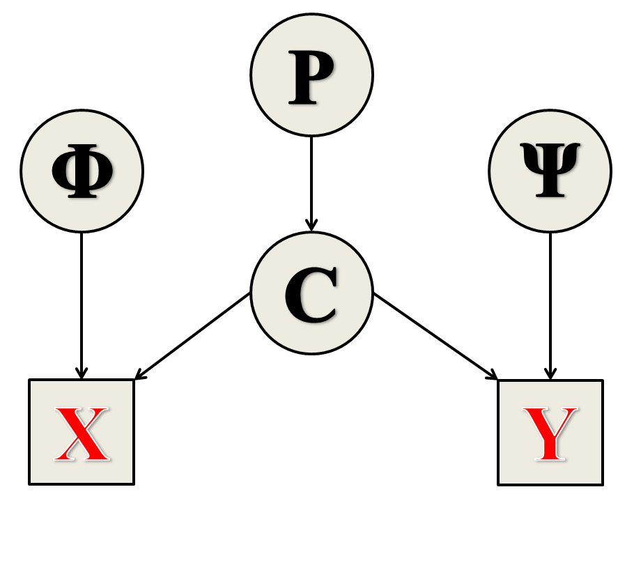
Figure 1: Dependency structure of the variables in Shared Clustering

The general joint clustering model in Equation (1) conveys the main idea to integrate the model for vectorial data and the model for network data probabilistically by conditioning on shared cluster labels, no matter what models are used for individual data types. The component distributions of $\boldsymbol{X}$ and $\boldsymbol{Y}$ can be any distribution combinations depending on the specific types of the given data. For example, $f(\cdot)$ can be either a continuous distribution or a discrete distribution depending on the given vectorial data. A proper distribution $g(\cdot)$, say Poisson distribution, may be induced to model network variables if an integer weighted graph is given.

For a concrete study of the joint clustering model, we assume that vectorial data follows a Gaussian Mixture Model (GMM) (McLachlan and Basford, 1988; Fraley and Raftery, 2002) and the network data follows a Stochastic Block Model (SBM) (Nowicki and Snijders, 2001). More specifically, we assume that the vectorial data $\mathbf{x}_{i}$ follows a multivariate Normal distribution with $\phi_{c_{i}}=(\mu_{c_{i}},\Sigma_{c_{i}})$, and $\mathbf{y}_{ij}$ is a binary variable following Bernoulli distribution with linking probability equal to $\psi_{c_{i},c_{j}}$. Here the network interested is an undirected graph without self loop, thus $\boldsymbol{Y}$ is an $N$-by-$N$ symmetric matrix with all diagonal entries being zero. In this remaining part of this paper, we will mainly focus on these two specified distribution assumptions for $\boldsymbol{X}$ and $\boldsymbol{Y}$ respectively, and we call this combination the Normal-Bernoulli model.

Under the Normal-Bernoulli model, the conditional distribution of each vector $\mathbf{x}_{i}\in\mathbbm{R}^{q},i=1,\ldots,N$ given $c_{i}$ is

$$\mathbf{x}_{i}|c_{i}\sim\mathrm{N}(\mu_{c_{i}},\Sigma_{c_{i}}),$$ (2)

where $\mu_{c_{i}}\in\mathbbm{R}^{q}$ is the mean vector and $\Sigma_{c_{i}}$ is the $q$-by-$q$ covariance matrix. From Equation (2), $\mathbf{x}_{i}$ belongs to the $k$-th cluster if and only if $c_{i}=k$, where $k=1,\ldots,K$.

In SBM, a network is partitioned into several blocks according to the number of total clusters $K$. Variables $y_{ij}$ within each individual block are controlled by a same set of parameters. In our case the parameter $\boldsymbol{\Psi}$ for network data is therefore a $K$-by-$K$ probability matrix, with each element describing the corresponding Bernoulli distribution within a certain block. Thus the distribution of the edge variable $y_{ij},i,j=1,\ldots,N,i\neq j$ is

$$y_{ij}|c_{i},c_{j}\sim\mathrm{Bernoulli}(\psi_{c_{i},c_{j}}),$$ (3)

namely $g(y_{ij}|\boldsymbol{\Psi},c_{i},c_{j})=\psi_{c_{i},c_{j}}^{y_{ij}}\cdot(1-\psi_{c_{i},c_{j}})^{1-y_{ij}}$. In terms of undirected networks, the network data $\boldsymbol{Y}$ or the adjacency matrix of the graph is symmetric. Hence we have $y_{ij}=y_{ji}$ and $\psi_{c_{i},c_{j}}=\psi_{c_{j},c_{i}}$. Thus only the lower (or upper) triangles of $\boldsymbol{Y}$ and $\boldsymbol{\Psi}$ need to be considered.

Given a dataset $\boldsymbol{D}=(\boldsymbol{X},\boldsymbol{Y})$ of $N$ objects defined as above and the total number of clusters $K$, our task is to infer the true cluster membership $\boldsymbol{C}$. In other words, we work on how the $N$ objects should be divided into $K$ clusters according to the integrative information of their vectorial data and network data.

3 Method description

3.1 Prior distributions

For Bayesian inference, we need to specify prior distributions for unknown parameters. In the case that little prior knowledge about the parameters is available, we choose flat priors as in most Bayesian data analyses. Meanwhile, we would like to use fully conjugate priors to ease the posterior sampling. Although different prior sets could be assigned to the $K$ different cluster components, we use the same prior settings in absence of the prior knowledge of the $K$ different component distributions.

As stated in Section 2, the cluster labels in $\boldsymbol{C}$ follow a multinomial distribution. One common way is to fix $p_{i}=1/K$, but this indicates a strong prior belief that each cluster is of equal size. Thus we instead treat all $p_{i}$ as unknown and assume the vector $\boldsymbol{P}=(p_{1},\ldots,p_{K})$ follows a Dirichlet distribution with prior parameter vector $\boldsymbol{a}\in\mathbbm{R}^{K}$, i.e., $\boldsymbol{P}\sim\mathrm{Dirichlet}(\boldsymbol{a})$.

As for the multivariate Normal distributions, a conventional fully conjugate prior setting discussed in Rossi et al (2006), which is a special case of multivariate regression, is to assume that the mean vector $\mu_{k}$ follows multivariate Normal distribution given the covariance matrix $\Sigma_{k}$, and $\Sigma_{k}$ follows Inverse-Wishart distribution. Namely, $\Sigma_{k}\sim\mathrm{IW_{q}}(T,v_{0})$ and $\mu_{k}\sim\mathrm{N}(\mu_{0},\alpha^{-1}\Sigma_{k})$, where $T$ is the $q\times q$ location matrix of Inverse-Wishart prior on $\Sigma_{k}$, $v_{0}$ is the corresponding degree of freedom, $\mu_{0}$ is the mean of the multivariate Normal prior on $\mu_{k}$, and $\alpha$ is a precision parameter. In our experiments demonstrated in later sections, we will use the default priors described in Rossi et al (2006) and its R implementation (Rossi, 2012) for the vectorial data.

For the network data $\boldsymbol{Y}$, the conjugate prior for individual Bernoulli parameter $\psi_{c_{i},c_{j}}$ is Beta distribution with shape parameters $\beta_{1}$ and $\beta_{2}$, i.e., $\psi_{c_{i},c_{j}}\sim\mathrm{Beta}(\beta_{1},\beta_{2})$. And again we uniformly set the same pair of $(\beta_{1},\beta_{2})$ for every $\psi_{c_{i},c_{j}}$ for the lack of nonexchangeable prior knowledge. In our simulation studies, $\beta_{1}$ and $\beta_{2}$ are set both equal to a relatively small quantity which is slightly larger than 1. Sensitivity analysis in Section 4.8 shows the two prior settings result in little disparity.

3.2 Posterior distributions

The full joint posterior distribution of all parameters is proportional to the product of the joint likelihood and the joint prior distributions, thus we have

$$\begin{split}p(&\boldsymbol{P},\boldsymbol{C},\boldsymbol{\Phi},\boldsymbol{\Psi}|\boldsymbol{X},\boldsymbol{Y})\\ &\propto p(\boldsymbol{X},\boldsymbol{Y}|\boldsymbol{P},\boldsymbol{C},\boldsymbol{\Phi},\boldsymbol{\Psi})p(\boldsymbol{P},\boldsymbol{C},\boldsymbol{\Phi},\boldsymbol{\Psi})\\ &=p(\boldsymbol{X}|\boldsymbol{C},\boldsymbol{\Phi})p(\boldsymbol{Y}|\boldsymbol{C},\boldsymbol{\Psi})p(\boldsymbol{\Phi})p(\boldsymbol{\Psi})p(\boldsymbol{C}|\boldsymbol{P})p(\boldsymbol{P}).\end{split}$$ (4)

3.3 Gibbs sampling algorithm

We use Gibbs sampler to conduct the Bayesian inference, which samples the parameters from their conditional posterior distributions iteratively (robert2004monte). The specified conditional posteriors of the model parameters for Gibbs sampling are provided in the appendix.

Our algorithm is similar to the case of Gibbs sampling for GMM or SBM alone, with the essential difference that the distributions of cluster labels are now associated with the two types of data jointly. A pseudo code of the algorithm is presented in Table 1.

	Gibbs Sampler for Shared Clustering Model
1:	Set all hyper-priors $\mu_{0}$,$\alpha$,$T$,$v_{0}$,$\boldsymbol{a}$,$\beta_{1}$,$\beta_{2}$ and initialize $\boldsymbol{P}$,$\boldsymbol{C}$
2:	for each iteration do
3:	for $k=1,\ldots,K$do
4:	Under current cluster label $\boldsymbol{C}$, extract the $k$-th component of $\boldsymbol{X}$
5:	Sample $\Sigma_{k}$ using Equation (6)
6:	Sample $\mu_{k}$ using Equation (7)
7:	for$j=1,\ldots,K$ do
8:	Under current cluster label $\boldsymbol{C}$, extract the block of cluster $k$ and $j$ from $\boldsymbol{Y}$
9:	Sample $\psi_{k,j}$ using Equation (8)
10:	end for
11:	end for
12:	for $i=1,\ldots,N$do
13:	for $k=1,\ldots,K$ do
14:	Set $c_{i}=k$ and calculate $p(\mathbf{x}_{i},\mathbf{y}_{i}|\boldsymbol{\Phi},\boldsymbol{\Psi},c_{i}=k,C_{-i})p(c_{i}=k|\boldsymbol{P})$
15:	end for
16:	Sample $c_{i}$ from $p(\mathbf{x}_{i},\mathbf{y}_{i}|\boldsymbol{\Phi},\boldsymbol{\Psi},c_{i},C_{-i})p(c_{i}|\boldsymbol{P})$ after normalizing
17:	end for
18:	Sample $\boldsymbol{P}$ using Equation (10)
19:	Calculate the unnormalized joint posterior probability as in Equation (4)
20:	end for

Table 1: Pseudo code of the algorithm

After running the chain until convergence, the remaining iterations after burn-in are used for posterior inference. More specifically, when a point estimate of the clustering label $\boldsymbol{C}$ is needed, we use the maximum a posteriori (MAP) estimation, i.e. the iteration with the maximal joint posterior probability (Sorenson, 1980). Using MAP can bypass the label-switching problem. To quantify the clustering uncertainty, we use the whole converged sample by summarizing it in a heatmap of the posterior pairwise co-clustering probability matrix. This heatmap can provide us a way of selecting the number of clusters $K$ (see Section 4.7).

4 Synthetic data experiments

4.1 Experimental design

We test the performance of our method under diverse scenarios. The difficulty of a clustering problem is determined by many factors, including the number of clusters $K$, the number of objects $N$, the tightness of clusters and the relative locations of clusters. We design different difficulty levels for $\boldsymbol{X}$ and $\boldsymbol{Y}$ separately, and test on their combinations.

For the vectorial data $\boldsymbol{X}$, we tried three different shapes (denoted as shape=1,2,3) and two overlapping conditions (with or without overlap), which are shown in Fig. 2. Corresponding parameters are listed in Table 2. For easy visualization, these examples are limited as two-dimensional. Higher dimensional cases are tested in Section 4.5.

Figure 2: Vectorial data examples, each with 3 clusters represented by different point symbols of different colors

(shape, overlap)	Mean	Variance-Covariance ($\Sigma_{1}$, $\Sigma_{2}$, $\Sigma_{3}$)
(1, with)	$\mu_{1}=(1.1,1.1)^{T}$	$\begin{bmatrix}0.1&-0.03\\ -0.03&0.1\end{bmatrix},\begin{bmatrix}0.15&-0.09\\ -0.09&0.15\end{bmatrix},\begin{bmatrix}0.15&-0.09\\ -0.09&0.15\end{bmatrix}$
	$\mu_{2}=(2.1,2.3)^{T}$
	$\mu_{3}=(3.3,1.1)^{T}$
(2, with)	$\mu_{1}=(1.2,1.2)^{T}$	$\begin{bmatrix}0.2&-0.1\\ -0.1&0.2\end{bmatrix},\begin{bmatrix}0.1&0.05\\ 0.05&0.1\end{bmatrix},\begin{bmatrix}0.1&0.05\\ 0.05&0.1\end{bmatrix}$
	$\mu_{2}=(1.4,2.4)^{T}$
	$\mu_{3}=(2.4,1)^{T}$
(3, with)	$\mu_{1}=(1,0.6)^{T}$	$\begin{bmatrix}0.2&0.05\\ 0.05&0.2\end{bmatrix},\begin{bmatrix}0.2&0.05\\ 0.05&0.2\end{bmatrix},\begin{bmatrix}0.25&-0.12\\ -0.12&0.25\end{bmatrix}$
	$\mu_{2}=(2.5,2.5)^{T}$
	$\mu_{3}=(2.25,1)^{T}$
(1, without)	$\mu_{1}=(1.1,1.1)^{T}$	$\frac{1}{3}\begin{bmatrix}0.1&-0.02\\ -0.02&0.1\end{bmatrix},\frac{1}{3}\begin{bmatrix}0.15&-0.03\\ -0.03&0.15\end{bmatrix},\frac{1}{3}\begin{bmatrix}0.15&-0.03\\ -0.03&0.15\end{bmatrix}$
	$\mu_{2}=(2.1,2.5)^{T}$
	$\mu_{3}=(3.5,1.1)^{T}$
(2, without)	$\mu_{1}=(1,1.5)^{T}$	$\frac{1}{3}\begin{bmatrix}0.2&-0.03\\ -0.03&0.2\end{bmatrix},\frac{1}{3}\begin{bmatrix}0.1&0.02\\ 0.02&0.1\end{bmatrix},\frac{1}{3}\begin{bmatrix}0.1&0.02\\ 0.02&0.1\end{bmatrix}$
	$\mu_{2}=(2,3)^{T}$
	$\mu_{3}=(3,1)^{T}$
(3, without)	$\mu_{1}=(1,1)^{T}$	$\frac{1}{3}\begin{bmatrix}0.1&0.02\\ 0.02&0.1\end{bmatrix},\frac{1}{3}\begin{bmatrix}0.1&0.02\\ 0.02&0.1\end{bmatrix},\frac{1}{3}\begin{bmatrix}0.2&-0.03\\ -0.03&0.2\end{bmatrix}$
	$\mu_{2}=(4,4)^{T}$
	$\mu_{3}=(3,2)^{T}$

Table 2: Parameters for generating the data in Fig. 2

For the network data $\boldsymbol{Y}$, the difficulty of clustering is controlled by the relative magnitude of the linking probabilities in $\boldsymbol{\Psi}$. As we can expect, clustering a network would be easier if there are more within-cluster edges and less between-cluster edges. Reflecting on the probability matrix $\boldsymbol{\Psi}$, the “noise” level depends on whether the diagonal elements are significantly larger than off-diagonal elements. We test on network examples with both high noise and low noise. Fig. 3 shows two examples. The corresponding probability matrices are provided in Table 3.

Figure 3: High noise (left) and low noise (right) networks

	High noise	Low noise
$\boldsymbol{\Psi}$	$\begin{pmatrix}0.6&0.25&0.35\\ 0.25&0.65&0.35\\ 0.35&0.35&0.65\end{pmatrix}$	$\begin{pmatrix}0.8&0.15&0.2\\ 0.15&0.9&0.25\\ 0.2&0.25&0.9\end{pmatrix}$

Table 3: Probability matrix of the networks in Fig. 3

4.2 Accuracy measure

To evaluate our method and compare with other methods using simulated data where the true cluster memberships are known, we adopt the widely used Adjusted Rand Index (ARI) Hubert and Arabie (1985) to measure the consistency between the inferred clustering and the ground truth. For each pair of true cluster label $\boldsymbol{C}_{true}$ and inferred $\boldsymbol{C}_{inf}$, a contingency table is established first and ARI is then calculated according to the formula in Hubert and Arabie (1985). An ARI with value 1 means the clustering result is completely correct compared to the truth, and ARI will be less than 1 or even negative when objects are wrongly clustered. An advantage of using ARI is that we don’t need to explicitly match the labels of the two comparing clusterings. What we are interested in is whether a certain set of objects belong to a same cluster rather than the label number itself.

Since currently no similar methods perform simultaneous clustering for both vectorial and network data, we compare our method with results from individual data types and their intuitive combination. Methods in Rossi et al (2006) and Schmidt and Morup (2013) are used to cluster the vectorial data (denote as “Vec”) and network data (denote as “Net”), respectively. These clustering results are stored in $\boldsymbol{C}_{vec}$ and $\boldsymbol{C}_{net}$. An intuitive way to combine them is the idea of multiple voting as used by ensemble methods (Dietterich, 2000; Fred and Jain, 2002; Strehl and Ghosh, 2003), which combine different clustering results in an post-processing fashion. In our scenario, we construct a contingency table between $\boldsymbol{C}_{vec}$ and $\boldsymbol{C}_{net}$ to find the best mapping, then calculate an average ARI as compared to the truth (denoted as “Combine”). As an extra reference, we also take the better clustering between “Net” and “Vec” (denoted as “Oracle”) as if we know which data type we shall trust. Thus, “Oracle” represents the upper bound of the performance for post-processing ensemble methods on our scenario, but it is not really achievable since we do not know which one to trust before we know the true clustering.

4.3 Simulation results in cases with different data conditions

We simulated data from nine cases listed in Table 4, which represents different combinations of the vectorial and network conditions. In this first experiment, we set $K=3$ and $N=30$ with each cluster containing 10 objects. For each of the nine cases, 10 independent data sets ($\boldsymbol{X}$ and $\boldsymbol{Y}$) are generated.

When running our Shared Clustering method, we observe that 1000 iterations seem sufficient for the MCMC algorithm to converge for cases in this subsection, while more iterations are needed in later experiments such as high dimensional cases. Thus we run our MCMC algorithm for 2000 iterations and MAP is used to calculate an ARI as the accuracy of the MCMC chain. For each of the cases in Table 4, ten independent datasets are generated. For each of the dataset, we independently run ten MCMC chains and the median ARI of the ten chains is used as the accuracy of the algorithm on this dataset. The mean and standard deviation of the ten ARIs from the ten datasets are used to represent the performance of the algorithm on a specific case. The same datasets are used to assess the performance of “Vec”, “Net”, “Combine” and “Oracle”. The simulation results are summarized in Table 4.

Case	noise	overlap	shape	Shared	Combine	Oracle	Net	Vec
1	low	with	1	1(0)	0.742(0.124)	1(0)	1(0)	0.580(0.166)
2	low	with	2	1(0)	0.531(0.053)	1(0)	1(0)	0.306(0.075)
3	low	with	3	1(0)	0.607(0.055)	1(0)	1(0)	0.418(0.085)
4	high	without	1	0.956(0.080)	0.468(0.191)	0.907(0.079)	0.270(0.253)	0.907(0.079)
5	high	without	2	0.951(0.093)	0.501(0.194)	0.955(0.055)	0.294(0.242)	0.955(0.055)
6	high	without	3	0.971(0.065)	0.517(0.191)	1(0)	0.287(0.247)	1(0)
7	high	with	1	0.884(0.121)	0.346(0.211)	0.588(0.189)	0.286(0.251)	0.575(0.190)
8	high	with	2	0.672(0.213)	0.221(0.147)	0.381(0.184)	0.297(0.255)	0.305(0.083)
9	high	with	3	0.720(0.197)	0.272(0.133)	0.480(0.115)	0.291(0.217)	0.418(0.085)

Table 4: Clustering performance on the nine cases with $K=3$ and $N=30$. The mean (sd) ARI of each case is calculated from 10 independent trials

From Table 4, one can conclude that when one data type, ($\boldsymbol{X}$ or $\boldsymbol{Y}$) was “clean” (easy to cluster) while the other data type was “dirty” (as in Case 1-3 and Case 4-6), the single-data-type method corresponding to the clean data would give outstanding performance despite that the other single-data-type method was nearly of no use in terms of clustering. The “Combine” method was naturally deteriorated by the “dirty” side. However, Shared Clustering has the ability to take advantage of the clean data meanwhile largely prevent the negative effects from the dirty data. Its accuracy is similar to that of “Oracle” and much better than “Combine”. When both two types of data were “dirty” (as in Case 7-9), neither of the single-data-type methods could work. But again, Shared Clustering performed significantly better than single-data-type methods, “Combine” and “Oracle”.

4.4 Simulation results in large number of objects

Observing the relatively low ARIs when both $\boldsymbol{X}$ and $\boldsymbol{Y}$ were “dirty”, we were interested in whether a larger number of objects ($N$) could increase clustering accuracy. Thus we further tested three cases with $N=90$ and each cluster containing 30 objects. Simulation settings for vectorial data remained unchanged as in Case 7-9, however, the original “high noise” setting for network data was no longer that “noisy” under the increased number of objects since clustering would be surely easier with more connections. Therefore, for cases with 30 objects in each cluster, instead of using the “high” noise setting in Table 3, we define $\boldsymbol{\Psi}=\begin{pmatrix}0.55&0.3&0.4\\ 0.3&0.6&0.4\\ 0.4&0.4&0.6\end{pmatrix}$ as “very high” noise level, to roughly match the difficulty of network data with the corresponding vectorial data. The results are shown in Table 5. As expected, the performance based on the network data alone is dramatically increased although we increased the noise level, but the performance based on the vectorial data alone is hardly changed. The Shared Clustering also showed an improved performance with higher ARIs and lower standard deviations.

Case	noise	overlap	type	Shared	Combine	Oracle	Net	Vec
10	very high	with	1	0.911(0.047)	0.410(0.107)	0.626(0.146)	0.626(0.146)	0.369(0.071)
11	very high	with	2	0.884(0.058)	0.391(0.062)	0.630(0.145)	0.630(0.145)	0.304(0.034)
12	very high	with	3	0.833(0.066)	0.465(0.058)	0.648(0.109)	0.624(0.156)	0.415(0.047)

Table 5: Clustering performance on the three cases with $K=3$ and $N=90$. The mean (sd) ARI of each case is calculated from 10 independent trials

4.5 Simulation results in large number of clusters

We were also interested in the performance of the method when $K$ increases. Hence we extended our experiments to test some cases with a larger cluster number $K=10$. More specifically, four of the ten mean vectors fall into the rectangular region located by point (1, 1), (1, 4), (4, 1) and (4, 4); three of the ten fall into the rectangular region located by (4, 7), (4, 10), (7, 7) and (7, 10); the other three are in the region located by (6, 3), (6, 8), (10, 3) and (10, 8). And the covariance matrices of the ten clusters are randomly assigned among three different types: non-correlated $\begin{pmatrix}0.5&0\\ 0&0.5\end{pmatrix}$, positively-correlated $\begin{pmatrix}0.5&0.4\\ 0.4&0.5\end{pmatrix}$, and negatively-correlated $\begin{pmatrix}0.5&-0.4\\ -0.4&0.5\end{pmatrix}$. The motivation of these designs is to avoid cases where many clusters crushed together or many clusters separated too far, which are either impossible or too easy for clustering. Fig. 4 provides two plots of examples for vectorial data with $N=100$ and $N=300$ respectively.

Figure 4: Examples of $\boldsymbol{X}$ with $N=100$ and $N=300$, each with 10 clusters represented by different point symbols of different colors

For network data, we used newly defined levels of noise called “moderate” and “hard.” The “moderate” level is designed to be relatively easier for clustering than the “hard” level. The two 10-by-10 probability matrices are presented in Table S1 in the supplementary document.

We tested on four cases for this study on the effect of K, two with ten objects in each cluster ($N=100$) and the other two with thirty objects in each cluster ($N=300$). The tests are similar to those with three clusters, namely for each case we use the three methods and calculate the ARI means and standard deviations. The experiment results are shown in Table 6.

Case	N	noise	Shared	Combine	Oracle	Net	Vec
13	100	moderate	0.805(0.058)	0.449(0.021)	0.635(0.043)	0.635(0.043)	0.457(0.043)
14	100	messy	0.496(0.073)	0.126(0.019)	0.450(0.047)	0.036(0.017)	0.450(0.047)
15	300	moderate	0.869(0.034)	0.532(0.050)	0.798(0.037)	0.798(0.037)	0.481(0.059)
16	300	messy	0.913(0.053)	0.327(0.055)	0.496(0.057)	0.340(0.135)	0.479(0.059)

Table 6: Clustering performance on the four cases with $K=10$. The mean (sd) ARI of each case is calculated from 10 independent trials

The previous experiments on $K=3$ have shown that network clustering on a small number of objects performs badly when the “noise” is relatively high. When the number of clusters grows to ten, the situation became even worse. This can be clearly seen in Case 14, where the clustering on network alone completely failed and even the Shared Clustering method could not improve the accuracy since no extra information is provided by the network data. However, if we increased the number of objects (Case 16), Shared Clustering was again showing a big advantage.

4.6 Simulation results in higher dimensional vectorial data

In the real world, vectorial data are more likely to have more than two dimensions. Here we present two experiments for higher dimensional $\boldsymbol{X}$, with dimension $q=5$ and $20$ respectively. Besides $\mu_{k}$ and $\Sigma_{k}$, all the other parameter settings, including number of clusters, number of objectives, and noise level of network data are identical to those in Case 10-12, as we purely attempt to examine the effects of higher dimensions. Numerical details of the mean vectors ($\mu_{k}$) of vectorial data for $q=5$ and $q=20$ are shown in Table S2 and S3 respectively in the supplementary document. The mean values of the first 5 dimensions in the $q=20$ case are set as the same as the corresponding mean in the $q=5$ case. For the covariance matrices, all diagonal elements are set as 1 and off-diagonal elements are sampled uniformly between -0.05 and 0.05.

The experiments results are listed in Table 7. Again for each case, we used 10 independent datasets to test our method. The large dimensions required more MCMC iterations to get converged samples. For $q=5$, each chain was run 3000 iterations with the first 2000 as burn-in; for $q=20$, the numbers are 4000 with 3000 burn-in. From Table 7, we observed that as the dimension grew from $q=5$ to $q=20$, with more supporting clustering information from the extra dimensions, clustering for vectorial data improved significantly and it made Shared Clustering even better. In both cases, Shared Clustering embraced significantly better ARI scores.

Case	q	Shared	Combine	Oracle	Net	Vec
17	5	0.983(0.018)	0.723(0.044)	0.810(0.052)	0.698(0.098)	0.773(0.083)
18	20	1(0)	0.627(0.246)	0.890(0.180)	0.705(0.100)	0.868(0.213)

Table 7: High dimensional experiments with $K=3$ and $N=90$

4.7 Selection of the number of clusters

One advantage of our Bayesian approach is to quantify the clustering uncertainty from the converged MCMC sample. For each pair of objects $i$ and $j$, by counting the times that they have a common cluster label among the sample, we can estimate their pairwise co-clustering probability, which indicates how likely the objects $i$ and $j$ are from the same cluster. Repeating this counting process for all pairs of objects, we get a $N$-by-$N$ pairwise co-clustering probability matrix. This matrix is then processed to draw a heatmap, from which the cluster structure can be easily visualized.

The above heatmap method can provide an intuitive way to select the number of clusters. Take Case 7 in Section 4.3 as an example. We run our Shared Clustering with $K=2,3,4$ separately until converge. Corresponding heatmaps are drawn in Fig. 5 with the help of the R package “pheatmap” (Kolde, 2015). From the heatmaps, one can draw a conclusion that $K=3$ is the best choice in this case, because $K=3$ gives a clearer cluster structure. When $K$ is set to be too big as in the $K=4$ case, certain cluster in the $K-1$ heatmap is forced to break, but which cluster to break is of uncertain, thus resulting in blurry bars in the $K$ heatmap. When $K$ is set to be too small as in the $K=2$ case, some clusters in the $K+1$ heatmap are forced to merge, but which cluster to break is of uncertain, thus resulting in a non-homogenous block in the $K$ heatmap.

Figure 5: Heatmaps from different numbers of clusters (from left to right: $K=2,3,4$), where $K=3$ is the true number

4.8 Prior sensitivity of the network parameters

We conducted sensitivity analysis for the prior setting of the network parameter $\psi$ which follows Beta distribution with shape parameters $\beta_{1}$ and $\beta_{2}$. Instead of the prior setting mentioned in Section 3.1, here we test the uniform prior with $\beta_{1}=\beta_{2}=1$. Case 10-12 in Section 4.4 are re-done and the results are shown in Table 8. The performance indicates that Shared Clustering behaved stably under different Beta distribution priors.

Case	Original	$\beta_{1}=\beta_{2}=1$
10	0.911(0.047)	0.967(0.032)
11	0.884(0.058)	0.877(0.058)
12	0.833(0.066)	0.846(0.069)

Table 8: Clustering performance on case 10-12 with $\beta_{1}=\beta_{2}=1$. The mean (sd) ARI of each case is calculated from 10 independent trials

5 Real data experiment

We tested our algorithm using a real gene dataset used in Gunnemann et al (2010). The original processed data in Gunnemann et al (2010) contain 3548 genes with gene interactions as edges; each gene has 115 gene expression values, thus the dimension of the vectorial data is 115. Gunnemann et al (2010) used GAMEer to detect multiple subnetworks from the whole large complex network. We aim at checking whether the subnetworks from GAMer are clearly supported by both the vectorial data and the network data. The selected genes are listed in Table 9, and the gene IDs are from Gunnemann et al (2010).

Subnetwork 1	52	202	233	399	458	320	1078	1110	731	1345	1392
	2096	1458	2432	2132	1384	3423	1702
Subnetwork 2	352	337	391	398	410	460	485	411	1127	1213	1653
Subnetwork 3	285	614	672	702	885	1117	2617	3382	3438

Table 9: Selected genes for clustering (gene ID identical to the data given by Gunnemann et al (2010))

Due to the missing values contained in the original vectorial data, all dimensions containing missing values for the 40 selected genes are discarded, resulting in a 19 dimensional data set. However, 19 is still larger than the number of genes in any of the three subnetworks, which makes GMM under an ill condition (Fraley and Raftery, 2002). We thus employed PCA to reduce the dimension of the vectorial data while maintaining most of the variation in the data. The scree plot (Mardia et al, 1979) of PCA is shown in Fig. 6. According to the plot, we choose the first four principal components as the finalized vectorial data.

Figure 6: Scree plot of the principal components calculated from the 19 non-missing dimensions of the selected 40 genes

The interactions between genes are originally directed. We convert the directed graph to undirected by simply considering any existed link as an edge, namely $y_{ij}=1$ when there is an edge either pointing from $i$ to $j$ or pointing from $j$ to $i$. The processed undirected network is displayed in Fig. 7.

Figure 7: Network of the selected genes for clustering (gene ID identical to the data given by Gunnemann et al (2010))

After running our algorithm with $K=2,3,4$, we used the heatmap approach introduced in Section 4.7 to determine the most reasonable $K$. The best number of clusters turned out to be three which is consistent with Gunnemann et al (2010). Under $K=3$, the clustering result from Shared Clustering fully confirmed (ARI=1) the subnetwork memberships of the 40 genes listed in Table 9.

In many real data problem, the dimension of the vectorial data is bigger than the number of objects, which makes it difficult to fit the GMM part of our model. In this example, we used PCA to reduce the dimension while trying to maintain most variation of the data. Other methods are also possible. For example, one can introduce a shrinkage estimator or assume certain sparsity structure when estimating the covariance matrix. One can also perform variable selection when doing clustering (Raftery and Dean, 2006).

6 Summary and discussion

In this paper, we introduced the new probabilistic integrative clustering method which can cluster vectorial and relational data simultaneously. We introduced the Shared Clustering model within a general framework and also provided a specific Normal-Bernoulli model. A Gibbs sampling algorithm is provided to perform the Bayesian inference. We ran intensive simulation experiments to test the performance of Shared Clustering by controlling various factors such as cluster size, number of clusters, noise level of network data, shape and dimension of vectorial data, etc. At the same time, a model selection approach is discussed by using the MCMC sample. Finally a gene subnetwork data set was employed to demonstrate the applicability of the method in real world. The new joint probabilistic model is characterized by a more efficient information utilization, thus shows a better clustering performance.

Although we mainly concerned undirected graphs for the network data in this paper, SBM can handle directed graph by simply loosing the symmetric requirement for the adjacency matrix $\boldsymbol{Y}$ and the probability matrix $\boldsymbol{\Psi}$. In this case, the edge variable $\mathbf{y}_{ij}$ and $\mathbf{y}_{ji}$ are modelled as independent, and both upper and lower triangle of $\boldsymbol{Y}$ are useful. The number of parameters in $\boldsymbol{\Psi}$ increases from $K(K+1)/2$ to $K^{2}$. Moreover, the edge variables can be extended beyond binary ones. For instance, $\mathbf{y}_{ij}$ can be Poisson variables when modeling count-weighted graphs as in Mariadassou et al (2010), or Normal variables if the network data is continuous data.

Similar logic can be applied to the vectorial data part. The vectorial data can be continuous, discrete or even mixed type. For continuous and discrete types, the distribution assumption can be chosen accordingly. As for mixed type, for instance, the vector can be $\mathbf{x}_{i}=(\mathbf{x}_{i1},\mathbf{x}_{i2})^{T}$ where $\mathbf{x}_{i1}$ is a vector with continuous data and $\mathbf{x}_{i2}$ is a vector with discrete data. Then the distribution of vectorial data $f(\cdot)$ mentioned in Section 2 is the joint distribution of the two random vectors. If $\mathbf{x}_{i1}$ and $\mathbf{x}_{i2}$ are independent, $\mathbf{x}_{i1}\sim f_{1}(\cdot)$ and $\mathbf{x}_{i2}\sim f_{2}(\cdot)$, we will have $f(\cdot)=f_{1}(\cdot)f_{2}(\cdot)$. In summary, as stated in Equation 2, depending on the observed types of data available, Shared Clustering may handle different combinations of $f(\cdot)$ and $g(\cdot)$.

Since this paper mainly studied one specific model, the Normal-Bernoulli model, performance of Shared Clustering under other distributions for network and vectorial data as mentioned above is still waiting for examination. Besides the method of selecting the number of clusters $K$ that we discussed in Section 4.7, future studies are also needed to conduct model selection in a more principled way. For example $K$ may be treated as a random variable and sampled by the Reversible-Jump MCMC (Green, 1995). McDaid et al (2013) and Friel et al (2013) have proposed faster techniques to tackle this issue avoiding the computationally expensive Reversible-Jump MCMC. Also, in some situations, user may need to solve the label switching problem (Jasra et al, 2005) in the MCMC sample. The technique developed in Li and Fan (2014) can be used to tackle this.

In our current model, we independently model vectorial data and network data given the cluster labels, thus there is no trade-off between $\boldsymbol{X}$ and $\boldsymbol{Y}$. However, under certain circumstance, if one has subjective knowledge of how the two parts should be weighted, a tuning parameter can be introduced to control the contribution of the two types of data. Specifically, let $\eta$ be the tuning parameter, the joint posterior in Equation (4) can be re-written as a weighted one:

$$\begin{split}p(&\boldsymbol{P},\boldsymbol{C},\boldsymbol{\Phi},\boldsymbol{\Psi}|\boldsymbol{X},\boldsymbol{Y},\eta)\\ &\propto p(\boldsymbol{X},\boldsymbol{\Phi}|\boldsymbol{C})^{\eta}p(\boldsymbol{Y},\boldsymbol{\Psi}|\boldsymbol{C})^{1-\eta}p(\boldsymbol{C},\boldsymbol{P}).\end{split}$$ (5)

Note that $\eta$ is a pre-specified tuning parameter, not to be treated as random variable in the Bayesian inference. Further studies is also needed in this kind of extension of the Shared Clustering model.

In our model, we assume that both vectorial data and network data share the same clustering labels, which is the base of performing joint clustering. In reality, we may not know whether we can assume this same clustering. Strict testing of this assumption is still an open problem. In practice, we can compare the two clustering produced by individual data type using ARI. If the ARI is too small, we shall doubt the assumption and avoid jointly modeling the two data sets.

Appendix A Calculation of posterior distributions

For $k=1,\ldots,K$, the posteriors of $\phi_{k}=(\Sigma_{k},\mu_{k})$ are given by

$$\Sigma_{k}|\boldsymbol{C},\boldsymbol{X}\sim\mathrm{InverseWishart_{q}}(T+\tilde{S}_{k},v_{0}+N_{k}),$$ (6)

$$\mu_{k}|\Sigma_{k},\boldsymbol{C},\boldsymbol{X}\sim\mathrm{N}(\tilde{\mu}_{k},(\alpha+N_{k})^{-1}\Sigma_{k}),$$ (7)

where $N_{k}$ is the current number of objects in cluster $k$ (we use “current” since parameters are updated iteratively by Gibbs sampler), and if we denote $\mathbf{\bar{x}_{k}}$ as the sample mean in this cluster and $S_{k}$ as the corresponding Sum of Square Cross Products (SSCP) matrix, $\tilde{S}_{k}=S_{k}+{\alpha N_{k}\over\alpha+N_{k}}(\mathbf{\bar{x}_{k}}-\mu_{0})(\mathbf{\bar{x}_{k}}-\mu_{0})^{T}$ and $\tilde{\mu}_{k}={\alpha\mu_{0}+N_{k}\mathbf{\bar{x}_{k}}\over\alpha+N_{k}}$ are the updating parameters in Gibbs sampling for GMM (Murphy, 2012; Rossi et al, 2006). All the notations not explained here are consistent with those in Section 3 (the same below).

For $k_{1},k_{2}=1,\ldots,K$, the posterior distribution of each individual $\psi_{k_{1},k_{2}}$ is again Beta distribution. Denoting the number of $y_{ij}$ in the block under $\psi_{k_{1},k_{2}}$ by $N_{b}$, the posterior is thus

$$\psi_{k_{1},k_{2}}|\boldsymbol{C},\boldsymbol{Y}\sim\mathrm{Beta}(\beta_{1}+\sum y_{ij},\beta_{2}+N_{b}-\sum y_{ij}),$$ (8)

where $i,j=1,\ldots,N$.

Calculating the posterior of cluster label $\boldsymbol{C}$ needs more consideration. Since in network data, the distribution of individual edge variable $y_{ij}$ is influenced by cluster labels of both the $i$-th object and the $j$-th object, the labels in $\boldsymbol{C}$ are not mutually independent in the posterior. Hence we need to sample each cluster label $c_{i}$ conditional on “other labels” (denoted as $C_{-i}$). Applying Bayes’ rule, the posterior distribution of $c_{i}$, $i=1,\ldots,N$ can be derived as

$$\begin{split}p(&c_{i}=k|C_{-i},\boldsymbol{\Phi},\boldsymbol{\Psi},\mathbf{x}_{i},\mathbf{y}_{i},\boldsymbol{P})\\ &\propto p(\mathbf{x}_{i},\mathbf{y}_{i}|\boldsymbol{\Phi},\boldsymbol{\Psi},c_{i}=k,C_{-i})p(c_{i}=k|\boldsymbol{P}),\end{split}$$ (9)

where $\mathbf{y}_{i}=(y_{i1},\ldots,y_{i,i-1},y_{i,i+1},\ldots,y_{iN})$ represents the set of all edge variables associated with object $i$. The first term of the right hand side in Equation (9) is the joint likelihood of $\mathbf{x}_{i}$ and $\mathbf{y}_{i}$ given $c_{i}=k$. And the second term is just $p_{k}$.

The posterior of $\boldsymbol{P}$ is updated according to $p(\boldsymbol{P}|\boldsymbol{C})\propto p(\boldsymbol{C}|\boldsymbol{P})p(\boldsymbol{P})$. Let $\tilde{a}_{k}=a_{k}+\sum\limits_{i=1}^{N}\mathbbm{1}\{c_{i}=k\}$, $k=1,\ldots,K$, then

$$\boldsymbol{P}\sim\mathrm{Dirichlet}(\boldsymbol{\tilde{a}})$$ (10)

is the posterior distribution of $\boldsymbol{P}$.

References

- Bowman et al (2009) Bowman GR, Huang X, Pande VS (2009) Using generalized ensemble simulations and markov state models to identify conformational states. Methods 49(2):197–201
- Buhmann (1995) Buhmann JM (1995) Data clustering and learning. In: Handbook of Brain Theory and Neural Networks, MIT Press, pp 278–281
- Buhmann and Hofmann (1994) Buhmann JM, Hofmann T (1994) A maximum entropy approach to pairwise data clustering. In: Proceedings of the 12th International Conference on Pattern Recognition, pp 207–212
- Defays (1977) Defays D (1977) An efficient algorithm for a complete link method. The Computer Journal 20(4):364–366
- Dietterich (2000) Dietterich TG (2000) Ensemble methods in machine learning. In: Proceedings of the First International Workshop on Multiple Classifier Systems, pp 1–15
- Eisen et al (1998) Eisen MB, Spellman PT, Brown PO, Botstein D (1998) Cluster analysis and display of genome-wide expression patterns. Proceedings of the National Academy of Sciences 95(25):14,863–14,868
- Fortunato (2010) Fortunato S (2010) Community detection in graphs. Physics Reports 486(3):75–174
- Fraley and Raftery (2002) Fraley C, Raftery AE (2002) Model-based clustering, discriminant analysis, and density estimation. Journal of the American Statistical Association 97(458):611–631
- Fred and Jain (2002) Fred AL, Jain AK (2002) Data clustering using evidence accumulation. In: Proceedings of the 16th International Conference on Pattern Recognition, pp 276–280
- Friel et al (2013) Friel N, Ryan C, Wyse J (2013) Bayesian model selection for the latent position cluster model for social networks. arXiv preprint arXiv:13084871
- Gormley and Murphy (2011) Gormley IC, Murphy TB (2011) Mixture of experts modelling with social science applications. Mixtures: Estimation and Applications pp 101–121
- Green (1995) Green PJ (1995) Reversible jump markov chain monte carlo computation and bayesian model determination. Biometrika 82(4):711–732
- Gunnemann et al (2010) Gunnemann S, Farber I, Boden B, Seidl T (2010) Subspace clustering meets dense subgraph mining: a synthesis of two paradigms. In: Proceedings of the 10th IEEE International Conference on Data Mining, pp 845–850
- Günnemann et al (2011) Günnemann S, Boden B, Seidl T (2011) DB-CSC: a density-based approach for subspace clustering in graphs with feature vectors. In: Machine Learning and Knowledge Discovery in Databases, Springer, pp 565–580
- Handcock et al (2007) Handcock MS, Raftery AE, Tantrum JM (2007) Model-based clustering for social networks. Journal of the Royal Statistical Society: Series A (Statistics in Society) 170(2):301–354
- Hoff et al (2002) Hoff PD, Raftery AE, Handcock MS (2002) Latent space approaches to social network analysis. Journal of the American Statistical association 97(460):1090–1098
- Hofmann and Buhmann (1997) Hofmann T, Buhmann JM (1997) Pairwise data clustering by deterministic annealing. IEEE Transactions on Pattern Analysis and Machine Intelligence 19(1):1–14
- Hubert and Arabie (1985) Hubert L, Arabie P (1985) Comparing partitions. Journal of classification 2(1):193–218
- Jain and Stock (2012) Jain A, Stock G (2012) Identifying metastable states of folding proteins. Journal of Chemical Theory and Computation 8(10):3810–3819
- Jain (2010) Jain AK (2010) Data clustering: 50 years beyond K-means. Pattern Recognition Letters 31(8):651–666
- Jasra et al (2005) Jasra A, Holmes C, Stephens D (2005) Markov chain monte carlo methods and the label switching problem in bayesian mixture modeling. Statistical Science pp 50–67
- Kolde (2015) Kolde R (2015) pheatmap: Pretty Heatmaps. URL http://CRAN.R-project.org/package=pheatmap, r package version 1.0.2
- Li and Fan (2014) Li H, Fan X (2014) A pivotal allocation based algorithm for solving the label switching problem in bayesian mixture models. Journal of Computational and Graphical Statistics (just-accepted):00–00
- MacQueen (1967) MacQueen J (1967) Some methods for classification and analysis of multivariate observations. In: Proceedings of the fifth Berkeley symposium on mathematical statistics and probability, California, USA, vol 1, pp 281–297
- Mardia et al (1979) Mardia KV, Kent JT, Bibby JM (1979) Multivariate analysis. Academic press
- Mariadassou et al (2010) Mariadassou M, Robin S, Vacher C (2010) Uncovering latent structure in valued graphs: a variational approach. The Annals of Applied Statistics pp 715–742
- McDaid et al (2013) McDaid AF, Murphy TB, Friel N, Hurley NJ (2013) Improved bayesian inference for the stochastic block model with application to large networks. Computational Statistics & Data Analysis 60:12–31
- McLachlan and Basford (1988) McLachlan GJ, Basford KE (1988) Mixture models: Inference and applications to clustering. New York, N.Y.: M. Dekker, USA
- Muff and Caflisch (2009) Muff S, Caflisch A (2009) Identification of the protein folding transition state from molecular dynamics trajectories. The Journal of chemical physics 130(12):125,104
- Murphy (2012) Murphy KP (2012) Machine learning: a probabilistic perspective. MIT press
- Newman (2006) Newman ME (2006) Modularity and community structure in networks. Proceedings of the National Academy of Sciences 103(23):8577–8582
- Nowicki and Snijders (2001) Nowicki K, Snijders TAB (2001) Estimation and prediction for stochastic blockstructures. Journal of the American Statistical Association 96(455):1077–1087
- Park and Pande (2006) Park S, Pande VS (2006) Validation of Markov state models using Shannon’s entropy. The Journal of chemical physics 124(5):054,118
- Raftery and Dean (2006) Raftery AE, Dean N (2006) Variable selection for model-based clustering. Journal of the American Statistical Association 101:168-178
- Robert and Casella (2013) Robert C, Casella G (2013) Monte Carlo statistical methods. Springer Science & Business Media
- Rossi (2012) Rossi P (2012) bayesm: Bayesian Inference for Marketing/Micro-econometrics. URL http://CRAN.R-project.org/package=bayesm, r package version 2.2-5
- Rossi et al (2006) Rossi PE, Allenby GM, McCulloch R (2006) Unit-level models and discrete demand. In: Bayesian Statistics and Marketing, John Wiley & Sons, Ltd, pp 103–128
- Schmidt and Morup (2013) Schmidt MN, Morup M (2013) Nonparametric Bayesian modeling of complex networks: an introduction. IEEE Signal Processing Magazine 30(3):110–128
- Seo and Obermayer (2004) Seo S, Obermayer K (2004) Self-organizing maps and clustering methods for matrix data. Neural Networks 17(8):1211–1229
- Sibson (1973) Sibson R (1973) SLINK: An optimally efficient algorithm for the single-link cluster method. The Computer Journal 16(1):30–34
- Sorenson (1980) Sorenson HW (1980) Parameter estimation: principles and problems. Marcel Dekker New York
- Strehl and Ghosh (2003) Strehl A, Ghosh J (2003) Cluster ensembles - a knowledge reuse framework for combining multiple partitions. Journal of Machine Learning Research 3:583–617
- Swope et al (2004) Swope WC, Pitera JW, Suits F (2004) Describing protein folding kinetics by molecular dynamics simulations. 1. theory. The Journal of Physical Chemistry B 108(21):6571–6581
- Taskar et al (2001) Taskar B, Segal E, Koller D (2001) Probabilistic classification and clustering in relational data. In: Proceedings of the 17th International Joint Conference on Artificial Intelligence, pp 870–878
- Tavazoie et al (1999) Tavazoie S, Hughes JD, Campbell MJ, Cho RJ, Church GM (1999) Systematic determination of genetic network architecture. Nature genetics 22(3):281–285
- Zhou et al (2010) Zhou Y, Cheng H, Yu JX (2010) Clustering large attributed graphs: an efficient incremental approach. In: Proceedings of the 10th IEEE International Conference on Data Mining, pp 689–698