Explicit error bounds for lattice Edgeworth expansions

Abstract

Motivated, roughly, by comparing the mean and median of an IID sum of bounded lattice random variables, we develop explicit and effective bounds on the errors involved in the one-term Edgeworth expansion for such sums.

Let $X$ be a bounded integer-valued random variable (these will occasionally be referred to below as “dice”), and let $X[n]$ denote the sum of $n$ independent and identically distributed (IID) copies of $X$ (sometimes referred to as “rolls”). If $p_{x}$ denotes ${\bf Pr}(X=x)$, then we say that $x$ is a value of $X$ if $p_{x}>0$, and the mean of $X$ is

$${\bf E}\,X=\mu_{1}(X)=\mu_{1}=\sum_{x}\;x\,p_{x},$$

the higher (central) moments of $X$ are $\mu_{k}(X)=\mu_{k}={\bf E}\,(X-\mu_{1})^{k}$, and the standard deviation $\sigma=\sigma(X)$ is the square root of $\mu_{2}$. (Here, and below, the random variable $X$ is omitted from the notation if it can be inferred easily from context.)

The tilt of $X$ is

$$T(X):={\bf Pr}(X>\mu_{1})-{\bf Pr}(X<\mu_{1}).$$

Modulo the annoying question of the precise definition of the median, the sign of $T$ measures whether the median is to the right or left of the mean. The primary focus of this paper is on the sign of the tilt of $X[n]$ for large $n$, which will be denoted

$$T_{n}=T_{n}(X)=T(X[n]).$$

As $n$ goes to infinity the Central Limit Theorem says that the distribution of $X[n]$, suitably shifted and scaled, converges to the standard normal distribution. This implies that the tilt goes to zero as $n$ goes to infinity, and this will require us to accurately estimate $T_{n}$ in order to say anything at all about its sign. This will be done by using the one-term Edgeworth expansion (an asymptotic refinement of the Central Limit Theorem) for lattice random variables. The key goal of this paper is to prove explicit formulas for the error in these approximations sufficient to enable the determination of the sign of $T_{n}$, for all $n$.

It turns out that the sign of $T_{n}$ for large $n$ depends on the third moment $\mu_{3}$ (associated with the “skew” or “tilt” of the distribution) but also, perhaps more surprisingly, on the congruence class of $n$ modulo the so-called “span” of $X.$ We will see that for large $n$ the sign of the tilt is (almost always) completely determined by these two pieces of data.

To make this more precise, it is convenient to make some definitions. The span of a die $X$ is the largest integer $b$ such that all values of $X$ are contained in a single congruence class modulo $b$, i.e., an arithmetic progression of the form $a+bn$, for $n\in{\bf Z}$. The integer $a$ is called a shift of $X$, and it is only well-defined modulo $b$. It isn’t hard to see that the span is the gcd (greatest common divisor) of all $x-a$ as $x$ ranges over the values of $X$. (For the span to be nonzero, $X$ has to have at least two values, and we will always assume that this is the case.)

If $x$ is an integer and $b$ is any positive integer then let $x\bmod b$ denote the unique integer congruent to $x$ modulo $b$ that is in the interval $[0,b)$.

Theorem 1.

Let $X$, $\sigma$, $a$, $b$, and $\mu_{3}$ be as above. Then for positive integers $n$,

$$T_{n}=\frac{L(na)}{\sqrt{2\pi n}}+E$$

where

$$L(c)=\frac{(-c)\bmod b-c\bmod b}{\sigma}-\frac{\mu_{3}}{3\sigma^{3}},$$

and

$$E=o(1/\sqrt{n}).$$

Note that $L(na)$ only depends on the congruence class of $n$ modulo $b$, and that if $n$ goes to infinity in a fixed congruence class then the limit of $\sqrt{2\pi n}\,T_{n}$ exists and is equal to $L(na)$. The error $E$ will turn out to be bounded by terms that are, roughly, constant multiples of $1/n$ and $\exp(-c\sqrt{n})/n^{p}$ for various $c$ and $p$.

Proofs of the lattice Edgeworth expansions in the literature do not seem to include explicit error bounds on the error $E$, and our goal is to exhibit such bounds, for bounded lattice random variables. Such bounds are necessary if one wants to find an $n_{0}$ together with a proof that

$$n\geq n_{0},\;an\equiv c\bmod b\quad\mbox{imply that}\quad{\rm sign}(T_{n})={\rm sign}(L(c)).$$

Briefly, one could say that “asymptopia” has arrived when the sign of $T_{n}$ is equal to its asymptotic sign.

This question arose for us in [BGH16] where the existence of “maximally intransitive” dice was shown. We felt that it should be possible to determine when asymptopia arrives, i.e., when the desired dominance relation between the dice constructed in [MID] was absolutely guaranteed for $n\geq n_{0}$ (see that article for details).

It is possible for $L(c)$ to be zero, though “unlikely” if $X$ is not symmetric. In this case, higher order Edgeworth expansions are necessary, and this case will be left to the motivated and energetic reader.

No prior understanding of Edgeworth expansions is required to read this paper, and we consider only a specific case. For a broader perspective, the reader could consult [Fel71], [Pet95], [BR10]. The techniques described here should be applicable more generally.

The first section below develops some of the basic ideas necessary needed to approximate ${\bf Pr}(X[n]<0)$. The second section proves such an approximation, together with explicit error bounds. The third section applies this to prove a refined version of Theorem 1, and looks at examples.

1 Preliminaries

It is convenient to focus on the case of real-valued $X$ with mean 0 and span 1. If $Y$ is a die with span $b$ then

$$X:=\frac{Y-\mu_{1}(Y)}{b}$$

is a bounded lattice random variable with mean 0 and span 1, which says that the values of $X$ lie in a lattice $a+{\bf Z}$ but are not contained in a larger lattice $a+d{\bf Z}$, $d>1$. The tilt is invariant under affine transformations $X\to bX+a$ so $T_{n}(Y)=T_{n}(X)$. It is convenient to fix this situation from now on: $X$ will be a random variable with span 1, mean 0, and shift $a$. If $X$ arises from dice as above then the shift $a$ is a rational number. In this case it might make sense to take a limit as $n$ goes to infinity through a set of values where $\{na\}$ is fixed. Here $\{x\}$ denotes the fractional part of $x$, i.e., the unique $y$ such that $x=y+j$ for some integer $j$, and $0\leq y<1$. However, the explicit estimates apply for irrational $a$ and an arbitrary $n$, and may be useful in other contexts.

The central limit theorem says that the cumulative probability distribution of the normalized random variable $Z_{n}:=X[n]/(\sigma\sqrt{n})$ approaches that of a standard normal random variable in the sense that

$$\lim_{n\to\infty}{\bf Pr}\left(Z_{n}\leq s\right)=\frac{1}{\sqrt{2\pi}}\int_{-\infty}^{s}e^{-t^{2}/2}dt,\qquad\mbox{for all}\;s\in{\bf R}.$$

Our interest in the tilt suggests focusing on the mean $s=\mu_{1}(Z_{n})=0$. Then $\lim_{n\to\infty}{\bf Pr}\left(Z_{n}\leq 0\right)=1/2$. The Berry-Esseen Theorem gives an explicit bound on the error, i.e., in the case $s=0$,

$$\left|{\bf Pr}\left(Z_{n}\leq 0\right)-1/2\right|\leq\frac{c}{\sqrt{n}}$$

for a small constant $c$, e.g., $c=3$ in [Fel71]. However, it is easy to show that the tilt $T_{n}$ is $O(1/\sqrt{n})$, so the Berry-Esseen level of accuracy is insufficient for saying anything about the tilt The central result of this paper is of the form

$$\left|{\bf Pr}\left(Z_{n}\leq 0\right)-\left(1/2+\frac{\ell}{\sqrt{n}}\right)\right|\leq E(n).$$

Here $\ell$ depends on on the second, third, and fourth moments of $X$ and the fractional part $\{na\}$. The error $E$ is bounded by an expression whose principal term is of the form $d/n$, with about 7 other terms that are each of the form $\lambda e^{-\tau n^{\gamma}}/n^{\rho}$ for various constants $\lambda$, $\tau$, $\rho$, and $\gamma$. Although this is a very special case of the central limit theorem, the techniques should apply more generally.

As will be seen, this explicit bound on the error in the simplest non-trivial Edgeworth expansion allows us to prove theorems about the sign of the tilt.

Readers might remember that the skewness of the distribution of $X[n]$ depends on the third moment of $X$. This is reflected in the term $\mu_{3}/3\sigma^{3}$ of $L(c)$ in Theorem 1. One intuitive way to see that the third moment and asymptotic tilt might have opposite signs is that for large $n$ the distribution of $X[n]$ should be approximately normal, and if the median is slightly negative then the positive values have to be somewhat larger to make the mean equal to 0, so the third moment will be positive.

The other term in $L(c)$, which becomes $(\{-na\}-\{na\})/\sigma$ in the span 1 case, shows that for lattice random variables the third moment does not give the full story. This term is sometimes called the lattice correction term. To get an intuitive feel for this term, consider a lattice random variable $X$ of span 1 and shift $a$ with mean and third moment equal to 0 (a simple linear algebra exercise shows that these are easy to come by). Since $\mu_{3}=0$ the lattice correction term is the only term. The support of the probability distribution of $X[n]$ is contained in the set of real numbers $x$ that are congruent to $na$ modulo $1$. For large $n$, the probability distribution is close to a re-scaled version of the standard normal distribution. To first order, it seems reasonable to suspect that if $c={na}$ is less than $1/2$ then the sum of the probabilities $p_{x}={\bf Pr}(X=x)$ for $\{x\}=c$, $x>0$, will be slightly greater than the corresponding sum for $x<0$ since the latter contribute more heavily to making the mean 0, which tends to make the tilt positive.

Of course the explicit formula for $L(c)$ emerges cleanly from the calculations below, and perhaps this supersedes all of these heuristic remarks!

1.1 The characteristic function

As above, fix $X$ with mean 0, span 1, shift $a$, central moments $\mu_{k}$, and standard deviation $\sigma$ defined by $\sigma^{2}=\mu_{2}$. The goal of this section is to give a formula for ${\bf Pr}(X[n])<0$ in terms of an integral. This formula can be proved fairly directly using Fourier series, but we will take a somewhat more leisurely approach that starts with a contour integral.

The probability generating function (PGF) of $X$ is a function of a complex variable $z$ defined by

$$F(z)={\bf E}\,z^{X}=\sum_{x}p_{x}z^{x}=z^{a}\,\sum_{j}p_{a+j}z^{j},$$

using the fact that values of $X$ can be written $x=a+j$ for some integer $j$. Note that $z^{-a}F(z)$ is a finite Laurent series:

$$z^{-a}F(z)=\sum_{x}p_{x}z^{x-a}=\sum_{j}p_{a+j}z^{j}.$$

Applying Cauchy’s Theorem gives

$$p_{a+j}={\bf Pr}(X=a+j)=[z^{j}]\,z^{-a}F(z)=\frac{1}{2\pi i}\,\oint_{\gamma}\,\frac{z^{-a}F(z)}{z^{j}}\,\frac{dz}{z}$$

where $[z^{j}]z^{-a}F(z)$ denotes the coefficient of $z^{j}$ in the polynomial $z^{-a}F(z)$, and the contour $\gamma$ can be chosen to be a counterclockwise circle around the origin.

With an eye to ultimately applying this to the tilt, we use this integral to find a useful expression for ${\bf Pr}(X<0)$. The set of negative values $x=a+j$ is the set of $\{a\}+j$ as $j$ ranges over negative integers (where $\{a\}$ is the fractional part of $a$, defined above; this might reasonably be denoted $a\bmod 1$). Therefore,

$${\bf Pr}(X<0) =\sum_{j<0}p_{\{a\}+j}=\frac{1}{2\pi i}\,\oint\,\left(z+z^{2}+z^{3}\ldots\right)\,z^{-\{a\}}\,F(z)\,\,\frac{dz}{z}$$

$$=\frac{1}{2\pi i}\,\oint\,\frac{z^{1-\{a\}}\,F(z)}{1-z}\,\frac{dz}{z}$$

where the radius is less than $1$ to ensure that the geometric series converges.

If $n$ is a positive integer and $X[n]:=\sum X_{i}$, where the $X_{i}$ are $n$ independent random variables, then independence implies that the PGF of $X[n]$ is $F(z)^{n}$. Applying the preceding formula to $X[n]$ gives

$${\bf Pr}(X[n]<0)=\frac{1}{2\pi i}\,\oint\,\frac{z^{1-\{na\}}\,F(z)^{n}}{1-z}\,\frac{dz}{z}$$

where the contour is a counterclockwise circle around the origin of radius slightly less than 1.

Move the contour outward to the unit circle except for an infinitesimal semicircular divot centered at, and to the left of, 1. In other words, the contour follows the unit circle counterclockwise from $z=e^{i\varepsilon}$ to $z=e^{-i\varepsilon}$ followed by a clockwise small circular arc back to $e^{i\varepsilon}$. For very small $\varepsilon$ the integrand is close to $-1/(z-1)$, and the contour is basically a small clockwise semicircle; Cauchy’s Theorem implies that the value of the integral over the divot is very close to $1/2$. Taking the limit as $\varepsilon$ goes to zero gives

$${\bf Pr}(X[n]<0)=\frac{1}{2}+\frac{1}{2\pi i}\,\oint\,\frac{z^{1-\{na\}}F(z)^{n}}{1-z}\,\frac{dz}{z}$$

where the contour is the unit circle punctured at $z=1$, with the “principal value interpretation” at the puncture. With an eye to changing variables by $z=e^{it}$, let

$$f(t)=F(e^{it})={\bf E}\,e^{itX}=\sum_{x}p_{x}\,e^{itx}$$

be the characteristic function (CF) of $X$. Then

$${\bf Pr}(X[n]<0)=\frac{1}{2}-\frac{1}{2\pi i}\,\int_{-\pi}^{\pi}\,e^{i\alpha t}\,f(t)^{n}\,D(t)\,\frac{dt}{t}$$

where $\alpha=\alpha_{n}=1/2-\{na\}$ and

$$D(t)=(t/2)/\sin(t/2).$$

The principal value interpretation of the integral at $t=0$ will always be used, which means that

$$\int_{-\pi}^{\pi}:=\lim_{\varepsilon\to 0}\left(\int_{-\pi}^{-\varepsilon}+\int_{\varepsilon}^{\pi}\right).$$

The following result summarizes the above discussion.

Theorem 2.

With the above notation,

$${\bf Pr}(X[n]<0)=1/2-I_{0},\quad\mbox{where}\quad I_{0}:=\frac{1}{2\pi i}\,\int_{-\pi}^{\pi}\,e^{i\alpha t}\,f(t)^{n}\,D(t)\,\frac{dt}{t}.$$ (1)

In addition, if $\alpha^{\prime}=1/2-\{-na\}$, then

$$T_{n}=\frac{1}{2\pi i}\,\int_{-\pi}^{\pi}\,e^{i\alpha t}\,f(t)^{n}\,D(t)\,\frac{dt}{t}-\frac{1}{2\pi i}\,\int_{-\pi}^{\pi}\,e^{i\alpha^{\prime}t}\,f(-t)^{n}\,D(t)\,\frac{dt}{t}.$$

The last statement of the theorem follows easily from the first, using several obvious facts: (1) ${\bf Pr}(X[n]>0)={\bf Pr}((-X)[n]<0)$, (2) $\alpha^{\prime}$ is the shift of $-X$, and (3) the CF of $-X$ is $f(-t)$.

For later use, we remark that $D(t)$ is even, has $D(0)=1$, $D(\pi)=\pi/2$, and has power series coefficients that can be expressed in terms of Bernoulli numbers and are positive. From that, or alternately by a simple calculus exercise, it follows $D(t)$ is increasing on $[0,\pi]$ so that

$$D(t)\leq D(\pi)=\pi/2\qquad\mbox{on}\qquad[-\pi,\pi].$$ (2)

1.2 Span

As above, $X$ has span 1, mean 0, shift $a$, and CF $f(t)$.

Lemma 3.

There are integers $c_{x}$, one for each value $x$ of $X$, such that

$$\sum_{x}c_{x}=0,\quad\mbox{and}\quad\sum_{x}c_{x}x=1.$$

Proof.

Let $y$ be a value of $X$. If $b:=\gcd(\{x-y\})$ is larger than 1 then the values of $X$ are contained in $y+b{\bf Z}$ which contradicts the fact that $X$ has span 1. Therefore, the gcd is $1$ and there are integers $c_{x}$, for $x\neq y$, such that

$$\sum c_{x}(x-y)=1.$$

Set $c_{y}=-\sum_{x\neq y}c_{x}$. The stated properties are easily verified. ∎

A set $\{c_{x}\}$ as in the lemma is said to be a certificate of the fact that $X$ has span 1.

Lemma 4.

The function $|f(t)|$ has period $2\pi$, and $|f(t)|<1$ for $t\in(0,2\pi)$.

Proof.

We can assume that the shift $a$ is a value of $X$. Since

$$f(t)=e^{iat}\sum_{x}p_{x}e^{it(x-a)}$$

and the $x-a$ are all integers it follows that $|f(t+2\pi)|=|f(t)|$, and that the period of $|f(t)|$ is of the form $2\pi/b$ for some positive integer $b$. Then

$$1=|f(2\pi/b)|=\left|e^{i2\pi a/b}\sum_{x}p_{x}e^{2\pi i(x-a)/b}\right|\leq\sum p_{x}=1.$$

Equality in this use of the triangle inequality implies that all $e^{\pi i(x-a)/b}$ are equal to 1, i.e., that all $x-a$ are multiples of $b$. If $b>1$ then this contradicts the fact that the span of $X$ is equal to 1. ∎

These lemmas show that if the span is  $1$ then $\gcd(\{x-x^{\prime}\})=1$, $X$ has a certificate, and $|f(t)|$ has period $2\pi$. It is not hard to show that any of these implies that the span is $1$, so all four conditions are equivalent.

1.3 Bounding CF power series tails

The power series of the CF for $X$ converges for all real $t$, and has the form

$$f(t)=\sum_{x}\,p_{x}\,e^{itx}=\sum_{k\geq 0}\mu_{k}\,\frac{(it)^{k}}{k!}=1-\frac{\mu_{2}t^{2}}{2}-i\,\frac{\mu_{3}t^{3}}{6}+\frac{\mu_{4}t^{4}}{24}+\ldots.$$ (3)

The tail of this power series has an especially tight bound, saying that the remainder after $k$ terms is at most the absolute value of the next term with the moment replaced by the corresponding absolute moment.

Lemma 5.

Let $\overline{\mu}_{k}={\bf E}\,|X|^{k}$ denote the $k^{\rm th}$ absolute moment of $X$. Then

$$\left|\sum_{j\geq k}\frac{\mu_{j}(it)^{j}}{j!}\right|\leq\frac{\overline{\mu}_{k}|t|^{k}}{k!}.$$

Proof.

The expansion

$$e^{it}=\sum_{0\leq j<k}\,\frac{(it)^{j}}{j!}+\theta(t)\,\frac{(it)^{k}}{k!},\qquad|\theta(t)|\leq 1,$$

follows from several standard integral forms of the remainder in Taylor’s Theorem. Replace $t$ by $tx$, where $x$ is a value of $X$, multiply by $p_{x}$, and sum over all values $x$ to arrive at

$$f(tx)=\sum_{j<k}\sum_{x}p_{x}\frac{(itx)^{j}}{j!}+\sum_{x}\theta(tx)p_{x}\frac{(itx)^{k}}{k!}=\sum_{j<k}\mu_{j}\frac{(it)^{j}}{j!}+\sum_{x}\theta(tx)p_{x}\frac{(itx)^{k}}{k!}.$$

Taking the absolute value of the remainder gives the bound

$$\left|\sum_{x}\theta(tx)p_{x}\frac{(itx)^{k}}{k!}\right|\leq\sum_{x}p_{x}|x|^{k}\frac{|t|^{k}}{k!}=\overline{\mu}_{k}|t|^{k}/k!$$

as claimed. ∎

1.4 Bounding the CF

Fix a certificate $\{c_{x}\}$, as above, and let $C=\sum_{x}|c_{x}|$ be its $\ell_{1}$ norm. Note that $C\geq 2$ since at least two of the integers $c_{x}$ are nonzero. Before proving a bound on the CF $f(t)$ outside a neighborhood of 0, a preliminary lemma is needed.

Lemma 6.

If $0<t<\pi$ then no interval on the circle of arc length less than $2t/C$ contains $e^{itx}$ for all values $x$ of $X$.

Proof.

Suppose, to the contrary, that all $e^{itx}$ lie in the interior of the arc from $e^{iu}$ to $e^{i(u+2t/C)}$ on the circle. (Since $2t/C<\pi$ the interior is well-defined — it is the smaller of the arcs into which those two points divide the circle.) Then there are integers $j_{x}$ such that

$$u<tx+2\pi j_{x}<u+2t/C\;.$$

Subtract $u+t/C$ to get

$$-t/C<tx+2\pi j_{x}-u-t/C<t/C.$$

Multiply by $c_{x}$ and sum, noting that the inequalities reverse if $c_{x}$ is negative, to get

$$-t=\frac{-\sum|c_{x}|t}{C}<t+2\pi M<\frac{\sum|c_{x}|t}{C}=t$$

for some integer $M$. If $M$ is nonnegative the right inequality is false, and if $M$ is negative the left inequality is false. This finishes the proof of the lemma. ∎

Theorem 7.

Let $X$ be a random variable as above, and $f(t)$ its CF. Let $m:=\min\{p_{x}\}$ be the minimum probability of a value. If $|t|\leq\pi$ then

$$\left|f(t)\right|\leq 1-\frac{8mt^{2}}{\pi^{2}C^{2}}.$$

Proof.

By the preceding Lemma there are two values $x,y$ such that $x<y$ and the “arc-length” distance between $e^{itx}$ and $e^{ity}$ on the unit circle is at least $2t/C$ and at most  $\pi$, i.e.,

$$\frac{2t}{C}\leq ty-tx\leq\pi.$$

Then

$$f(t)=\sum_{u}p_{u}e^{itu}=T+me^{itx}+me^{ity},$$

where $T$ is a trigonometric sum with nonnegative coefficients that sum to $1-2m$, and therefore

$$|f(t)| \leq 1-2m+\left|me^{it(x+y)/2}\left(e^{it(x-y)/2}+e^{it(y-x)/2}\right)\right|$$

$$=1-2m+2m\cos(t(y-x)/2)$$

$$\leq 1-2m+2m\cos(t/C)=1-2m(1-\cos(t/C))$$

$$=1-4m\sin^{2}(t/2C).$$

Since $x/\sin(x)$ is increasing on $[0,\pi/4]$ it follows that

$$\sin(t/2C)\geq\frac{t}{2C}\frac{\sin(\pi/4)}{\pi/4}=\frac{\sqrt{2}t}{\pi C}.$$

Thus

$$1-4m\sin^{2}(t/2C)\leq\frac{8mt^{2}}{\pi^{2}C^{2}},$$

finishing the proof. ∎

A similar bound $|f(t)|\leq 1-dt^{2}$ can be found in [Ben75], for a completely different constant $d$ (not consistently better or worse than the constant in the above theorem). In addition a technique is given in [Ben75] to improve the bound when there are several independent certificates, and that idea also applies to our bound. Note that from (3) it is clear that any such constant has to be strictly smaller than $\mu_{2}/2$. Later we will see how to, for practical purposes, find bounds that, roughly, say that in a practical context the constant can be made as close to $\mu_{2}/2$ as desired.

1.5 Facts about the Gamma function

Several facts about values of the Gamma function (and its upper and lower variants) at integers and half-integers will be needed below. To slightly complicate matters, these will arise here as integrals of functions of the form of $t^{x}\exp(-ct^{2}/2)$. It is convenient to collect these in one place for the sake of future reference. In the Proposition below the “double factorial” $x!!$ of a nonnegative integer denotes the product of all positive integers up to $x$ that have the same parity as $x$, i.e.,

$$x!!=\prod_{0\leq k<x/2}\,(x-2k).$$

Proposition 8.

Let $c$ and $s$ be positive real numbers, and $k$ a positive integer.

$$\begin{array}[]{lll}(1)&\quad\int_{0}^{\infty}t^{2k}\,e^{-ct^{2}/2}\,\frac{dt}{t}=c^{-k}\,(2k-2)!!,&\int_{0}^{\infty}t^{2k-1}\,e^{-ct^{2}/2}\,\frac{dt}{t}=c^{-k+1}\,(2k-3)!!{\displaystyle\sqrt{\frac{\pi}{2c}}}\\ (2)&\quad\int_{0}^{s}t^{2}\,e^{-ct^{2}/2}\,\frac{dt}{t}={\displaystyle\frac{1}{c}\,\left(1-e^{-cs^{2}/2}\right)}&\int_{0}^{s}t^{4}\,e^{-ct^{2}/2}\,\frac{dt}{t}={\displaystyle\frac{2}{c^{2}}}\,\left(1-e^{-cs^{2}/2}(1+{\displaystyle\frac{cs^{2}}{2}})\right)\\ (3)&\quad\int_{s}^{\infty}e^{-ct^{2}/2}\,\frac{dt}{t}\leq{\displaystyle\frac{e^{-cs^{2}/2}}{cs^{2}}},&\int_{s}^{\infty}\,t\,e^{-ct^{2}/2}\,dt={\displaystyle\frac{e^{-cs^{2}/2}}{cs}}\\ &\lx@intercol\hfil\int_{s}^{\infty}t^{2}e^{-ct^{2}/2}\,dt<{\displaystyle\frac{e^{-cs^{2}/2}}{c^{2}s}\,(1+cs^{2}).}\hfil\lx@intercol\\ \end{array}$$

From now on, WGFF$x$ (“well-known gamma function fact $x$”) will refer to some statement in part ($x$) of this Proposition. The only nontrivial part in the entire Proposition is the case $k=1$ of the second part of (1), which is a famous integral. Everything else follows from elementary integration or a sufficiently cunning application of the integration by parts formula

$$\int\,t^{x}\,e^{-ct^{2}/2}\,\frac{dt}{t}=\frac{-t^{x-2}\,e^{-ct^{2}/2}}{c}+\frac{x-2}{c}\,\int t^{x-2}\,e^{-ct^{2}/2}\,\frac{dt}{t}.$$

For instance, the first WGFF3 follows from

$$\int_{s}^{\infty}e^{-ct^{2}/2}\,\frac{dt}{t}=\left[\frac{-e^{-ct^{2}/2}}{ct^{2}}\right]^{\infty}_{s}-\frac{2}{c}\int_{s}^{\infty}\frac{e^{-ct^{2}/2}}{t^{3}}\,dt.$$ (4)

2 Main Theorem

The main technical theorem of this paper, Theorem 17, says that

$${\bf Pr}(X[n]<0)=\frac{1}{2}-\frac{{\rm L}_{-}}{\sqrt{2\pi n}}+{\rm E}_{-}(n),\qquad{\rm L}_{-}={\rm L}_{-}(\{na\})=\frac{1/2-\{na\}}{\sigma}-\frac{\nu_{3}}{6}$$

where explicit bounds on ${\rm E}_{-}(n)$ are given. As alluded to earlier, the formula for ${\rm L}_{-}$ is “well-known” from Edgeworth expansions; the point of the theorem is of course the bound on ${\rm E}_{-}$. The precise statement of this will be deferred until the end of this section. This can be used to give an analogous statement for the tilt; our aim is for this to be good enough to use in practice to find an $n_{0}$ such that the sign of $T_{n}$ is constant for $n\geq n_{0}$.

The following subsections (a) introduce a “scale-invariant” version of the earlier notation and results, (b) outline the steps of the proof of the theorem, (c) methodically work through those steps, and then (d) finally give a full statement of the theorem.

2.1 Scale-Invariance

It is convenient to modify the notation slightly by introducing scale-invariant quantities where possible. Note that $T_{n}$ is scale-invariant: it is unchanged if $X$ is replaced by a multiple of $X$. We introduce scale-invariant versions of $\mu_{k}$, $\alpha$, $f(t)$, and $D(t)$ by advancing alphabetically:

$$\begin{array}[]{l@{\qquad}l}\nu_{k}:=\mu_{k}/\sigma^{k}&g(t):=f(t/\sigma)=\sum\nu_{k}(it)^{k}/k!\\ E(t):=D(t/\sigma)=(t/(2\sigma))/\sin(t/2\sigma)&\beta:=\alpha/\sigma=(1/2-\{na\})/\sigma\\ \end{array}$$

The key results of the preceding section using this notation are:

• The value of the cumulative distribution function of $X[n]$ at 0, in terms of an integral, Theorem 2, becomes

  $${\bf Pr}(X[n]<0)=1/2-\frac{1}{2\pi i}\,\int_{-\pi\sigma}^{\pi\sigma}\,e^{i\beta t}\,g(t)^{n}\,E(t)\,\frac{dt}{t}.$$ (5)

• The bound on the tail of the power series of the CF, Lemma 5, becomes

  $$\left|\sum_{j\geq k}\frac{\nu_{j}(it)^{j}}{j!}\right|\leq\frac{\overline{\nu}_{k}t^{k}}{k!}.$$ (6)

• Finally, the bound on the CF, Theorem 7, becomes (introducing a factor of 2 with an eye to the earlier gamma function facts)

  $$|g(t)|\leq 1-\frac{rt^{2}}{2},\quad\mbox{where}\;r=\frac{16m}{(\pi C\sigma)^{2}},\qquad\mbox{for}\;|t|\leq\pi\sigma.$$ (7)

Since the power series for $g(t)$ starts out with $1-t^{2}/2$, the constant $r$ measures how “tractable” $X$ is; if $r$ is small then the tail integral estimate will be weak, and the closer $r$ is to $1$ the better the estimate will be.

2.2 Proof Outline

Throughout the proof, $X$ is a bounded lattice random variable with mean 0, span 1, shift $a$, and scale-invariant CF function $g(t)={\bf E}\,e^{itX/\sigma}$. The standard deviation is $\sigma=\sqrt{\mu_{2}}$, and scale-invariant central moments are $\nu_{k}=\mu_{k}/\sigma^{k}$. Moreover, when $n$ is given, $\beta_{n}=\beta=(1/2-\{na\})/\sigma$.

Fix a positive integer $n$ and let $s$ be a positive real number $s$. During the proof various upper bounds will be placed on $s$, and it will be assumed throughout that they hold. The bounds on the various approximation errors are in practice smallest when $s$ is as large as possible. As will be seen, $s$ will in practice be a constant (that depends on $X$) times $n^{-1/4}$.

For the sake of a (reasonably) simple statement of error bounds, no attempt will be made to optimize various constants that arise. This seems appropriate in the motivating example of determining the sign of the tilt by the fact that nowadays a computer can calculate $T_{n}$ for large $n$. Thus the point of the estimates is to enable a proof of when the asymptotic tilt has arrived so that, when combined with computation, the sign is known for all $T_{n}$. Thus finding the absolute best possible $n_{0}$ may not be important.

The technique for proving Theorem 17 is as follows. From (5) above we know that ${\bf Pr}(X[n]<0)=1/2-I_{0}$, where

$$I_{0}:=\frac{1}{2\pi i}\,\int_{-\pi\sigma}^{\pi\sigma}\,e^{i\beta t}\,g(t)^{n}\,E(t)\,\frac{dt}{t}.$$

This integral will be approximated by defining a sequence of further integrals $I_{k}$, $1\leq k\leq 5$. Each $I_{k}$ will be a reasonable approximation to $I_{k-1}$, and the error between them will be explicitly bounded. The last integral $I_{5}$ can be evaluated directly, and is equal to ${\rm L}_{-}/\sqrt{2\pi n}$. The difference between $I_{0}$ and $I_{5}$ is of course bounded by the sum of bounds on the differences between consecutive integrals, leading to a bound on ${\rm E}_{-}$.

The core idea of these approximations is that the dominant contribution to $I_{0}$ should come from a small interval around $0$ whose size depends on $n$.

The modus operandi of the proof here is then summarized by the following sequence of approximations; the subscript on each approximation gives the number of the subsection in which the corresponding error is bounded

$$I_{0} =\frac{1}{2\pi i}\,\int_{-\pi\sigma}^{\pi\sigma}\,e^{i\beta t}\,g(t)^{n}\,E(t)\,\frac{dt}{t}$$

$$\simeq_{3}\frac{1}{2\pi i}\,\int_{-s}^{s}\,e^{i\beta t}\,g(t)^{n}\,E(t)\,\frac{dt}{t}$$ tail integral bound

$$\simeq_{4}\frac{1}{2\pi i}\,\int_{-s}^{s}\,e^{iu}\,e^{-nt^{2}/2}\,E(t)\,\frac{dt}{t}, u=\beta t-\frac{n\nu_{3}t^{3}}{6}$$

$$=\frac{1}{2\pi}\,\int_{-s}^{s}\,\sin(u)\,e^{-nt^{2}/2}\,E(t)\,\frac{dt}{t}, \frac{\cos(u)}{t}\;\mbox{is odd}$$

$$\simeq_{5}\frac{1}{2\pi}\,\int_{-s}^{s}\,\sin(u)\,e^{-nt^{2}/2}\,\frac{dt}{t}, E(t)\simeq 1$$

$$\simeq_{6}\frac{1}{2\pi}\,\int_{-s}^{s}\,u\,e^{-nt^{2}/2}\,\frac{dt}{t}, \sin(u)\simeq u$$

$$\simeq_{7}\frac{1}{2\pi}\,\int_{-\infty}^{\infty}\,(\beta-n\nu_{3}t^{2}/6)\,e^{-nt^{2}/2}\,dt,$$ another tail bound.

2.3 Bounding the tail integral

For large $n$ the dominant contribution to the integral

$$I_{0}=\frac{1}{2\pi i}\,\int_{-\pi\sigma}^{\pi\sigma}\,e^{i\beta t}\,g(t)^{n}\,E(t)\,\frac{dt}{t},$$

should come from a small neighborhood of the origin. In fact the approximation

$$g(t)^{n}\simeq(1-t^{2}/2)^{n}\simeq e^{-nt^{2}/2}$$

suggests that the width of the neighborhood might be on the order of $1/\sqrt{n}$. Let $s\leq\pi\sigma$ be an arbitrary positive real number and define

$$I_{1}=\frac{1}{2\pi i}\,\int_{-s}^{s}\,e^{i\beta t}\,g(t)^{n}\,E(t)\,\frac{dt}{t}.$$

The parameter $s$ will be chosen later, and its optimal value will actually turn out to be $O(n^{-1/4}).$

Recall from (7) that $|g(t)|\leq 1-rt^{2}/2$ for $t$ on the interval of integration, where the constant $r$ was defined above to be $r=16m/(\pi C\sigma)^{2}$, $m$ is the smallest probability of a point on the support of some certificate, and $C$ is the $L_{1}$-norm of that certificate.

Theorem 9.

$$\left|I_{0}-I_{1}\right|\leq\frac{\exp(-nrs^{2}/2)}{2nrs^{2}}.$$

Proof.

Use $|g(t)|\leq 1-rt^{2}/2$ and $1-x\leq e^{-x}$ to get

$$|g(t)|^{n}\leq(1-rt^{2}/2)^{n}\leq\exp(-nrt^{2}/2).$$

The difference $I_{0}-I_{1}$ is the sum of a right tail and a left tail integral that are bounded in exactly the same way. So it suffices to multiply the bound on the upper tail by 2, Recall the upper bound $|E(t)|\leq\pi/2$, and use the bound on $g(t)^{n}$:

$$\left|I_{1}-I_{0}\right| \leq 2\left|\,\frac{1}{2\pi i}\,\int_{s}^{\pi\sigma}\,e^{i\beta t}\,g(t)^{n}\,E(t)\,\frac{dt}{t}\right|$$

$$\leq 2\cdot\frac{1}{2\pi}\cdot\frac{\pi}{2}\;\int_{s}^{\infty}\,e^{-nrt^{2}/2}\,\frac{dt}{t}\leq\frac{e^{-nrs^{2}/2}}{2nrs^{2}}$$

where the last inequality is WGFF3. ∎

2.4 Bounding the power series tail

In order to analyze the $g(t)^{n}$ term in the integrand it is convenient to introduce notational shorthand for terms and tails of the power series of $g(t)$:

$$g_{j}:=\frac{\nu_{j}(it)^{j}}{j!},\quad G_{k}:=\sum_{j\geq k}g_{j}.$$

Although this lighter notation is pleasant it is important to remember that $g_{k}$ and $G_{k}$ depend on $t$. Note that (6) above says that $|G_{k}|\leq|g_{k}|$ for even $k$, and $|G_{k}|\leq\overline{\nu}_{k}|t|^{k}/k!$ for odd $k$.

The critical term in the integrand of $I_{1}$ is $g(t)^{n}$, and the purpose of this section is to bound the error incurred in the approximations

$$g(t)^{n}=\exp(n\log(1+G_{2}))\simeq\exp(nG_{2})\simeq\exp(n(g_{2}+g_{3})).$$

It is convenient to introduce further notation. Let

$$q_{1}:=\frac{1}{5}+\frac{\nu_{4}}{24}.$$

Motivated by replacing $g(t)=\exp(\log(1+G_{2}))$ by $\exp(g_{2}+g_{3})$ , define a “remainder” $R$ by

$$R=\log(1+G_{2})-g_{2}-g_{3}.$$

This should be small if $n$ is large.

The following obvious bound (OB) on tails of power series with positive coefficients will be used three times below; the proof is embedded in the statement of the lemma (!).

Lemma 10.

(OB) Let $P(x)=p_{k}x^{k}+p_{k+1}x^{k+1}+\ldots$ be a power series power with nonnegative coefficients $p_{j}$, and suppose that $P(y)$ converges for some positive real number $y$. Then if $|x|\leq y$,

$$|P(x)-p_{k}x^{k}|=|x|^{k+1}\cdot\left|\frac{P(x)-p_{k}x^{k}}{x^{k+1}}\right|\leq|x|^{k+1}\left|\frac{P(y)-p_{k}y^{k}}{y^{k+1}}\right|.$$ (8)

Theorem 11.

Let $s$ be a positive real number and assume throughout that $|t|\leq s$. If $s\leq 1$ then $|G_{2}|\leq 1/2$, and the power series for $\log(g(t))=\log(1+G_{2})$ converges. Moreover,

$$|R|\leq q_{1}t^{4},\quad\mbox{where }\;q_{1}:=\frac{1}{5}+\frac{\nu_{4}}{24},\quad R=\log(1+G_{2})-g_{2}-g_{3}.$$

If also $s\leq(q_{1}n)^{-1/4}$, i.e., $nq_{1}s^{4}\leq 1$, then

$$\left|e^{nR}-1\right|\leq np_{0}|R|\leq np_{0}q_{1}t^{4},\qquad\mbox{where }\;p_{0}:=e-1\simeq 1.71828.$$

Proof.

Part 1 follows from $|G_{2}|\leq g_{2}=t^{2}/2\leq s^{2}/2\leq 1/2$ and the fact that the logarithm series

$$\log(1+G_{2})=G_{2}-G_{2}^{2}/2+G_{2}^{3}/3-\ldots$$

converges by comparison with a geometric series of ratio $1/2$.

For the second part, first note that

$$|R|\leq|\log(1+G_{2})-G_{2}|+|G_{2}-g_{2}-g_{3}|.$$

The second term is just $|G_{4}|\leq g_{4}=\nu_{4}t^{4}/24$. The first term can be bounded by applying the OB to $P(x)=-\log(1-x)=\sum x^{k}/k$ with $k=1$, $x=-G_{2}$ and $y=1/2$. Note that $|x|=|G_{2}|\leq t^{2}/2\leq s^{2}/2\leq 1/2$. The OB gives

$$|-\log(1+G_{2})+G_{2}|\leq G_{2}^{2}\left(\frac{-\log(1-1/2)-1/2}{(1/2)^{2}}\right)=\frac{t^{4}}{4}\left(\frac{\log(2)-1/2}{1/4}\right)\leq\frac{t^{4}}{5}.$$

(By choosing an even smaller bound on $s$, this could be made as close to $t^{4}/8$ as desired, but no lower.) All in all this gives

$$|\log(1+G_{2})-g_{2}-g_{3}|\leq q_{1}t^{4},\quad q_{1}=\frac{1}{5}+\frac{\nu_{4}}{24}$$

as desired.

For the third part, note that the assumed bound on $s$ implies that

$$|nR|\leq nq_{1}t^{4}\leq nq_{1}s^{4}\leq 1.$$

Apply OB to $P(x)=e^{x}$ with $k=0$, $x=nR$ and $y=1$ to get

$$\left|e^{nR}-1\right|=|nR|\;\left(\frac{e^{1}-1}{1}\right)\leq np_{0}q_{1}t^{4},\quad p_{0}:=e-1$$

as desired. ∎

Before using this lemma for the central goal of this section — bounding the difference between $I_{1}$ and a soon-to-be defined $I_{2}$ — we prove a corollary that will be used later to improve the tail integral bound in the previous subsection.

Corollary 12.

With the above notation, if $s\leq 1$ then

$$\int_{s}^{1}|g(t)|^{n}\frac{dt}{t}\leq e^{-ns^{2}/2}\;\left(\frac{1}{ns^{2}}+\frac{2p_{0}q_{1}}{n}+p_{0}q_{1}s^{2}\right).$$

Proof.

The last part of the theorem says that

$$|g(t)|^{n}=\left|e^{ng_{2}+ng_{3}}\left(1+(e^{nR}-1)\right)\right|\leq e^{-nt^{2}/2}\left(1+\theta np_{0}q_{1}t^{4}\right)$$

so that

$$\int_{s}^{1}|g(t)|^{n}\frac{dt}{t}\leq\int_{s}^{1}e^{-nt^{2}/2}\frac{dt}{t}+np_{0}q_{1}\;\int_{s}^{1}t^{4}e^{-nt^{2}/2}\frac{dt}{t}.$$

The first of the integrals on the right hand side can be estimated by (extending the interval to infinity and) using the first WGFF3, and the second can be evaluated exactly by taking the difference of two instances of the second WGFF2. The result is

$$\int_{s}^{1}|g(t)|^{n}\frac{dt}{t}\leq\left(\frac{e^{-ns^{2}/2}}{ns^{2}}+\frac{2np_{0}q_{1}\;e^{-ns^{2}/2}}{n^{2}}\left(1+\frac{ns^{2}}{2}\right)\right)$$

which simplifies to the expression in the corollary. ∎

Returning to the problem of approximating $I_{1}$, note that the first two factors in the integrand can be written

$$e^{i\beta t}g(t)^{n} =\exp(i\beta t+n\log(1+G_{2}))$$

$$=\exp(i\beta t+ng_{2}+ng_{3}+nR)$$

$$=\exp(iu)\exp(-nt^{2}/2)\exp(nR)$$

where the quantity

$$u=\beta t-n\nu_{3}t^{3}/6$$

captures the key imaginary terms. This motivates the definition of the next integral:

$$I_{2}:=\frac{1}{2\pi i}\,\int_{-s}^{s}\,e^{iu}\,e^{-nt^{2}/2}E(t)\,\frac{dt}{t}.$$

Theorem 13.

If $s\leq\min(1,(q_{1}n)^{-1/4})$ (so that previous theorem holds) then

$$\left|I_{1}-I_{2}\right|\leq\frac{p_{0}q_{1}}{2n},$$

Proof.

From everything above (e.g., as in the proof of Theorem 9)

$$\left|I_{1}-I_{2}\right| \leq\frac{1}{2\pi}\,\int_{-s}^{s}\,\left|e^{nR}-1\right|\,e^{-nt^{2}/2}\,E(t)\frac{dt}{t}$$

$$\leq 2\cdot\frac{1}{2\pi}\cdot\frac{\pi}{2}\cdot np_{0}q_{1}\,\int_{0}^{s}\,t^{4}\,e^{-nt^{2}/2}\,\frac{dt}{t}.$$

WGFF2 says that the last integral is equal to

$$\frac{1}{n^{2}}\left(1-e^{-ns^{2}/2}\,(1+ns^{2}/2)\right).$$

An easy calculus exercise shows that the factor in parentheses is between 0 and $1$, and the upshot is that the $|I_{1}-I_{2}|$ is bounded by $p_{0}q_{1}/(2n)$ as claimed. ∎

Remark : The last factor could be retained explicitly, giving a better estimate, especially when $n$ is small. However, we ignore this because of (a) the general philosophy of not worrying too much about small constant factors, and (b) if one is struggling with having to take $n$ large in an unfavorable situation then the factor will be very close to 1 anyway.

2.5 Eliminating $E$

Define $I_{3}$ to be the result of erasing $E(t)$ in the integrand of $I_{2}$:

$$I_{3}=\frac{1}{2\pi i}\,\int_{-s}^{s}\,e^{iu}\,e^{-nt^{2}/2}\,\frac{dt}{t}.$$ (9)

Theorem 14.

If $s\leq\sigma\pi/3$ then

$$|I_{2}-I_{3}|\leq\frac{p_{1}}{\mu_{2}\,n},\quad\mbox{where}\;p_{1}:=\frac{3(\pi-3)}{\pi^{3}}\simeq.0136997\ldots.$$

Proof.

The power series $t/\sin(t)$ is even and has positive coefficients, so we apply the OB to it and get

$$\frac{t}{\sin(t)}-1\leq t^{2}\;\left(\frac{s/\sin(s)-1}{s^{2}}\right),\quad\mbox{if }\;|t|\leq s.$$

Taking $s=\pi/6$ (for simplicity) gives $t/\sin(t)-1\leq 12(\pi-3)/\pi^{2}\,t^{2}$ if $|t|\leq\pi/6$. Replacing $t$ by $t/(2\sigma)$ and doing a little algebra gives

$$\left|E(t)-1\right|\leq\frac{\pi p_{1}t^{2}}{\mu_{2}},\quad\mbox{if }\;|t|\leq\pi\sigma/3.$$

The theorem now follows from WGFF2:

$$\left|I_{2}-I_{3}\right|\leq\frac{1}{\pi}\,\int_{0}^{s}\,e^{-nt^{2}/2}\,\frac{\pi p_{1}t^{2}}{\mu_{2}}\,\frac{dt}{t}\leq\frac{p_{1}}{\mu_{2}}\,\int_{0}^{\infty}\,e^{-nt^{2}/2}\,t^{2}\,\frac{dt}{t}=\frac{p_{1}}{\mu_{2}n}.$$

∎

2.6 Eliminating $\sin$

The integral of the odd function $\cos(u)/t$ on the symmetric interval $t\in[-s,s]$ is 0 (using the earlier principal value convention). Then $e^{iu}=\cos(u)+i\sin(u)$ can be replaced $i\sin(u)$ and therefore

$$I_{3}=\frac{1}{2\pi}\,\int_{-s}^{s}\,\sin(u)\,e^{-nt^{2}/2}\,\frac{dt}{t}.$$ (10)

For small $t$, the quantity $u=\beta t-n\nu_{3}t^{3}/6$ is small, and the approximation $\sin(u)\simeq u$ motivates defining

$$I_{4}:=\frac{1}{2\pi}\,\int_{-s}^{s}\,u\,e^{-nt^{2}/2}\,\frac{dt}{t}.$$ (11)

Theorem 15.

$$\left|I_{3}-I_{4}\right|\leq\frac{q_{5}}{\sqrt{2\pi}\,n^{3/2}}$$

where

$$q_{3}=|\beta|,\quad q_{4}=|\nu_{3}|/6,\quad q_{5}=\frac{q_{3}^{3}}{6}+\frac{3q_{3}^{2}q_{4}}{2}+\frac{15q_{3}q_{4}^{2}}{2}+\frac{35q_{4}^{3}}{2}.$$

Proof.

For any real number $x$, $|\sin(x)-x|\leq|x|^{3}/6$. Applying this to $u=\beta t-n\nu_{3}t^{3}/6$ gives

$$|\sin(u)-u|\leq\frac{|u|^{3}}{6}\leq\frac{1}{6}\left(q_{3}^{3}t^{3}+3q_{3}^{2}q_{4}nt^{5}+3q_{3}q_{4}^{2}n^{2}t^{6}+q_{4}^{3}n^{3}t^{9}\right).$$

The claimed inequality follows by integrating and using the second WGFF1, i.e.,

$$\int_{0}^{\infty}t^{2k-1}\,e^{-ct^{2}/2}\,\frac{dt}{t}=c^{-k+1}\,(2k-3)!!\sqrt{\frac{\pi}{2c}},\\$$ (12)

for $k=2,3,4,5$ to get

$$|I_{4}-I_{3}| \leq\frac{1}{2\pi}\,\int_{-s}^{s}\,\frac{|u|^{3}}{6}\,e^{-nt^{2}/2}\,\frac{dt}{t}$$

$$\leq\frac{1}{6\pi}\,\int_{0}^{\infty}\,\left(q_{3}^{3}t^{3}+3q_{3}^{2}q_{4}nt^{5}+3q_{3}q_{4}^{2}n^{2}t^{6}+q_{4}^{3}n^{3}t^{9}\right)\,e^{-nt^{2}/2}\,dt$$

$$=\frac{1}{6\pi}\;\sqrt{\frac{\pi}{2n}}\;\left(\frac{q_{3}^{3}+9q_{3}^{2}q_{4}+45q_{3}q_{4}^{2}+105q_{4}^{3}}{n}\right).$$

∎

2.7 Extending to the whole real line

The next (and final!) integral is obtained by extending the interval of integration to the whole real line, i.e.,

$$I_{5}:=\frac{1}{2\pi}\,\int_{-\infty}^{\infty}\,u\,e^{-nt^{2}/2}\,\frac{dt}{t}.$$

This integral can be evaluated immediately using WGFF1 above for $k=1$ and $k=2$:

$$I_{5} =\frac{1}{2\pi}\,\int_{-\infty}^{\infty}\,(\beta-n\nu_{3}t^{2}/6)\,e^{-nt^{2}/2}\,dt$$

$$=\frac{\beta}{\pi}\,\int_{0}^{\infty}\,e^{-nt^{2}/2}\,dt-\frac{n\nu_{3}}{6\pi}\,\int_{0}^{\infty}\,t^{2}\,e^{-nt^{2}/2}\,dt$$

$$=\frac{1}{\sqrt{2\pi n}}\,\left(\beta-\frac{\nu_{3}}{6}\right)=\frac{{\rm L}_{-}}{\sqrt{2\pi n}}.$$

Theorem 16.

$$\left|I_{4}-I_{5}\right|\leq\left(\frac{q_{3}+q_{4}+q_{4}ns^{2}}{\pi ns}\right)\;e^{-ns^{2}/2}.$$

Proof.

The two tails of $I_{5}-I_{4}$ are equal. Multiplying by 2 and using the last two parts of WGFF3 gives

$$|I_{5}-I_{4}| \leq\frac{1}{\pi}\,\int_{s}^{\infty}\,(q_{3}+q_{4}nt^{2})\,e^{-nt^{2}/2}\,dt$$

$$\leq\frac{q_{3}}{\pi}\cdot\frac{e^{-ns^{2}/2}}{ns}+\frac{q_{4}n}{\pi}\cdot\frac{e^{-ns^{2}/2}}{n^{2}s}\cdot(1+ns^{2})$$

$$=\left(q_{3}+q_{4}(1+ns^{2})\right)\;\frac{e^{-ns^{2}/2}}{\pi ns}.$$

∎

2.8 Finishing the proof

During the proof the constant $s$ was required to be smaller than $\pi\sigma,1,\pi\sigma/3,$ and $1/(q_{1}n)^{1/4}$, which can be summarized as

$$s\leq\min(1,\pi\sigma/3,(q_{1}n)^{-1/4}).$$ (13)

We remind the reader of the notation and then state the main theorem: $X$ is a lattice random variable with mean 0, span 1, shift $a$, and finitely many values; $X[n]$ denotes the sum of $n$ IID copies of $X$. The standard deviation of $X$ is $\sigma$, and the moments and normalized moments are denoted $\mu_{k}={\bf E}\,X^{k}$, $\nu_{k}=\mu_{k}/\sigma^{k}$. Moreover, $\beta=\beta_{n}$ is shorthand for $(1-\{na\})/\sigma$. Various further constants are defined as follows:

$$\begin{array}[]{l@{\qquad}l}p_{0}=e-1\simeq 1.71828\ldots&{\displaystyle p_{1}:=3(\pi-3)/\pi^{3}\simeq.0136997\ldots}\\ {\displaystyle q_{1}:=\frac{1}{5}+\frac{\nu_{4}}{24}}&{\displaystyle q_{2}:=\frac{p_{0}q_{1}}{2}+\frac{p_{1}}{\mu_{2}}}\\ q_{3}:=|\beta|&{\displaystyle q_{4}=|\nu_{3}|/6}\\ {\displaystyle q_{5}:=\frac{q_{3}^{3}}{6}+\frac{3q_{3}^{2}q_{4}}{2}+\frac{15q_{3}q_{4}^{2}}{2}+\frac{35q_{4}^{3}}{2}}&{\displaystyle r:=\frac{16m}{(\pi C\sigma)^{2}}}\\ \end{array}$$

where, as earlier, $C$ is the $L_{1}$ norm of a certificate $\{c_{x}\}$ for $X$ (i.e., a guarantor that $X$ has span 1), and $m=\min(p_{x})$ is the minimum probability of the values of $X$ that are in the support of the certificate.

Theorem 17.

Fix a positive integer $n$ and let $s$ be a positive real number $s$ that satisfies (13). Then

$${\bf Pr}(X[n]<0)=\frac{1}{2}-\frac{{\rm L}_{-}}{\sqrt{2\pi n}}+{\rm E}_{-}$$

where

$${\rm L}_{-}=\beta-\frac{\nu_{3}}{6}$$

and

$$|{\rm E}_{-}|\leq\frac{q_{2}}{n}+\frac{e^{-nr/2}}{2nr}+\frac{q_{5}}{\sqrt{2\pi}n^{3/2}}+e^{-ns^{2}/2}\;\left(p_{0}q_{1}s^{2}+\frac{1}{ns^{2}}+\frac{2p_{0}q_{1}}{n}+\frac{q_{3}+q_{4}}{\pi ns}+\frac{q_{4}s}{\pi}\right).$$

Proof.

The bound (13) above guarantees that all of the results that required $s$ to be small enough are valid. If $I(j,j+1)$ denotes the bound proved above on the difference between $I_{j}$ and $I_{j+1}$ then

$$|{\rm E}_{-}|\leq I(0,1)+I(1,2)+I(2,3)+I(3,4)+I(4,5).$$

The last four terms were proved in Theorem 13, Theorem 14, Theorem 15, and Theorem 16 respectively, giving

$$I(1,2)+I(2,3)+I(3,4)+I(4,5)=\frac{q_{2}}{n}+\frac{q_{5}}{\sqrt{2\pi}\,n^{3/2}}+e^{-ns^{2}/2}\,\left(\frac{q_{3}+q_{4}+q_{4}ns^{2}}{\pi ns}\right).$$

We improve the bound for $|I_{0}-I_{1}|$ given in Theorem 9 by writing

$$\int_{s}^{\pi\sigma}|g(t)|^{n}\frac{dt}{t}=\int_{s}^{1}|g(t)|^{n}\frac{dt}{t}+\int_{1}^{\pi\sigma}|g(t)|^{n}\frac{dt}{t}$$

and apply Theorem 9 to the last integral and Corollary 12 to the integral from $s$ to $1$. The result is

$$|I_{1}-I_{0}|\leq e^{-ns^{2}/2}\,\left(\frac{1}{ns^{2}}+\frac{2p_{0}q_{1}}{n}+p_{0}q_{1}s^{2}\right)+\frac{e^{-nr/2}}{2nr}.$$

The theorem follows with a little algebra. ∎

In the next section this will be used to state a theorem about the tilt, and some simple assumptions will be made that will simplify and clarify this expression.

One possible major improvement to the estimate would come from using the next higher order Edgeworth expansion. The error term would become $O(1/n^{2})$. However, our hunch is that this would introduce two further problems: the number of terms in the algebraic expressions would explode, and the upper bound on $s$ would probably be $O(n^{-1/6})$, so it is not immediately clear that the resulting $n_{0}$ would be much better.

3 Tilt

The goal of this section is to apply the Main Theorem to the tilt.

The first subsection makes a few observations about the error bounds. The second reverts to the case of dice, giving a theorem about the tilt. Finally, the third subsection considers some numerical examples.

3.1 Observations

With the notation in Theorem 17, fix $n$ and consider the error bound as a function of $s$. The only two terms that are not obviously decreasing as $s$ increases are (constant multiples of) $se^{-ns^{2}/2}$ and $s^{2}e^{-ns^{2}}/2$. Differentiating with respect to $s$ shows that these are both decreasing if $ns^{2}\geq 2$. Since this is a very mild assumption, we will just assume it from now on. This implies that the optimal $s$ is just the smallest value in (13) above.

In that bound

$$s\leq\min(1,\pi\sigma/3,(q_{1}n)^{-1/4}).$$

the last quantity will usually be the smallest. To simplify and focus the notation, assume that this is the case, i.e., that

$$\frac{1}{(q_{1}n)^{1/4}}\leq\min(1,\pi\sigma/3).$$

Assuming this, requiring $ns^{2}\geq 2$ as above, setting $s=(q_{1}n)^{-1/4}$, and adopting the notational shorthand

$$\eta=2\sqrt{n/q_{1}}$$

(so that $ns^{2}/2=\eta$), allows a restatement of the error bound as follows:

If

$$n\geq\max\left(\frac{q_{1}}{4},\frac{1}{q_{1}},\frac{81}{q_{1}\pi^{4}\mu_{2}^{2}}\right)$$

then

$$|{\rm E}_{-}|\leq\frac{q_{2}}{n}+\frac{e^{-nr/2}}{2nr}+\frac{q_{5}}{\sqrt{2\pi}n^{3/2}}+e^{-\eta}\;\left(\frac{p_{0}+1}{2\eta}+\frac{2p_{0}q_{1}}{n}+\frac{1}{\pi\sqrt[4]{q_{1}n}}\left(\frac{q_{3}+q_{4}}{2\eta}+q_{4}\right)\right).$$

For the sake of the next section we note that if $X$ is replaced by $-X$ in the theorem then, as should be expected, the bounds on the error are unchanged. Indeed, the only relevant change is that the sign of $a$ is negated, so that $q_{3}$ might change. However, if $x=\{na\}$ then and $y=\{-na\}$ then either $x=y=0$, or $y=1-x$. If $x=y=0$ then $q_{3}$ is obviously unchanged. If $y=1-x$ then

$$q_{3}=\frac{|1/2-x|}{\sigma}=\frac{|-1/2+y|}{\sigma}=\frac{|1/2-y|}{\sigma}$$

and $q_{3}$ is again unchanged.

3.2 Tilt for dice

For the sake of applications it is convenient to return to looking at the tilt in the case of dice. Let $X$ be a bounded integer-valued random variable with span $b$, shift $a$, mean $0$, and moments $\mu_{k}={\bf E}\,X^{k}$, $\sigma^{2}=\mu_{2}$, and $\nu_{k}=\mu_{k}/\sigma^{k}$.

Apply the Main Theorem (using the reformulation in the preceding section) to $X/b$. Scale-invariant quantities are unchanged, but $\sigma(X/b)=\sigma/b$. The quantity $\beta$ is unchanged, but note that

$$\beta=\frac{1/2-\{na/b\}}{\sigma/b}=\frac{b/2-b\{na/b\}}{\sigma}=\frac{b/2-na\bmod b}{\sigma}.$$

The other constants are changed only in so far as $\sigma$ has to be replaced by $\sigma/b$:

$$\begin{array}[]{l@{\qquad}l}p_{0}=e-1\simeq 1.71828\ldots&{\displaystyle p_{1}:=3(\pi-3)/\pi^{3}\simeq.0136997\ldots}\\ {\displaystyle q_{1}:=\frac{1}{5}+\frac{\nu_{4}}{24}}&{\displaystyle q_{2}:=\frac{p_{0}q_{1}}{2}+\frac{b^{2}p_{1}}{\mu_{2}}}\\ q_{3}:=|\beta|&{\displaystyle q_{4}=|\nu_{3}|/6}\\ {\displaystyle q_{5}:=\frac{q_{3}^{3}}{6}+\frac{3q_{3}^{2}q_{4}}{2}+\frac{15q_{3}q_{4}^{2}}{2}+\frac{35q_{4}^{3}}{2}}&{\displaystyle r:=\frac{16b^{2}m}{(\pi C\sigma)^{2}}}\\ \end{array}$$

where, as earlier, $C$ is the $L_{1}$ norm of a certificate $\{c_{x}\}$ for $X$, i.e., a collection $\{c_{x}\}$ for a set of values $x$ of $X$ such that $\sum c_{x}=0,\sum c_{x}x=b$. Note that the inclusion of $b$ in the formulae does not actually change the values of the constants. For instance, in the span-1 case of $X/b$ the standard deviation is $\sigma/b$, where now “$\sigma$” refers to the span of $X$ and not that of $X/b$.

Theorem 18.

Let $X$ be as above. Fix $n$ with $n\geq\max\left(q_{1}/4,1/q_{1},81b^{4}/(q_{1}\pi^{4}\mu_{2}^{2})\right)$. Then

$$T_{n}=\frac{1}{\sqrt{2\pi n}}\left(\frac{(-na)\bmod b-(na\bmod b)}{\sigma}-\frac{\nu_{3}}{3}\right)+E$$

where

$$|E|\leq\frac{2q_{2}}{n}+\frac{e^{-nr/2}}{nr}+\frac{2q_{5}}{\sqrt{2\pi}n^{3/2}}+e^{-\eta}\;\left(\frac{1+p_{0}}{\eta}+\frac{4p_{0}q_{1}}{n}+\frac{1}{\pi\sqrt[4]{q_{1}n}}\left(\frac{q_{3}+q_{4}}{\eta}+2q_{4}\right)\right)$$

and $\eta=2\sqrt{n/q_{1}}$ so that $ns^{2}/2=\eta$.

Proof.

The theorem follows from the fact that

$$T_{n}={\bf Pr}(X[n]>0)-{\bf Pr}(X[n]<0)={\bf Pr}((-X)[n]<0)-{\bf Pr}(X[n]<0)$$

and the earlier remarks on the error bounds. ∎

3.3 Examples

We apply the above results to several examples, comparing the actual $n_{0}$ at which asymptopia arrives to various approximations that emerge from Theorem 18.

Let $X$ be the random variable that takes values $-3$, $1$, $5$ with respective probabilities $1/2$, $1/4$, $1/4$, so that its PGF is

$$X(z)=(2z^{-3}+z+z^{5})/4$$

(it is convenient to identify dice with their PGFs). Then $X$ has mean 0, span 4 and shift 1, so there are really four cases that have to be considered: $n$ going to infinity through integers that are $c\bmod 4$ for $c=0,1,2,3$; in the table below data connected with case $c$ is on the line labeled $X_{c}$.

With $c$ fixed, let $n_{0}$ be the smallest integer such that the sign of $T_{n}$ is equal to the sign of $L$ for all $n\geq n_{0}$, $n\equiv c\bmod b$, i.e., $n_{0}$ is the exact point at which asymptopia has arrived in the congruence class $c$.

The term $2q_{2}/n$ in the error bound for $T_{n}-L/\sqrt{2\pi n}$ is unavoidable in any bound obtained by using Edgeworth expansions as above, and we will call this the “principal term” of the error, motivated by the fact that in sufficiently favorable circumstances it will be the dominant term. In particular, it is impossible for us to prove that asymptopia has arrived unless $n$ is large enough so that

$$\sqrt{2\pi n}\;\frac{2q_{2}}{n}<|L|,\quad\mbox{i.e.,}\quad n\geq n_{1}:=\frac{8\pi q_{2}^{2}}{L^{2}}.$$

Thus $n_{1}$ is a lower bound on asymptopia arrival that could be proved by our techniques. Given the nature of some of the error bounds, it is reasonable to expect that $n_{1}$ might might actually be larger than $n_{0}$ in many cases; however, a later example gives an instance where $n_{1}$ is lower than $n_{0}$.

Finally, let $n_{2}$ be the number, produced by using the error estimates for a fixed congruence class modulo $b$ directly as stated in Theorem 18, such that for $n\geq n_{2}$ (and in the given congruence class), $\sqrt{2\pi n}\;\text{EB}(n)<|L|$, where $EB(n)$ is the error bound in the theorem. In other words, Theorem 18 can be used to show that asymptopia has arrived by $n_{2}$ in the given congruence class.

The values found using (a computer and) Theorem 18 are:

$$\begin{array}[]{rrrrr}&L&n_{0}&n_{1}&n_{2}\\ \hline\cr X_{0}&-0.16446&4&59&74\\ X_{1}&0.43856&5&9&37\\ X_{2}&-0.16446&2&59&70\\ X_{3}&-0.76748&3&3&27\\ \end{array}$$

As expected, smaller values of $|L|$ require larger $n$. A close examination of the seven terms in the error bound show that the last five rapidly become negligible as $n$ becomes large, whereas the first two terms — the principal term and the tail bound, $e^{-rn/2}/(rn)$, are significant. The tail bound can be decreased, as we will see below, by looking at the tail integral more closely. However, in the $X_{c}$ cases the amount of computer time required to compute the tilts up to $n_{2}$ is negligible, so we will not bother trying to improve the tail bound in these cases, despite the gap between $n_{0}$ and $n_{2}$.

Let $Y$ be the random variable that takes the value $-8$ with probability $1/2$, the value $0$ with probability $1/18$, and the value 9 with probability $4/9$; its PGF is

$$Y(z)=(9z^{-8}+1+8z^{9})/18.$$

The span of $Y$ is 1. One (of the several) indications that this might be a problematic case is that the probability of $0$ is small, and the span changes to 17 if this probability is set to 0 (while suitably rebalancing the other two probabilities).

To give a sense of the various components of the error, write

$$\text{EB}=\frac{2q_{2}}{n}+\frac{e^{-rn/2}}{rn}+\text{TR}$$

where EB is the total error bound and TR (“the rest”) is the sum of five other terms. In the following table $n$ is either close to $n_{0}=761$, $n_{1}=682$, or $n_{2}=182024$. The columns are: $n$, the total error EB, the principal error, and the tail error. (All errors have been multiplied by $\sqrt{2\pi n}$ to make comparison with $L$ easy). In all cases, TR is less than $10^{-5}$ and it is not tabulated. All decimal expansions are truncated rather than rounded, and the constant $L$ is equal to $-0.0404226\ldots$.

$$\begin{array}[]{cccc}n&\text{EB}&2q_{2}/n&e^{-rn/2}/(rn)\\ 681&1128.163&0.0404310&1128.122\\ 682&1127.289&0.0404013&1127.248\\ 761&1063.690&0.0382468&1063.652\\ 182023&0.040423&0.0024730&0.0379500\\ 182024&0.040421&0.0024729&0.0379483\\ \end{array}$$

The delicate nature of this case is illustrated by the graph of $\sqrt{2\pi n}\,T_{n}$ for $n$ from 1 to 800, and for $n$ from 740 to 800, given in Figure 1 and Figure 2.

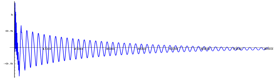
Figure 1: $\sqrt{2\pi n}\,T_{n}$, $1\leq n\leq 800$

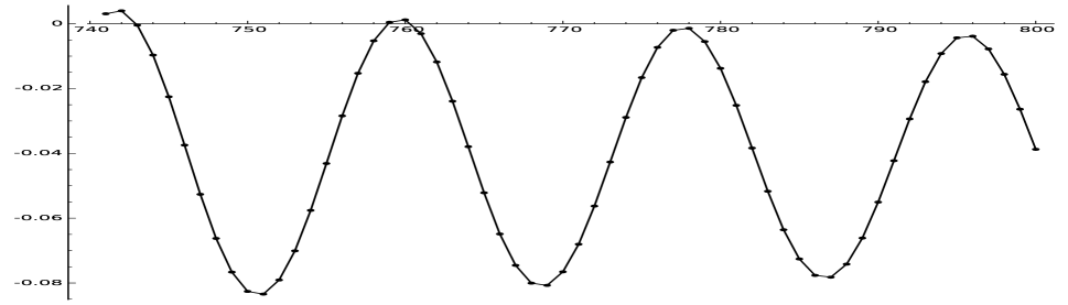
Figure 2: $\sqrt{2\pi n}\,T_{n}$, $740\leq n\leq 800$

Clearly $Y$ “nearly” has span 17, so that the graph is the result of applying a damping function to a function that is periodic of period 17. However, at $n_{0}=761$ the damping finally forces to the tilt to become, and forever stay, negative. The actual numerical values in the vicinity of $n_{0}$, and the next local maxima, are:

$$\begin{array}[]{rrrrr}n&759&760&761&762\\ \sqrt{2\pi n}\,T_{n}&0.000439&0.001195&-0.003066&-0.011796\\ &&\cdots&&\\ n&776&777&778&779\\ \sqrt{2\pi n}\,T_{n}&-0.007300&-0.002028&-0.001415&-0.005505\\ \end{array}$$

The size of the tail bound near $n_{0}$ was a surprise to us; it is 15 times the size of the principal error term. Moreover, we had thought that Corollary 12 shifted the extreme tail bound to an exponential term of the form $e^{-cn}$ rather than $e^{-c\sqrt{n}}$, and that this would be good enough. The key point is of course that the constant $r$ is uncomfortably small. We wondered whether the alternate $r$ in [Ben75] would be better, but in the case of $Y$ Benedick’s constant is very slightly worse than ours, and gives essentially the same $n_{2}$. We tried to replace $r$ with the optimal value

$$r_{\rm opt}=\min_{t\in[-\pi,\pi]}\frac{1-|f(t)|}{t^{2}}.$$

This gave a factor of improvement to $n_{2}$ of somewhat more than 2:

$$\begin{array}[]{lcr}&r&n_{2}\\ \mbox{Benedicks}&.0026144\ldots&194{,}081\\ \mbox{ours}&.0028144\ldots&182{,}024\\ \mbox{optimal}&.0055834\ldots&88{,}181\\ \end{array}$$

The graph of the absolute value $|f(t)|$ of the CF shows what the problem is. The goal is to find an upper bound for the integral of $|f(t)|^{n}/t$ outside $[-1/\sigma,1/\sigma]$, as $n$ gets large. The function $1-rt^{2}\leq e^{-rt^{2}}$ is a natural choice, but does not work well for a characteristic function whose secondary peaks are so high.

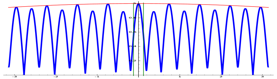
Figure 3: $|f_{Y}(t)|$

There are several things that can be done to improve the bound on the tail integral. The following extremely simple device made a dramatic improvement compared to the $n_{2}$ given above. The heights of the peaks in the graph of $|f(t)|$ (starting from $0$ and moving to the right) are

$$1,0.88989,0.99645,0.89768,0.98621,0.91204,0.97048,0.93077,0.95118.$$

The third peak is dominant. It occurs at $t=t_{0}=4\pi/17$ and has height $h_{0}=.99645$. The fifth peak has height $h_{1}=.98621$ and is the second most dominant peak. Let $f^{*}$ be the function that is the constant $h_{1}$ on $[-\pi,-1/\sigma]\cup[1/\sigma,\pi]$ except for the small section of the parabola $h_{0}\cdot(1-34(t-t_{0})^{2})$ that is above the line $y=h_{1}$, and the mirror image of this parabola section at $t=-t_{0}$. One can check that $f^{*}$ is an upper bound on $|f|$ outside of $[-1/\sigma,1/\sigma]$, and it is easy to estimate the integral of $f^{*}(t)^{n}/|t|$ on $1/\sigma\leq|t|\leq\pi$.

Using this tail bound we get an improved $n_{2}^{\prime}=1455$, which was much smaller than we had expected. The only significant contributions to the error are the $2q_{2}/n$ term and the tail bound, which are, respectively, $0.02766$, and $0.012709$ so that the total error is just less than $|L|$:

$$0.0276602867+0.01270946=.040370408<|L|=.0404226.$$

All other contributions to the error are less than $10^{-6}$, and the tail bound has been reduced to under half of the primary contribution.

One can push this further by considering all of the peaks and lowering the “threshold” to, say, the value of the CF at $1/\sigma$, i.e., the value of the normalized CF $g(t)$ at $t=1$. This seems to move $n_{2}^{\prime}$ further down to an $n_{2}^{\prime\prime}$ just above 1200 (and we think that this is about the limit of what can be done). However, the time required to program this correctly far exceeds the time that a computer takes to compute the tilts between 1200 and 1455, so our general philosophy says that it would be silly to implement this improvement.

Finally, we consider an example that originally motivated this investigation. Consider three nontransitive dice, that appeared in one of Martin Gardner’s columns many years ago, whose PGFs are

$$A=(z^{2}+z^{6}+z^{7})/3,\qquad B=(z^{1}+z^{5}+z^{9})/3,\qquad C=(z^{3}+z^{4}+z^{8})/3.$$

Write $A>B$ to mean that ${\bf Pr}(A>B)>{\bf Pr}(B>A)$, i.e., it is more likely that a roll of $A$ is larger than a roll of $B$ than the reverse. This is the same thing as saying that the tilt $T(A-B)$ of the difference $U=A-B$ is positive. Note that the PGF of $U$ is $A(z)B(z^{-1})$. Similarly, let $V=B-C$ and $W=C-A$. It turns out that

$$A>B,\;B>C,\;C>A,\quad\mbox{whereas}\quad A[2]<B[2],\;B[2]<C[2],\;C[2]<A[2].$$

In fact, the various dominance orders oscillate until $n=n_{0}=8$ when $A$ becomes dominant, and $B$ dominates $C$, in the sense that

$$A[n]>B[n],\;A[n]>C[n],\;B[n]>C[n],\quad\mbox{for all}\quad n\geq n_{0}.$$

This can be verified by computer for $n$ as large as your hardware can go, but to prove that asymptopia arrives at $n_{0}=8$ we use Theorem 18. It turns out that

$$U(z)=A(z)B(z^{-1})=B(z)C(z^{-1})=V(z)$$

so there are really only two dice to which that theorem has to be applied: $U$ and $W$. By now we can give a guess as to how large $n$ will have to be, namely, we find the needed error $|L|$ and then choose $n$ large enough so that

$$\sqrt{2\pi n}\;T_{n}\simeq\sqrt{2\pi n}\;\frac{2q_{2}}{n}<|L|,\;\mbox{i.e.},\quad n>\frac{8\pi q_{2}^{2}}{L^{2}}.$$

Since $q_{2}=1/5+\nu_{4}/24$, for many random variables it is reasonable to bound $q_{2}$ by $1/4$, so that $n$ has to be at least as large as $\pi/(2L^{2})$.

For $W$ we find that $L=0.033310\ldots$, which is unusually small. The approximation $n\simeq 8\pi q_{2}^{2}/L^{2}$ suggests $n_{0}\leq 1407$, and in fact in this case $L$ is so small that $n$ is large enough so that all other terms of the error are negligible. In other words, the $n$ required by the principal error term so large that this gives the best possible value.

For $U$, the limit $L$ is larger, namely $L\simeq-0.14028\ldots$. In this case the bound implied by the principal term is $n=83$. Although the main tail bound term is then large, we can apply the earlier techniques of piecewise bounding the characteristic function, to show that $n_{0}\leq 83$. In other words, this shows that the smallest possible bound is achievable with a bit more work.

All of the above experiments are summarized in the following table.

$$\begin{array}[]{rrrrrrr}&L&n_{0}&n_{1}&n_{2}&n_{2}^{\prime}&n_{2}^{\prime\prime}\\ \hline\cr X_{0}&-0.16446&4&59&74&&\\ X_{1}&0.43856&5&9&37&&\\ X_{2}&-0.16446&2&59&70&&\\ X_{3}&-0.76748&3&3&27&&\\ Y&-0.040422&761&682&182{,}024&1455&1206\\ U&-0.14028&9&83&1933&83&\\ W&0.03333&5&1407&4591&1407&\\ \end{array}$$

where $n_{2}^{\prime}$ is the result of replacing the tail bound using a little bit of work (e.g., roughly where one could imagine that the necessary estimates could be verified by hand, as in the simple improvement for $Y$ above), and $n_{2}^{\prime\prime}$ is the result of replacing the tail bounds by bounds that require a computer to perform all of the verifications, as in the more complicated improved estimate for $Y$ earlier.

We close with some further comments.

1. The primacy of the $1/n$ term is a surprise. If we take the “poor man’s approximation” $q_{2}\simeq 1/4$, which is a good approximation unless $X$ takes very large values with very small probability, then the error is about $1/2n$, independent of $X$! And this says that the lower bound $n_{1}$, and often the arrival bound $n_{2}$, is almost entirely determined by the target error $|L|$. As a first guess, $n_{2}\simeq\pi/(2L^{2})$, especially if this number is large enough so that the exponential terms are small; if this approximation to $n_{2}$ isn’t that large then further work might be required to decrease the tail bound.

2. A curious philosophical difficulty is hiding in the weeds. The value of $n_{0}$ becomes “obvious” from calculations when the sign of the tilt becomes constant and stays there for as large an $n$ as one cares to compute. However, this gives no hint of how one might prove that this will continue to be the case, and the point of the work here is to be able to actually prove an upper bound on $n_{0}$. What computer results are admissible in such a proof? The computation of tilts would seem innocuous to many since any floating point error can be easily bounded, and the programs are short and “easily” proved to be correct — the computer is “just” doing stable, well-understood arithmetic . The error bounds in calculating $n_{2}$ straight from Theorem 18 can be done by hand, and perhaps the estimates for $n_{2}^{\prime}$ could also be done by hand, though few, if any people would do them nowadays without using a computer; the calculations needed to support the determination of $n_{2}^{\prime\prime}$ seem to be intrinsically even more demanding.

3. It would be interesting to apply these ideas here to more general situations (more general RVs, approximation not at the mean, etc.). Extending to higher order Edgeworth approximations seems viable, but would require algebraic stamina. We have thoughts on how this might be automated. However, as noted earlier, we expect that the lower bounds on $n$ will have to increase, so that the utility of this approach isn’t entirely clear.

Acknowledgments. We would like to thank Richard Arratia, Steve Butler, Persi Diaconis, Larry Goldstein, Fred Kochman, and Sandy Zabell for interesting and useful feedback.

References

- [Ben75] Michael Benedicks, An estimate of the modulus of the characteristic function of a lattice distribution with application to remainder term estimates in local limit theorems, Ann. Probability 3 (1975), 162–165.
- [BGH16] J.P. Buhler, R.L. Graham, and A.W. Hales, Maximally nontransitive dice, Preprint, 2016.
- [BR10] Rabi N. Bhattacharya and R. Ranga Rao, Normal approximation and asymptotic expansions, Society for Industrial and Applied Mathematics (SIAM), Philadelphia, PA, 2010.
- [Fel71] William Feller, An introduction to probability theory and its applications. Vol. II., Second edition, John Wiley & Sons, Inc., New York-London-Sydney, 1971.
- [Pet95] Valentin V. Petrov, Limit theorems of probability theory, Oxford Studies in Probability, The Clarendon Press, Oxford University Press, New York, 1995.