Spectral properties from Matsubara Green’s function approach — application to molecules

Abstract

We present results for many-body perturbation theory for the one-body Green’s function at finite temperatures using the Matsubara formalism. Our method relies on the accurate representation of the single-particle states in standard Gaussian basis sets, allowing to efficiently compute, among other observables, quasiparticle energies and Dyson orbitals of atoms and molecules. In particular, we challenge the second-order treatment of the Coulomb interaction by benchmarking its accuracy for a well-established test set of small molecules, which includes also systems where the usual Hartree-Fock treatment encounters difficulties. We discuss different schemes how to extract quasiparticle properties and assess their range of applicability. With an accurate solution and compact representation, our method is an ideal starting point to study electron dynamics in time-resolved experiments by the propagation of the Kadanoff-Baym equations.

I Introduction

Many-body perturbation theory (MBPT) is one of the most important tools for the prediction of electronic structures from first principles Mahan (2000). The controllability of approximations derived from diagrammatic techniques, the wealth of information about the spectroscopic observables contained in the single-particle Green’s function, and the compatibility of the method with the time-propagation and the description of transport properties are believed to be the strong points of the Green’s function approach. However, technical realization of these advantages has proved difficult.

In this work we focus on the extraction of spectral information encoded in the Matsubara Green’s function and on the benchmarking of a popular second Born approximation (2BA) for the self-energy. This study is motivated by the fact that the solution of the Dyson equation on the imaginary time-track is the first step of a typical nonequilibrium Green’s function (NEGF) approach in the two-times plane Balzer and Bonitz (2012); Stefanucci and Leeuwen (2013). The power of the NEGF approach has been demonstrated by the description of ultra-fast carrier dynamics Haug (1992); Vu and Haug (2000); Vu et al. (2006); Eckstein and Werner (2013), time-resolved photoemission Kemper et al. (2013); Sentef et al. (2013); Kemper et al. (2014); Schüler et al. (2016) and photoionization of atoms and molecules Balzer et al. (2010a, b). Some of these results were obtained by starting from the non-interacting reference state and switching on the interaction adiabatically. The numerical scheme simplifies significantly in this case. However, it requires the propagation up to longer times, increasing the computer memory requirements and the computational time considerably Balzer et al. (2012). Therefore, an efficient NEGF solver necessarily incorporates the vertical track of the Keldysh contour (Fig. 1) in the propagation scheme .

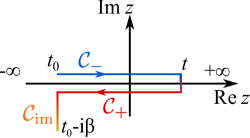
Figure 1: (Color online) Time-arguments of the electron Green’s function belong to the general contour $\mathcal{C}$ consisting of the forward branch $\mathcal{C}_{-}$ on the real axis, the backward branch $\mathcal{C}_{+}$ and the imaginary branch $\mathcal{C}_{\mathrm{im}}$. The arrows indicate the direction of the contour-ordering. $\beta$ denotes the inverse temperature.

Our choice of an approximation for the self-energy — the second Born approximation — has been shown to be relevant for molecular system Balzer et al. (2010a, b); Perfetto et al. (2015). In particular, exchange effects (the 2BA includes exchange up to second order) are known to have a significant contribution to the total energy  Marsman et al. (2009); Schäfer et al. (2017) — a fact that is elevated for molecular systems. In contrast to the broadly used (for equilibrium calculations) $GW$  Pavlyukh and Hübner (2004); Stan et al. (2009); van Setten et al. (2013, 2015); Kaplan et al. (2016) and the $T$-matrix approximations von Friesen et al. (2009); Puig von Friesen et al. (2010); Romaniello et al. (2012), it possesses an additional benefit of the time-locality. By this we mean that the self-energy $\Sigma(z_{1},z_{2})$ is a functional of the Green’s function with the same time-arguments. This simplifies the time-propagation considerably.

Many-body approximations have been tested extensively in the energy domain and used as the initial step for the time-propagation von Friesen et al. (2009); Balzer et al. (2010b, a); Hopjan et al. (2016). Direct construction of the initial propagator on the Keldysh contour is less common. Extensive study of the spectral properties of the 2BA theory have been performed on finite lattice systems based on the Pariser–Parr–Pople model Säkkinen et al. (2012). 2BA shows a clear improvement over the Hartree-Fock (HF) electronic structure: predicting in accordance with the exact diagonalization results the correlation-induced satellites, and yielding correct shifts of spectral features as a function of the interaction strength. However, oscillatory noise-like features, as well as broadening of the peaks in the frequency domain appear due to the finite propagation length in time-domain. How spectral features are reproduced in realistic systems, and how 2BA compares with standard quantum chemistry methods are still two open prominent questions. Some steps in answering these questions have been undertaken recently focusing on the integral properties. The importance of proper frequency grid for the representation of Matsubara Green’s function (MGF) has been demonstrated by Kananenka et al. in a study of simple molecular systems Kananenka et al. (2016a). They proposed a method based on spline interpolation and established a criterion determining the accuracy of the results. However, here we focus on the intrinsic limitations of the 2BA rather than on the errors induced by the numerical procedure.

In addition to already mentioned restrictions induced by the finite grid representation of the MGF, the extraction of the spectral properties from the imaginary time propagation is a nontrivial mathematical problem. The maximum entropy and the generalized Padé approximation have been compared with the direct Laplace transform by Dirks et al. Dirks et al. (2013). While on the conceptual level the former method is superior, it was suggested that the actual performance for realistic systems is rather subtle depending on the choice of the self-energy approximation. This is our second motivation for the benchmarking of various approaches for small molecules from the well established test sets and comparing the performances of the 2BA and the coupled-cluster approach. In this work, we analyze the closed-shell neutral molecules of the G2-1 set and the non-hydrogenic molecules from the G2/97 set Curtiss et al. (1997, 1998); Haunschild and Klopper (2012). The latter offers the advantage of directly comparing the 2BA to the $GW$ approximation from ref. Pham et al., 2013. The G2-1 test set also contains a number of molecules (such as the dimers Li₂, F₂, Na₂ and P₂) for which the electronic structure within the Hatree-Fock treatment differs considerably from the accurate coupled-cluster results. Thus, the limits of the 2BA as such and the extraction of quasiparticle properties can be assessed in an unbiased way.

As the last ingredient of this study we consider the extraction of the spectral information from the MGF using the extended Koopmans’ theorem (EKT) Chipman (1977). While extensive tests of this possibility have been performed in the quantum chemistry framework Vanfleteren et al. (2009), there has also been proposals to use EKT within the Green’s function approach Dahlen and van Leeuwen (2005); Stan et al. (2006). However, the EKT cannot be considered an equivalent substitute of the aforementioned spectral methods. While they use in principle all dynamical information encapsulated in the MGF, the latter approach solely relies on the one and two-particle density matrices and is sensitive to the asymptotic behavior of the bound state wave-functions Katriel and Davidson (1980). Because of this restriction, only the first ionization potential and electron affinity in each symmetry class can be obtained. However, the advantage is that EKT can be applied to any correlated ground state, e. g., from coupled cluster approaches.

The work is organized as follows. n Sec. II we summarize the well known self-energy expressions specializing on the Matsubara formalism, recall basic facts about the EKT, the analytic continuation (AC) and the Padé approximation, and describe the numerical implementation of these methods for molecular systems. In Sec. III the results of benchmark calculations are presented and compared with reference experimental and coupled cluster numerical data. In Sec. IV we discuss in details our main finding that the 2BA can compete with accurate quantum chemistry methods and thus endorse the method as accurate and extendible approach to equilibrium and excited-state properties of molecules.

II Methods

Our calculations are performed in the molecular orbital basis. Its size will be denoted as $N_{\text{bas}}$. Correspondingly, the MGF $\mathbf{G}(\tau)$ and self-energy $\mathbf{\Sigma}(\tau)$ are matrices related by the Dyson equation

$$\mathbf{G}(\tau)=\mathbf{g}(\tau)+\int^{0}_{-\beta}\!\mathrm{d}\tau_{1}\!\int^{0}_{-\beta}\!\mathrm{d}\tau_{2}\,\mathbf{g}(\tau-\tau_{1})\mathbf{\Sigma}(\tau_{1}-\tau_{2})\mathbf{G}(\tau_{2})\ .$$ (1)

Here $\mathbf{g}(\tau)$ is the reference Green’s function

$$g_{ij}(\tau)=\delta_{ij}\left[(n_{i}-1)\theta(\tau)+n_{i}\theta(-\tau)\right]e^{-(\varepsilon_{i}-\mu)\tau},$$ (2)

with $n_{i}=n_{\mathrm{F}}(\varepsilon_{i}-\mu)$ ($n_{\mathrm{F}}(\omega)\equiv(1+e^{\beta\omega})^{-1}$ denotes the Fermi distribution function), and $\varepsilon_{i}$ standing for the HF eigenvalues. Introducing the Coulomb matrix elements

$$\left(il|kj\right) =\int\!\mathrm{d}\mathbf{r}\!\!\int\!\mathrm{d}\mathbf{r}^{\prime}\,\phi^{*}_{i}(\mathbf{r})\phi^{*}_{j}(\mathbf{r}^{\prime})\mathscr{v}(\mathbf{r}-\mathbf{r}^{\prime})\phi_{k}(\mathbf{r}^{\prime})\phi_{l}(\mathbf{r}),\$$

the constituent second order self-energy can be efficiently computed using the matrix multiplication:

$$\Sigma^{(2)}_{ij}(\tau)=\sum_{klmnpq} \left(ik|mq\right)\left(lj|pn\right)\Big{[}2G_{kl}(\tau)G_{mn}(\tau)G_{pq}(-\tau)$$

$$\quad-G_{kq}(\tau)G_{mn}(\tau)G_{pl}(-\tau)\Big{]}\ ,$$ (3)

While this does not change the complexity proportional to the fifth power of the number of basis functions ($\mathcal{O}(N_{\text{bas}}^{5})$), the use of specialized libraries and parallelization allows to achieve a substantial speed up (the brute force approach leads to $\mathcal{O}(N_{\text{bas}}^{8})$ scaling Balzer et al. (2012)). Another possibility to increase the performance would be to use the finite-element discrete variable representation, which was shown to lead to $\mathcal{O}(N_{\text{bas}}^{4})$ scaling Balzer et al. (2010b).

The Dyson equation (1) is typically Fetter and Walecka (2003) solved by Fourier-transforming $\mathbf{G}(\tau)$ to imaginary frequencies $\omega_{m}$,

$$\widetilde{\mathbf{G}}(\mathrm{i}\omega_{m})=\int^{\beta}_{0}\!\mathrm{d}\tau\,\mathbf{G}(\tau)e^{\mathrm{i}\omega_{m}\tau},\quad\omega_{m}=\frac{(2m+1)\pi}{\beta}\ ,$$ (4)

yielding an algebraic Dyson equation. The self-energy is, however, most efficiently evaluated in $\tau$-space. Hence, switching back and forth between time and frequency representation is the standard implementation of the self-consistency cycle. Due to the non-continuous behavior of the MGF at $\tau=0$, the Fourier coefficients $\widetilde{\mathbf{G}}(\mathrm{i}\omega_{m})$ behave as $(\mathrm{i}\omega_{m})^{-1}$ for large $|m|$. This slow convergence introduces significant numerical errors which are countered by tail corrections. However, the standard first-order correction scheme Aoki et al. (2014) still requires a typical number of thousands of frequencies $\mathrm{i}\omega_{m}$ to achieve accurately converged results. Higher-order tail corrections Kananenka et al. (2016a) is a promising perspective to improve the efficiency of this scheme.

An alternative approach is to solve the Dyson equation directly as integral equation. By replacing the integration over the imaginary time arguments by a suitable quadrature with points $\tau_{p}$ and weights $w_{p}$, the integral equation (1) is recasted into a system of linear equations Balzer et al. (2009):

$$\sum^{N_{\mathrm{quad}}}_{q=1}\left[\mathbf{I}\delta_{pq}-w_{q}\mathbf{Z}(\tau_{p},\tau_{q})\right]\mathbf{G}(\tau_{p})=\mathbf{g}(\tau_{p})$$ (5)

with integral kernel

$$\mathbf{Z}(\tau,\tau^{\prime})=\int^{0}_{-\beta}\!\mathrm{d}\tau^{\dprime}\,\mathbf{g}(\tau-\tau^{\dprime})\mathbf{\Sigma}(\tau^{\dprime}-\tau^{\prime})\$$

Combining $N_{\mathrm{bas}}$ basis and $N_{\mathrm{quad}}$ grid indices into a multi-index, Eq. (5) is transformed into a $N_{\mathrm{bas}}N_{\mathrm{quad}}$-dimensional system of linear equations with $N_{\mathrm{bas}}$ right-hand sides. Solving the Dyson equation directly as integral equation yields a solution free of high-frequency artefacts. By evaluating eq. (5) and (II) by higher-order quadrature schemes  , we obtain a highly accurate solution even for moderate number of grid points $\tau_{p}$. The numerical bottleneck of the method is the additional computational cost of constructing the kernel (II). However, its calculation can be efficiently incorporated into a distributed memory scheme for solving the linear equation (5), giving rise to excellent scaling with the number of processing cores. We remark that the MGF obtained by the solving in the frequency space can provide a good initial guess for $\mathbf{G}(\tau)$ to be inserted in the right-hand side of eq. (1). Constructing an improved MGF from the left-hand side and substituting back into the convolution on the right-hand side constitutes an iterative solution of the Dyson equation Schüler et al. (2017).

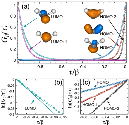
Figure 2: (Color online) (a) Typical behavior of MGF as a function of imaginary time $-\beta<\tau<0$, $G_{ik}(\tau)=-G_{ik}(\tau+\beta)$ for the CH₂ molecule as an example. The circles represent the grid points used in the calculations. The insets depict the molecular orbitals corresponding to the diagonal matrix elements $G_{ii}(\tau)$. On the panels below, we compare the MGF obtained by solving the Dyson equation using the HF self-consistent procedure (circles) and the MGF reconstructed from energies and states of the EKT eigenproblem (9) (full lines) for the LUMO (b) and the occupied valence orbitals (c).

In order to deal with cusps at the boundaries $\tau=-\beta$ and $\tau=0$ while retaining a compact representation of the MGF, we employ a grid $\tau_{p}$ with exponentially increased density at the boundaries (Fig. 2(a)). The exponential scaling is optimized to best represent the (noninteracting) MGF corresponding to highest occupied molecular orbital (HOMO). For achieving converged results, we typically need $N_{\mathrm{quad}}=200$ to $N_{\mathrm{quad}}=300$ grid points.

We have implemented three different levels of self-consistency at which the Matsubara GF is determined:

• the non-self-consistent (non-sc) treatment, where the Dyson equation is solved only once using the self-energy constructed from the reference Hartree-Fock (HF) Green’s function;

• the partially self-consistent scheme where only the mean-field part of the Hamiltonian is updated (HF-sc) until the convergence of the MGF;

• the fully self-consistent scheme (full-sc), where the Dyson equation is solved and the self-energy is constructed repeatedly until the convergence of the MGF is achieved.

The convergence is achieved when the norm of deviation of $\mathbf{G}(\tau)$ between subsequent iteration steps for all imaginary time arguments $\tau_{p}$ is below a specified threshold. This criterion is more stringent than the convergence of the density matrix, which corresponds to the value of MGF at $\tau=0$.

Direct extraction of the spectral function $A_{ik}(\omega)$ from the MGF amounts to solving the integral equation

$$\mathbf{G}(\tau) =\int\!\frac{\mathrm{d}\,\omega}{2\pi}\mathbf{A}(\omega)\frac{e^{-\tau\omega}}{1+e^{-\beta\omega}},$$ (6)

which is a nontrivial task Dirks et al. (2013). That is why we explore the AC and the EKT routes.

Analytic continuation

transforms the Green’s function of the imaginary time argument $\tau$ into the function of complex frequency $\zeta$ in a sequence of two steps $\mathbf{G}(\tau)\rightarrow\widetilde{\mathbf{G}}(\mathrm{i}\omega_{m})\rightarrow\widetilde{\mathbf{G}}(\zeta)$. For $\zeta$ in the vicinity of real axis, the latter quantity relates to retarded/advanced GFs ($\widetilde{\mathbf{G}}(\omega\pm\mathrm{i}\eta)=\mathbf{G}^{\mathrm{R/A}}(\omega+\mu)$) and yields the spectral function according to

$$\mathbf{A}(\omega) =\mathrm{i}\left[\widetilde{\mathbf{G}}(\omega-\mu+\mathrm{i}\eta)-\widetilde{\mathbf{G}}(\omega-\mu-\mathrm{i}\eta)\right]_{\eta\rightarrow 0^{+}}\ .$$

For equidistant grids in imaginary time, fast Fourier transformation to the imaginary frequency domain is the standard procedure. However, for our efficient solution scheme of the Dyson equation — which relies on an optimized non-equidistant grid of $\tau$-points — it is more efficient to employ an orthogonal polynomial representation Kananenka et al. (2016b). The Fourier coefficients of the Matsubara GF (4) are computed by representing the function in terms of Legendre polynomials $P_{n}(x)$:

$$\mathbf{G}(\tau)=\frac{1}{\beta}\sum^{\infty}_{n=0}\sqrt{2n+1}\,\,P_{n}\left(\frac{2\tau}{\beta}-1\right)\mathbf{C}_{n}\ ,$$ (7)

yielding Boehnke et al. (2011)

$$\widetilde{\mathbf{G}}(\mathrm{i}\omega_{m})=(-1)^{m}\sum^{\infty}_{n=0}\mathrm{i}^{n+1}\sqrt{2n+1}\,\,j_{n}\left(\frac{1}{2}\beta\omega_{m}\right)\mathbf{C}_{n}\ .$$ (8)

Here $j_{n}(x)$ denotes the spherical Bessel function of the first kind. On the second step, the complex function $\widetilde{\mathbf{G}}(\zeta)$ is represented by its Padé approximant constructed from the points $\mathrm{i}\omega_{m}$. In practice, the order of the Legendre polynomials is truncated at $\simeq 64$, yielding excellent accuracy. The order of the Padé approximation (we choose 28) plays only a minor role.

Extended Koopmans’ theorem

One quantity immediately available from MGF is the density matrix $\boldsymbol{\gamma}^{\pm}=\mathbf{\lim}_{\tau\rightarrow 0^{\pm}}\mathbf{G}(\tau)$ (upper/lower sign for particle/hole density, respectively). Computation of the quasiparticle excitations additionally requires the two-body correlation function as encoded in the first derivative $\mathbf{\Delta}^{\pm}=-\lim_{\tau\rightarrow 0^{\pm}}\partial_{\tau}\mathbf{G}(\tau)$ Dahlen and van Leeuwen (2005); Stan et al. (2006). With these two ingredients a generalized eigenvalue problem

$$\mathbf{\Delta}^{\pm}\mathbf{u}^{\pm}_{\alpha}=\epsilon^{\pm}_{\alpha}\boldsymbol{\gamma}^{\pm}\mathbf{u}^{\pm}_{\alpha}$$ (9)

yields the quasiparticle energies $\epsilon^{\pm}_{\alpha}$. Corresponding Dyson orbitals can be obtained from the normalized ($\left[\mathbf{u}^{\pm}_{\alpha}\right]^{\dagger}\boldsymbol{\gamma}^{\pm}\mathbf{u}^{\pm}_{\beta}=\delta_{\alpha,\beta}$) eigenvectors as follows $\boldsymbol{\phi}^{\pm}_{\alpha}=\boldsymbol{\gamma}^{\pm}\left(\mathbf{u}^{\pm}_{\alpha}\right)^{*}$. In terms of $\epsilon^{\pm}_{\alpha}$ and $\boldsymbol{\phi}^{\pm}_{\alpha}$, the spectral function is given by:

$$\mathbf{A}(\omega)=2\pi\sum_{i=\pm}\sum_{\alpha}\left[\boldsymbol{\phi}^{i}_{\alpha}\right]^{\dagger}\boldsymbol{\phi}^{i}_{\alpha}\delta(\omega-\epsilon^{i}_{\alpha}).$$ (10)

Let us remark on the relation of the AC and the EKT. Provided one has found an exact MGF (by exact diagonalization, for instance), the EKT reproduces (in the limit $\beta\rightarrow\infty$) the exact many-body energies. The same is true for the AC. At the level of finite-order MBPT, the relation is less clear. Low-order diagrammatic methods such as the 2BA or the $GW$ approximation result in additional features like satellites and broadening, which can not be captured by the EKT. A typical example where the simple exponential behavior of the MGF implied by the EKT (the Green’s function is reconstructed by substituting the spectral function (10) into the integral representation Eq. (6)) deviates from the self-consistent solution is shown in Fig. 2(b)–(c) for the lowest unoccupied molecular orbital (LUMO) and the occupied orbitals. One can expect that in case the effects of the 2BA is primarily given by shifting the HF energies, the EKT and resulting peaked spectral function (10) is an excellent approximation (as can be seen for the occupied orbitals), while it might give inconsistent results if the above mentioned features of MBPT come into play. For this reason, we employ both methods for obtaining quasiparticle properties and compare them.

Figure 3: (Color online) Ionization potentials of the G2-1 molecules (a)–(c) within the 2BA (using the EKT) and, for comparison, (d) within MP2 and (e) CCSD, vs. the experimental values (taken from ref. Johnson ). Values are in eV. Panel (f) shows the mean absolute error (MAE) for each method with respect to the experimental values; color coding is consistent with other panels.

III Electronic properties of G2 molecules

For a comprehensive benchmark, we study all 36 neutral closed-shell molecules from the G2-1 test set Curtiss et al. (1997) with geometries optimized at the B3LYP/6-31* level. The restricted HF calculation is performed using the aug-cc-pVDZ basis noa ; Feller (1996) as the starting point, all the matrix elements are transformed from the atomic to molecular orbital basis using our in-house code Pavlyukh and Berakdar (2013). In this basis the Dyson equation (1) is subsequently solved for the low-temperature case $\beta=80$ and spectral properties are determined. We tested the convergence of the results with respect to the basis size by introducing a cutoff energy $E_{\mathrm{cut}}$ such that $\varepsilon_{i}<E_{\mathrm{cut}}$ for all states $i$. In general, higher molecular orbitals are not described well by the Gaussian basis set, such that including them leads to additional errors. On the other hand, the molecular basis set needs to be large enough to describe adding an extra electron. We performed calculations for two values for the cutoff: $E_{\mathrm{cut}}=0.5$ a. u. and $E_{\mathrm{cut}}=1.5$ a. u., respectively. In what follows, we present the results for $E_{\mathrm{cut}}=1.5$ a. u., while the corresponding results for the smaller cutoff are summarized in Appendix A.

For comparison, the second-order Møller-Plesset perturbation theory (MP2) and the coupled-cluster method including single and double excitations (CCSD) is used. With these two reference methods, the total energies of the neutral and the positively/negatively charged ions were computed using the same basis set (aug-cc-pVDZ) and the active space, yielding accurate estimates to the vertical ionization potential (IP) and the electron affinity (EA) according to the energy difference method. It should be noted, however, that for some molecules the underlying HF calculation suffers from multi-configuration instabilities. In such cases, the HF ground state of the neutral or ionized system differs significantly from the true electronic state. We will come back to this point later.

III.1 Ionization potentials and electron affinities of G2-1 molecules

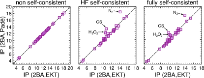
Figure 4: (Color online) Comparison of the ionization potentials obtained from the EKT and the Padé analytic continuation for three different levels of self-consistency. Values are in eV.

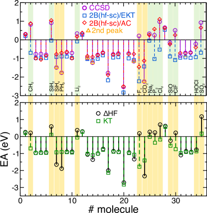
Figure 5: (Color online) Comparison of the electron affinities obtained from the HF self-consistent scheme using the extended Koopmans’ theorem (EKT, blue squares) and the Padé analytic continuation (AC, red diamonds) to the CCSD reference values. The orange triangles denote the second electron affinities. The yellow bars in the background indicate a significant discrepancy of $-\varepsilon_{\mathrm{LUMO}}$ (KT) to the EA computed by taking the difference of the total energy ($\Delta$HF). The cases with a good agreement between the EAs obtained from the Padé AC and the CCSD reference are marked green background bars.

In order to assess the performance of the 2BA, as compared to the reference methods, we computed the IPs and compared them to the experimental values in Fig. 3. The EKT (9) was used to extract the IPs from the MGF. Generally, the 2BA provides a quite accurate picture. Typical deviations from experimental values, which occur within MP2 and CCSD, as well, are not cured by the 2BA. This can be related to the above mentioned multi-configuration problems. In principle, these deficiencies can be rectified by starting from a multi-configurational HF to construct the reference GF $\mathbf{g}(\tau)$. As can already observed from the distribution of the IPs in Fig. 3(a)–(c), the non-sc scheme severely overestimates the IPs. Comparing with the initial restricted Hartree-Fock (RHF) values (which are mostly located under the diagonal), the non-sc treatment moves most of the points up and thus "overshoots" the QP shifts. The HF-sc level, on the other hand, yields much better results, which can be seen from the small distance of the points from the diagonal. Visually, the predictions of the IPs by the HF-sc scheme is very similar to the MP2 or CCSD reference. Switching to full self-consistency, Fig. 3(c), the values are slightly deteriorating with respect to the HF-sc level. Such oscillatory behavior of the MBPT and the levels of self-consistency is very typical. Similar behavior is also known for the $GW$ approximation, where partly self-consistent schemes such as $GW_{0}$ or quasiparticle self-consistency are typically superior to full-sc treatment.

For a quantitative analysis, we computed the mean absolute error (MAE) for each of the methods:

MAE $$=\frac{1}{N}\sum_{i=1}^{N}\left|E_{i}^{\text{c}}-E_{i}^{\text{r}}\right|.$$ (11)

Here the sum is performed over all systems, $E_{i}^{\text{c}}$ and $E_{i}^{\text{r}}$ refer to the computed and the reference data, respectively. As inferred from Fig. 3(f), the 2BA on non-sc level is not even better than the RHF (IPs from Koopmans’ theorem), because of the overestimated QP shifts, while the accuracy of the HF-sc scheme is comparable to the MP2 method. The quality of the full-sc treatment is on the intermediate level between the RHF and the MP2. In principle, the 2BA is expected to perform similarly to MP2, as both methods are of the second order in the Coulomb interaction. Due to the oscillatory nature of MBPT theory Pavlyukh (2017), however, the partially self-consistent (HF-sc) level performs the best.

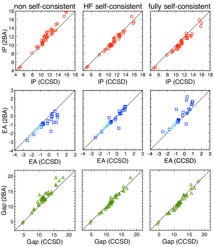
Figure 6: (Color online) Ionization potentials (top panels), electron affinities (middle panels) and band gaps (bottom panels) of the G2-1 molecules, obtained from the 2BA vs. the CCSD reference. Values are in eV. The Green’s function calculation are performed using $E_{\text{cut}}=1.5$ a. u. and the Padé approximation.

So far the IPs were computed using the EKT. As the next step we compared them to the IPs extracted from the AC accomplished by the Padé approximation (Fig. 4). Both methods yield almost identical values for non-sc case (left panel of Fig. 4). On the HF-sc and the full-sc levels, except for pathological cases such as the N₂, CS and H₂O₂ molecules, there are only some small deviations. N₂ and CS possess a triple bond leading to stronger electron localization and thus electronic correlation, making such systems difficult to treat. For instance, a diagrammatic expansion of the self-energy up to fourth order is needed Day (2007) to correctly capture the orbital structure of N${}^{+}_{2}$. For a low-order diagrammatic approach, such strong many-body effects result in a deviation from simple quasiparticle behavior which can not be captured by the EKT. Hence, there are pronounced differences of the IP obtained by the AC and the EKT. Similarly, the failure of Koopmans’ theorem (KT) for CS due to pronounced correlation effects is also known Ponzi et al. (2014). Apart from such cases, the IPs obtained by either method agree well.

The situation changes substantially for the electron affinities (Fig. 5). For a large class of molecules, the EKT provides a good estimate of the EA (we take CCSD as the reference). However, for some molecules (CH₂, SiH₂, Li₂, F₂, CO₂, Na₂, P₂, Cl₂, SiO, ClF, SO₂) the EA obtained by the EKT applied to the 2BA (HF-sc level) is very different from the reference. These discrepancies are reminiscent of the errors of the KT for the EAs within RHF. In fact, the EKT gives only small QP shifts from the initial RHF energy levels entering the reference MGF $\mathbf{g}(\tau)$. Hence, the EAs differ only little from $-\varepsilon_{\mathrm{LUMO}}$. The above molecules are typical cases where $-\varepsilon_{\mathrm{LUMO}}$ is a poor estimate for the EA (even within the RHF). Fig. 5 demonstrates that this behavior transfers to the EKT: the molecules where the KT prediction differs substantially from the more accurate estimation based on the total energy differences (the so-called $\Delta$HF method) are identical to those where the EA obtained by the EKT is quite off the CCSD reference value. However, employing the Padé approximation yields a substantial improvement, as the EAs obtained within the 2BA are much closer to the CCSD values. In particular, except for the F₂ and P₂ dimers, the Padé approximation always reproduces the correct sign of the respective EAs. In cases where the modulus of the EAs is underestimated as compared to CCSD, taking the second EAs (i. e. the second QP peak) leads to almost perfect agreement. This is a clear indication of the multi-configurational instability of the ground state of either the neutral or the negatively charged molecule. Such deficiencies related to the HF starting point can, in principle, be overcome by the full-sc treatment (as the dependence on the starting points disappears). However, converging the Dyson equation towards the self-consistency can be hindered by the multi-valuedness of the solution Stan et al. (2015); Tarantino et al. (2017).

Since several factors (besides the multi-configurational stability) contribute to the IPs and EAs measured in experiments, accurate methods like the CCSD can, of course, not yield perfect results. Most importantly, the restricted Gaussian basis set does describe excited orbitals well. In order to compare the methods on equal grounds, we show the IPs, EAs, and the resulting QP gap of the 2BA directly vs. the CCSD in Fig. 6. As for the IPs extracted by the EKT (Fig. 3), one can infer that the HF-sc scheme performs the best throughout; the agreement of the gaps between CCSD and the 2BA is especially good. It does not rely on the errors cancellation for the electron affinities (as illustrated in Fig. 5, see important exceptions) and ionization potentials, but is separately achieved for each quantity. Fig. 6 confirms that the 2BA on HF-sc level is almost comparable to the CCSD method.

We note that decreasing the basis cutoff to $E_{\mathrm{cut}}=0.5$ a. u. further improves — as expected — the agreement of the IPs with the CCSD method. However, the accuracy of the EAs is slightly deteriorated. The corresponding values are given in Appendix A. The overall performance of the different levels of self-consistency remains the same as for the larger cutoff.

III.2 Ionization potentials and electron affinities of G2/97 molecules

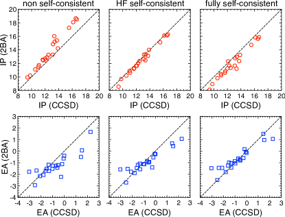
Figure 7: (Color online) Ionization potentials (top panels) and electron affinities (bottom panels) of the G2/97 molecules, obtained from the 2BA vs. the CCSD reference. Values are in eV. The Green’s function calculation are performed using $E_{\text{cut}}=0.5$ a. u. and the Padé approximation.

Analogous to the G2-1 molecules, we have also performed calculations for the non-hydrogenic closed-shell molecules from the G2/97 test set. Since the molecules are composed by of heavier elements, the number of valence orbitals and the HF basis increases considerably. In Fig. 7 the IPs and EAs computed using the Padé approximation and a basis determined by the cutoff $E_{\mathrm{cut}}=0.5$ a. u. are presented agaist the results of the CCSD method. Generally, a very good agreement is found. Especially the IP is well captured by the 2BA. Similarly to the results for the G2-1 molecules, the partially self-consistent scheme performs best for predicting the IP. Interestingly, the full-sc level improves the accuracy of the EAs for this smaller basis size. We have also tested $E_{\mathrm{cut}}=1.5$ a. u. (see Appendix B), which results in slightly better agreement of the EAs to the CCSD values at HF-sc level at the cost of slightly decreasing the accuracy of the IPs. For the full-sc scheme, on the other hand, both the IPs and the EAs deviate more from the CCSD as for the smaller cutoff. In any case, the HF-scheme performs best throughout and yields very good agreement with the CCSD reference for both values of the cutoff.

In Fig. 8 we compare the IPs within the 2BA treatment (HF-sc) and within the $G^{0}W^{0}$ approximation (values taken from ref. Pham et al., 2013) to experimental values. Both methods perform well; however, the MAE of 0.37 eV for the 2BA is considerably smaller than the MAE of 0.55 eV obtained from the $G^{0}W^{0}$ approach. This underlines that the 2BA is an excellent method for describing electronic properties of molecules.

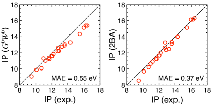
Figure 8: (Color online) Ionization potentials of the G2/97 molecules, comparing the $G^{0}W^{0}$ approximation from ref. Pham et al., 2013 (left panel) and the HF-sc 2BA (right panel) to experimental values. Values are in eV. The Green’s function calculation are performed using $E_{\text{cut}}=0.5$ a. u. and the Padé approximation.

IV Conclusions

We performed benchmark calculations using the second Born approximation for the electron self-energy of a number of molecular systems and found overall very good performance of the Matsubara Green’s function approach in comparison with correlated quantum chemistry methods. For all methods, the error is substantially smaller if systems with multi-configurational ground state are excluded. Same is true for $GW$ method Pavlyukh and Hübner (2007).

The partially self-consistent scheme has been demonstrated to perform the best throughout with a predictive power on par with quantum chemistry methods. Nevertheless, the fully self-consistent scheme performs very well for the majority of molecules, too. This is an important requirement for performing time-dependent calculations, allowing to compute, for instance, accurate optical absorption spectra. An alternative possibility would be to completely eliminate the Matsubara step and exploit the adiabatic switching scenario that can be further facilitated by the use of generalized Kadanoff-Baym Ansatz Galperin and Tretiak (2008); Pal et al. (2009); Ness and Dash (2011); Latini et al. (2014).

For extracting the quasiparticle properties we adopted two methods: the EKT and analytic continuation. They yield almost identical results for electron removal energies, the EKT was found to suffer from similar deficiencies as the KT within HF theory for around one third of the investigated molecules. This drawback can be cured by analytic continuation which yields excellent results for both ionization potentials and electron affinities.

As is mentioned in the introduction, there are several implementations of 2BA for systems ranging from atoms Dahlen and van Leeuwen (2005), to Hubbard Puig von Friesen et al. (2010); Hopjan et al. (2016) and Anderson Uimonen et al. (2011) models, to ultracold gases Schlünzen et al. (2016) and periodic systems Rusakov and Zgid (2016); Welden et al. (2016), also addressing the question of the accuracy of such calculations. Our study focuses on one missing aspect of such studies, namely the performance of the method for molecular system, as a quick way to initialize the time-dependent propagation of the Kadanoff-Baym equations. To this end, we specifically focused on the inherent accuracy of 2BA. For improving the general predictive power, two key issues have to be adressed: an accurate solution of the Dyson equation and systematic improvements of the basis. This first requirement is fulfilled by our efficient solution scheme, based on a compact grid representation of the MGF. Further improvements in this regard can be expected by working directly in the basis of orthogonal polynomials or an optimized sparse representation Shinaoka et al. (2017); Otsuki et al. (2017), which would allow studying considerably larger systems or higher-order MBPT. Promising routes speeding up the calculation for larger systems while keeping a accurate single-particle basis is the already mentioned use of specialized basis to represent the self-energy Balzer et al. (2010b) or stochastic sampling methods Neuhauser et al. (2016).

Finally we notice that similar to the quantum chemistry Kong et al. (2012) and solid-state case Marsman et al. (2009), the explicitly correlated R12/F12 approaches are expected to recover even a larger portion of the correlation energy in the Matsubara Green’s function method. This idea opens new prospects for further investigations.

Appendix A G2-1 molecules

In this section we present for completeness 2BA results for the molecules from the G2-1 set computed at the lower energy cutoff of $E_{\text{cut}}=0.5$ a.u. using the Padé approximation, Tabs. 1 and 2. For the CS molecule, the CCSD value for EA in aug-cc-pVDZ basis is not available; instead the CCSD(T)/cc-pVDZ value from the NIST Standard Reference Database is used Johnson .

Table 1: Ionization potentials of the molecules from the G2-1 set. The energy cutoff of $E_{\text{cut}}=0.5$ a.u. is used for the 2BA calculations.

No.	System	n-sc	HF-sc	full-sc	CCSD	Exp.
1	LiH	$8.17$	$7.72$	$7.65$	$7.90$	$7.90$
2	CH2	$10.84$	$10.06$	$9.88$	$10.41$	$10.35$
3	NH3	$11.73$	$10.43$	$10.28$	$10.74$	$10.07$
4	H2HO	$13.84$	$12.16$	$11.96$	$12.42$	$12.62$
5	HF	$17.64$	$15.79$	$15.56$	$15.92$	$16.03$
6	SiH2	$9.25$	$8.92$	$8.76$	$9.36$	$8.92$
7	SiH4	$13.16$	$12.46$	$12.35$	$12.69$	$11.00$
8	PH3	$10.58$	$10.00$	$9.87$	$10.36$	$9.87$
9	H2S	$10.47$	$9.92$	$9.72$	$10.13$	$10.46$
10	HCl	$12.98$	$12.41$	$12.20$	$12.48$	$12.74$
11	Li2	$4.92$	$5.13$	$2.62$	$5.18$	$5.11$
12	LiF	$12.94$	$10.90$	$10.51$	$11.31$	$11.30$
13	C2H2	$11.17$	$10.95$	$10.53$	$11.20$	$11.40$
14	C2H4	$10.27$	$9.70$	$9.53$	$10.44$	$10.51$
15	C2H6	$13.19$	$12.25$	$12.12$	$12.65$	$11.52$
16	HCN	$13.48$	$13.34$	$12.87$	$13.45$	$13.70$
17	CO	$15.12$	$13.94$	$13.48$	$13.80$	$14.01$
18	HCOH	$12.01$	$10.39$	$10.05$	$10.68$	$10.88$
19	CH3OH	$12.25$	$10.75$	$10.53$	$10.88$	$10.84$
20	N2	$16.73$	$14.91$	$14.30$	$15.45$	$15.58$
21	N2H4	$11.15$	$9.71$	$9.51$	$10.11$	$8.10$
22	H2O2	$13.16$	$10.86$	$10.39$	$11.43$	$10.58$
23	F2	$18.15$	$15.24$	$14.60$	$15.82$	$15.70$
24	CO2	$14.80$	$13.09$	$12.62$	$13.49$	$13.78$
25	Na2	$4.56$	$4.97$	$2.69$	$4.87$	$4.89$
26	P2	$10.12$	$10.25$	$9.47$	$10.31$	$10.53$
27	Cl2	$12.28$	$11.11$	$10.78$	$11.54$	$11.48$
28	NaCl	$9.57$	$8.62$	$8.46$	$8.93$	$9.20$
29	SiO	$11.90$	$10.71$	$10.71$	$11.37$	$11.49$
30	CS	$12.57$	$10.98$	$10.22$	$12.58$	$11.33$
31	ClF	$13.58$	$12.51$	$12.19$	$12.67$	$12.74$
32	Si2O6	$11.01$	$10.25$	$10.04$	$10.53$	$9.74$
33	CH3Cl	$11.87$	$11.00$	$10.75$	$11.20$	$11.26$
34	H3CSH	$9.73$	$9.00$	$8.75$	$9.24$	$9.44$
35	HOCl	$12.22$	$10.86$	$10.54$	$11.20$	$11.12$
36	SO2	$13.45$	$11.31$	$11.03$	$12.19$	$12.35$
MAE (eV)		$0.99$	$0.45$	$0.80$	$0.36$

Table 2: Electron affinities of the molecules from the G2-1 set. The 2BA calculations are performed at the energy cutoff of $E_{\text{cut}}=0.5$ a.u.

No.	System	n-sc	HF-sc	full-sc	CCSD
1	LiH	$0.23$	$0.27$	$0.30$	$0.30$
2	CH2	$-0.70$	$0.10$	$-0.82$	$0.83$
3	NH3	$-0.97$	$-0.87$	$-0.84$	$-0.77$
4	H2HO	$-0.96$	$-0.88$	$-0.85$	$-0.76$
5	HF	$-0.95$	$-0.92$	$-0.88$	$-0.80$
6	SiH2	$0.11$	$0.76$	$0.97$	$0.91$
7	SiH4	$-0.92$	$-0.81$	$-0.76$	$-1.49$
8	PH3	$-0.89$	$-0.69$	$-0.63$	$-1.77$
9	H2S	$-0.93$	$-0.73$	$-0.66$	$-0.67$
10	HCl	$-0.95$	$-0.79$	$-0.74$	$-0.71$
11	Li2	$-0.05$	$0.22$	$-0.43$	$0.34$
12	LiF	$0.27$	$0.30$	$0.32$	$0.32$
13	C2H2	$-1.02$	$-0.88$	$-0.80$	$-0.98$
14	C2H4	$-1.10$	$-0.97$	$-0.91$	$-1.23$
15	C2H6	$-1.00$	$-0.88$	$-0.83$	$-0.81$
16	HCN	$-0.79$	$-0.69$	$-0.61$	$-0.69$
17	CO	$-2.13$	$-2.03$	$-1.86$	$-1.78$
18	HCOH	$-0.90$	$-0.84$	$-0.77$	$-0.78$
19	CH3OH	$-0.92$	$-0.83$	$-0.78$	$-0.74$
20	N2	$-2.88$	$-2.73$	$-2.65$	$-2.53$
21	N2H4	$-0.97$	$-0.86$	$-0.80$	$-0.74$
22	H2O2	$-1.07$	$-0.96$	$-0.88$	$-1.15$
23	F2	$-1.78$	$-1.49$	$-1.07$	$0.21$
24	CO2	$-1.41$	$-1.23$	$-1.04$	$-2.24$
25	Na2	$0.00$	$0.29$	$2.23$	$0.33$
26	P2	$-0.35$	$0.17$	$1.02$	$0.25$
27	Cl2	$-0.17$	$-0.01$	$0.21$	$0.97$
28	NaCl	$0.57$	$0.59$	$0.62$	$0.66$
29	SiO	$-0.56$	$-0.39$	$-0.01$	$-0.14$
30	CS∗	$-1.27$	$-0.77$	$-0.18$	$-0.93$
31	ClF	$-0.75$	$-0.53$	$-0.32$	$0.51$
32	Si2O6	$-0.96$	$-0.74$	$-0.63$	$-0.86$
33	CH3Cl	$-0.90$	$-0.77$	$-0.70$	$-0.70$
34	H3CSH	$-0.94$	$-0.75$	$-0.67$	$-0.69$
35	HOCl	$-0.87$	$-0.70$	$-0.63$	$-0.22$
36	SO2	$0.18$	$0.32$	$1.14$	$0.93$
MAE (eV)		$0.44$	$0.23$	$0.49$

Appendix B G2/97 molecules

In this section we present for completeness 2BA results for the molecules from the G2/97 set computed at two different energy cutoffs $E_{\text{cut}}=0.5$ a.u. (Tabs. 5 and 6) and $E_{\text{cut}}=1.5$ a.u. (Tabs. 3 and 4) using the Padé approximation. There are no reliable experimental data for electron affinities of the molecules reported Tabs. 6 and 4. Therefore, we use CCSD results as reference for the computation of MAE.

Table 3: Ionization potentials of the molecules from the G2/97 set. The energy cutoff of $E_{\text{cut}}=1.5$ a.u. is used for the 2BA calculations.

No.	System	n-sc	HF-sc	full-sc	$G^{0}W^{0}$	CCSD	Exp.
1	BF3	$18.08$	$15.35$	$14.72$	$15.12$	$16.15$	$15.96$
2	BCl3	$12.48$	$11.19$	$10.43$	$11.37$	$11.69$	$11.62$
3	AlF3	$17.27$	$14.54$	$13.99$	$14.34$	$15.54$	$15.45$
4	AlCl3	$12.73$	$11.55$	$10.96$	$11.59$	$12.00$	$12.01$
5	CF4	$18.65$	$15.57$	$14.79$	$15.38$	$16.53$	$16.20$
6	CCl4	$12.55$	$11.03$	$10.02$	$11.22$	$11.64$	$11.69$
7	COS	$11.54$	$10.75$	$9.90$	$11.01$	$11.01$	$11.19$
8	CS2	$10.21$	$9.68$	$8.55$	$9.89$	$9.78$	$10.09$
9	CF2O	$15.21$	$12.52$	$11.81$	$12.91$	$13.40$	$13.60$
10	SiF4	$18.52$	$15.73$	$15.09$	$15.38$	$16.68$	$16.40$
11	SiCl4	$12.92$	$11.57$	$11.53$	$11.58$	$12.10$	$12.06$
12	N2O	$13.26$	$11.93$	$10.76$	$12.23$	$12.49$	$12.89$
13	ClNO	$11.76$	$10.43$	$8.77$	$11.29$	$11.08$	$10.94$
14	NF3	$15.39$	$12.68$	$11.71$	$13.07$	$13.73$	$13.60$
15	PF3	$12.89$	$11.75$	$11.20$	$11.85$	$12.27$	$12.20$
16	O3	$13.30$	$10.85$	$n.a.$	$12.20$	$13.10$	$12.73$
17	F2O	$16.02$	$12.07$	$10.83$	$12.75$	$13.35$	$13.26$
18	ClF3	$14.85$	$11.98$	$12.24$	$12.62$	$13.16$	$12.77$
19	C2F4	$11.12$	$9.69$	$8.85$	$10.08$	$10.53$	$10.69$
20	C2Cl4	$9.92$	$8.62$	$7.42$	$9.07$	$9.38$	$9.50$
21	CF3CN	$14.21$	$13.55$	$12.46$	$13.30$	$13.88$	$14.30$
MAE (eV)		$1.14$	$0.77$	$1.50$	$0.55$	$0.18$

Table 4: Electron affinities of the molecules from the G2/97 set. The energy cutoff of $E_{\text{cut}}=1.5$ a.u. is used for the 2BA calculations.

No.	System	n-sc	HF-sc	full-sc	CCSD
1	BF3	$-1.18$	$-1.00$	$-0.85$	$-1.35$
2	BCl3	$-1.20$	$-0.10$	$0.88$	$-0.53$
3	AlF3	$-0.38$	$-0.11$	$0.12$	$0.00$
4	AlCl3	$-0.65$	$-0.02$	$0.49$	$-0.06$
5	CF4	$-2.05$	$-1.78$	$-1.56$	$-1.79$
6	CCl4	$-1.42$	$-0.47$	$n.a.$	$-0.60$
7	COS	$-1.53$	$-1.09$	$-0.40$	$-1.52$
8	CS2	$-1.13$	$0.19$	$1.66$	$-0.18$
9	CF2O	$-1.67$	$-1.32$	$-1.00$	$-2.39$
10	SiF4	$-1.26$	$-1.00$	$-0.80$	$-0.97$
11	SiCl4	$-1.25$	$-0.69$	$n.a.$	$-0.72$
12	N2O	$-2.14$	$-1.49$	$-0.64$	$-2.10$
13	ClNO	$-0.50$	$1.62$	$-2.54$	$1.45$
14	NF3	$-2.94$	$-2.53$	$-2.16$	$-2.53$
15	PF3	$-1.73$	$-1.42$	$-1.15$	$-1.32$
16	O3	$1.66$	$2.22$	$n.a.$	$2.27$
17	F2O	$-2.21$	$-0.95$	$-0.02$	$-0.28$
18	ClF3	$0.06$	$1.26$	$2.49$	$1.53$
19	C2F4	$-1.76$	$-1.42$	$-1.03$	$-3.03$
20	C2Cl4	$-1.54$	$-0.41$	$n.a.$	$-1.02$
21	CF3CN	$-1.70$	$-1.30$	$-0.85$	$-1.60$
MAE (eV)		$0.67$	$0.35$	$1.02$

Table 5: Ionization potentials of the molecules from the G2/97 set. The energy cutoff of $E_{\text{cut}}=0.5$ a.u. is used for the 2BA calculations.

No.	System	n-sc	HF-sc	full-sc	$G^{0}W^{0}$	CCSD	Exp.
1	BF3	$18.09$	$16.13$	$15.83$	$15.12$	$16.15$	$15.96$
2	BCl3	$12.48$	$11.29$	$10.85$	$11.37$	$11.69$	$11.62$
3	AlF3	$17.27$	$15.12$	$14.74$	$14.34$	$15.54$	$15.45$
4	AlCl3	$12.72$	$11.66$	$11.25$	$11.59$	$12.00$	$12.01$
5	CF4	$18.66$	$16.15$	$15.64$	$15.38$	$16.53$	$16.20$
6	CCl4	$12.55$	$11.20$	$10.62$	$11.22$	$11.64$	$11.69$
7	COS	$11.52$	$10.89$	$10.44$	$11.01$	$11.01$	$11.19$
8	CS2	$10.20$	$9.69$	$8.95$	$9.89$	$9.78$	$10.09$
9	CF2O	$15.22$	$13.34$	$12.96$	$12.91$	$13.40$	$13.60$
10	SiF4	$18.51$	$16.29$	$15.88$	$15.38$	$16.68$	$16.40$
11	SiCl4	$12.93$	$11.66$	$12.30$	$11.58$	$12.10$	$12.06$
12	N2O	$13.27$	$12.36$	$11.35$	$12.23$	$12.49$	$12.89$
13	ClNO	$11.75$	$10.64$	$10.25$	$11.29$	$11.08$	$10.94$
14	NF3	$15.40$	$13.12$	$12.34$	$13.07$	$13.73$	$13.60$
15	PF3	$12.89$	$12.02$	$11.66$	$11.85$	$12.27$	$12.20$
16	O3	$13.30$	$12.64$	$11.66$	$12.20$	$13.10$	$12.73$
17	F2O	$16.02$	$12.47$	$11.23$	$12.75$	$13.35$	$13.26$
18	ClF3	$14.85$	$13.29$	$12.77$	$12.62$	$13.16$	$12.77$
19	C2F4	$11.11$	$10.21$	$9.81$	$10.08$	$10.53$	$10.69$
20	C2Cl4	$9.93$	$8.56$	$8.12$	$9.07$	$9.38$	$9.50$
21	CF3CN	$14.23$	$14.01$	$13.25$	$13.30$	$13.88$	$14.30$
MAE (eV)		$1.14$	$0.37$	$0.84$	$0.55$	$0.18$

Table 6: Electron affinities of the molecules from the G2/97 set. The energy cutoff of $E_{\text{cut}}=0.5$ a.u. is used for the 2BA calculations.

No.	System	n-sc	HF-sc	full-sc	CCSD
1	BF3	$-1.17$	$-1.08$	$-1.05$	$-1.35$
2	BCl3	$-1.21$	$-0.94$	$-0.80$	$-0.53$
3	AlF3	$-0.39$	$-0.27$	$-0.15$	$0.00$
4	AlCl3	$-0.64$	$-0.23$	$-0.05$	$-0.06$
5	CF4	$-2.05$	$-1.90$	$-1.80$	$-1.79$
6	CCl4	$-1.43$	$-0.98$	$-0.73$	$-0.60$
7	COS	$-1.52$	$-1.20$	$-0.97$	$-1.52$
8	CS2	$-1.12$	$-0.55$	$0.17$	$-0.18$
9	CF2O	$-1.67$	$-1.53$	$-1.44$	$-2.39$
10	SiF4	$-1.26$	$-1.14$	$-1.05$	$-0.97$
11	SiCl4	$-1.26$	$-0.85$	$-0.64$	$-0.72$
12	N2O	$-2.15$	$-1.78$	$-1.44$	$-2.10$
13	ClNO	$-0.50$	$0.66$	$1.49$	$1.45$
14	NF3	$-2.94$	$-2.71$	$-2.49$	$-2.53$
15	PF3	$-1.72$	$-1.58$	$-1.42$	$-1.32$
16	O3	$1.66$	$1.06$	$1.06$	$2.27$
17	F2O	$-2.22$	$-1.41$	$-0.59$	$-0.28$
18	ClF3	$0.07$	$0.43$	$0.97$	$1.53$
19	C2F4	$-1.78$	$-1.58$	$-1.47$	$-3.03$
20	C2Cl4	$-1.53$	$-1.13$	$-0.87$	$-1.02$
21	CF3CN	$-1.69$	$-1.46$	$-1.24$	$-1.60$
MAE (eV)		$0.67$	$0.48$	$0.37$

References

- Mahan (2000) G. D. Mahan, Many-Particle Physics (Springer Science & Business Media, 2000).
- Balzer and Bonitz (2012) K. Balzer and M. Bonitz, Nonequilibrium Green’s Functions Approach to Inhomogeneous Systems (Springer, 2012).
- Stefanucci and Leeuwen (2013) G. Stefanucci and R. v. Leeuwen, Nonequilibrium Many-Body Theory of Quantum Systems: A Modern Introduction (Cambridge University Press, 2013).
- Haug (1992) H. Haug, Phys. Status Solidi B 173, 139 (1992).
- Vu and Haug (2000) Q. T. Vu and H. Haug, Phys. Rev. B 62, 7179 (2000).
- Vu et al. (2006) Q. T. Vu, H. Haug, and S. W. Koch, Phys. Rev. B 73, 205317 (2006).
- Eckstein and Werner (2013) M. Eckstein and P. Werner, Phys. Rev. Lett. 110, 126401 (2013).
- Kemper et al. (2013) A. F. Kemper, M. Sentef, B. Moritz, C. C. Kao, Z. X. Shen, J. K. Freericks, and T. P. Devereaux, Phys. Rev. B 87, 235139 (2013).
- Sentef et al. (2013) M. Sentef, A. F. Kemper, B. Moritz, J. K. Freericks, Z.-X. Shen, and T. P. Devereaux, Physical Review X 3, 041033 (2013).
- Kemper et al. (2014) A. F. Kemper, M. A. Sentef, B. Moritz, J. K. Freericks, and T. P. Devereaux, Phys. Rev. B 90, 075126 (2014).
- Schüler et al. (2016) M. Schüler, J. Berakdar, and Y. Pavlyukh, Phys. Rev. B 93, 054303 (2016).
- Balzer et al. (2010a) K. Balzer, S. Bauch, and M. Bonitz, Phys. Rev. A 82, 033427 (2010a).
- Balzer et al. (2010b) K. Balzer, S. Bauch, and M. Bonitz, Phys. Rev. A 81, 022510 (2010b).
- Balzer et al. (2012) K. Balzer, S. Hermanns, and M. Bonitz, EPL (Europhysics Letters) 98, 67002 (2012).
- Note (1) The generalized Kadanoff-Baym ansatz Lipavsky et al. (1986); Latini et al. (2014) is another way to alleviate this difficulty.
- Perfetto et al. (2015) E. Perfetto, A.-M. Uimonen, R. van Leeuwen, and G. Stefanucci, Phys. Rev. A 92, 033419 (2015).
- Marsman et al. (2009) M. Marsman, A. Grueneis, J. Paier, and G. Kresse, J. Chem. Phys. 130, 184103 (2009).
- Schäfer et al. (2017) T. Schäfer, B. Ramberger, and G. Kresse, J. Chem. Phys. 146, 104101 (2017).
- Pavlyukh and Hübner (2004) Y. Pavlyukh and W. Hübner, Phys. Lett. A 327, 241 (2004).
- Stan et al. (2009) A. Stan, N. E. Dahlen, and R. v. Leeuwen, J. Chem. Phys. 130, 114105 (2009).
- van Setten et al. (2013) M. J. van Setten, F. Weigend, and F. Evers, J. Chem. Theory Comput. 9, 232 (2013).
- van Setten et al. (2015) M. J. van Setten, F. Caruso, S. Sharifzadeh, X. Ren, M. Scheffler, F. Liu, J. Lischner, L. Lin, J. R. Deslippe, S. G. Louie, C. Yang, F. Weigend, J. B. Neaton, F. Evers, and P. Rinke, J. Chem. Theory Comput. 11, 5665 (2015).
- Kaplan et al. (2016) F. Kaplan, M. E. Harding, C. Seiler, F. Weigend, F. Evers, and M. J. van Setten, J. Chem. Theory Comput. 12, 2528 (2016).
- von Friesen et al. (2009) M. P. von Friesen, C. Verdozzi, and C.-O. Almbladh, Phys. Rev. Lett. 103 (2009).
- Puig von Friesen et al. (2010) M. Puig von Friesen, C. Verdozzi, and C.-O. Almbladh, Phys. Rev. B 82, 155108 (2010).
- Romaniello et al. (2012) P. Romaniello, F. Bechstedt, and L. Reining, Phys. Rev. B 85, 155131 (2012).
- Hopjan et al. (2016) M. Hopjan, D. Karlsson, S. Ydman, C. Verdozzi, and C.-O. Almbladh, Phys. Rev. Lett. 116, 236402 (2016).
- Säkkinen et al. (2012) N. Säkkinen, M. Manninen, and R. v. Leeuwen, New J. Phys. 14, 013032 (2012).
- Kananenka et al. (2016a) A. A. Kananenka, A. R. Welden, T. N. Lan, E. Gull, and D. Zgid, J. Chem. Theory Comput. 12, 2250 (2016a).
- Dirks et al. (2013) A. Dirks, M. Eckstein, T. Pruschke, and P. Werner, Phys. Rev. E 87, 023305 (2013).
- Curtiss et al. (1997) L. A. Curtiss, K. Raghavachari, P. C. Redfern, and J. A. Pople, J. Chem. Phys. 106, 1063 (1997).
- Curtiss et al. (1998) L. A. Curtiss, P. C. Redfern, K. Raghavachari, and J. A. Pople, J. Chem. Phys. 109, 42 (1998).
- Haunschild and Klopper (2012) R. Haunschild and W. Klopper, J. Chem. Phys. 136, 164102 (2012).
- Pham et al. (2013) T. A. Pham, H.-V. Nguyen, D. Rocca, and G. Galli, Phys. Rev. B 87, 155148 (2013).
- Chipman (1977) D. M. Chipman, Int. J. Quantum Chem. 12, 365 (1977).
- Vanfleteren et al. (2009) D. Vanfleteren, D. V. Neck, P. W. Ayers, R. C. Morrison, and P. Bultinck, J. Chem. Phys. 130, 194104 (2009).
- Dahlen and van Leeuwen (2005) N. E. Dahlen and R. van Leeuwen, J. Chem. Phys. 122, 164102 (2005).
- Stan et al. (2006) A. Stan, N. E. Dahlen, and R. v. Leeuwen, EPL (Europhysics Letters) 76, 298 (2006).
- Katriel and Davidson (1980) J. Katriel and E. R. Davidson, Proceedings of the National Academy of Sciences 77, 4403 (1980).
- Fetter and Walecka (2003) A. L. Fetter and J. D. Walecka, Quantum Theory of Many-particle Systems (Courier Corporation, 2003).
- Aoki et al. (2014) H. Aoki, N. Tsuji, M. Eckstein, M. Kollar, T. Oka, and P. Werner, Rev. Mod. Phys. 86, 779 (2014).
- Balzer et al. (2009) K. Balzer, M. Bonitz, R. van Leeuwen, A. Stan, and N. E. Dahlen, Phys. Rev. B 79, 245306 (2009).
- Note (2) We employ adaptive Gaussian quadrature for the kernel (II\@@italiccorr) and fourth-order weights for eq. (5\@@italiccorr) (including boundary corrections). The global error of our solution scheme scales as , where is the typical grid spacing.
- Schüler et al. (2017) M. Schüler, Y. Murakami, and P. Werner, arXiv:1712.06098 [cond-mat] (2017).
- Kananenka et al. (2016b) A. A. Kananenka, J. J. Phillips, and D. Zgid, J. Chem. Theory Comput. 12, 564 (2016b).
- Boehnke et al. (2011) L. Boehnke, H. Hafermann, M. Ferrero, F. Lechermann, and O. Parcollet, Phys. Rev. B 84, 075145 (2011).
- (47) R. D. Johnson, “NIST Computational Chemistry Comparison and Benchmark Database; NIST Standard Reference Database Number 101,” .
- (48) “EMSL Basis Set Exchange,” .
- Feller (1996) D. Feller, J. Comput. Chem. 17, 1571 (1996).
- Pavlyukh and Berakdar (2013) Y. Pavlyukh and J. Berakdar, Comp. Phys. Commun. 184, 387 (2013).
- Pavlyukh (2017) Y. Pavlyukh, Scientific Reports 7, 504 (2017).
- Day (2007) P. Day, Electronic Structure and Magnetism of Inorganic Compounds (Royal Society of Chemistry, 2007).
- Ponzi et al. (2014) A. Ponzi, C. Angeli, R. Cimiraglia, S. Coriani, and P. Decleva, J. Chem. Phys. 140, 204304 (2014).
- Stan et al. (2015) A. Stan, P. Romaniello, S. Rigamonti, L. Reining, and J. A. Berger, New J. Phys. 17, 093045 (2015).
- Tarantino et al. (2017) W. Tarantino, P. Romaniello, J. A. Berger, and L. Reining, Phys. Rev. B 96, 045124 (2017).
- Pavlyukh and Hübner (2007) Y. Pavlyukh and W. Hübner, Phys. Rev. B 75, 205129 (2007).
- Galperin and Tretiak (2008) M. Galperin and S. Tretiak, J. Chem. Phys. 128, 124705 (2008).
- Pal et al. (2009) G. Pal, Y. Pavlyukh, H. C. Schneider, and W. Hübner, Eur. Phys. J. B 70, 483 (2009).
- Ness and Dash (2011) H. Ness and L. K. Dash, Phys. Rev. B 84, 235428 (2011).
- Latini et al. (2014) S. Latini, E. Perfetto, A.-M. Uimonen, R. van Leeuwen, and G. Stefanucci, Phys. Rev. B 89, 075306 (2014).
- Uimonen et al. (2011) A.-M. Uimonen, E. Khosravi, A. Stan, G. Stefanucci, S. Kurth, R. van Leeuwen, and E. K. U. Gross, Phys. Rev. B 84, 115103 (2011).
- Schlünzen et al. (2016) N. Schlünzen, S. Hermanns, M. Bonitz, and C. Verdozzi, Phys. Rev. B 93, 035107 (2016).
- Rusakov and Zgid (2016) A. A. Rusakov and D. Zgid, J. Chem. Phys. 144, 054106 (2016).
- Welden et al. (2016) A. R. Welden, A. A. Rusakov, and D. Zgid, J. Chem. Phys. 145, 204106 (2016).
- Shinaoka et al. (2017) H. Shinaoka, J. Otsuki, M. Ohzeki, and K. Yoshimi, Phys. Rev. B 96, 035147 (2017).
- Otsuki et al. (2017) J. Otsuki, M. Ohzeki, H. Shinaoka, and K. Yoshimi, Phys. Rev. E 95, 061302 (2017).
- Neuhauser et al. (2016) D. Neuhauser, R. Baer, and D. Zgid, arXiv:1603.04141 [cond-mat] (2016).
- Kong et al. (2012) L. Kong, F. A. Bischoff, and E. F. Valeev, Chem. Rev. 112, 75 (2012).
- Lipavsky et al. (1986) P. Lipavsky, V. Spicka, and B. Velicky, Phys. Rev. B 34, 6933 (1986).