MultiDark-Galaxies: data release and first results

Abstract

We present the public release of the MultiDark-Galaxies: three distinct galaxy catalogues derived from one of the Planck cosmology MultiDark simulations (i.e. MDPL2, with a volume of (1 $h^{-1}$Gpc)³ and mass resolution of $1.5\times 10^{9}{{h^{-1}{\rm{M_{\odot}}}}}$) by applying the semi-analytic models Galacticus, Sag, and Sage to it. We compare the three models and their conformity with observational data for a selection of fundamental properties of galaxies like stellar mass function, star formation rate, cold gas fractions, and metallicities – noting that they sometimes perform differently reflecting model designs and calibrations. We have further selected galaxy subsamples of the catalogues by number densities in stellar mass, cold gas mass, and star formation rate in order to study the clustering statistics of galaxies. We show that despite different treatment of orphan galaxies, i.e. galaxies that lost their dark-matter host halo due to the finite mass resolution of the $N$-body simulation or tidal stripping, the clustering signal is comparable, and reproduces the observations in all three models – in particular when selecting samples based upon stellar mass. Our catalogues provide a powerful tool to study galaxy formation within a volume comparable to those probed by on-going and future photometric and redshift surveys. All model data consisting of a range of galaxy properties – including broad-band SDSS magnitudes – are publicly available.

1 Introduction

Galaxy formation is one of the most complex phenomena in astrophysics, as it involves scales from the large-scale structure of the Universe down to the sizes of black holes (e.g. Silk & Mamon, 2012; Silk et al., 2013). And during the last few decades we have witnessed great steps in the field of galaxy formation within a cosmological context. On the one hand, through directly accounting for the baryonic component (gas, stars, supermassive black holes, etc.) in cosmological simulations that include hydrodynamics and gravity, and on the other hand through ‘semi-analytic galaxy formation’ modelling (SAM). The former approach has left us to date with excellent cosmological simulations such as Illustris (Vogelsberger et al., 2014), Horizon-AGN (Dubois et al., 2014), EAGLE (Schaye et al., 2015), Magneticum (Dolag, 2015), and MassiveBlack II (Khandai et al., 2015) – just to name the full box simulations, i.e. simulations with a unique mass resolution across the whole volume modelled. However, these volumes are still much smaller than those covered by on-going and upcoming large surveys (see below). There are also groups that focus the computational time on individual objects, still within a cosmological volume, but increasing the mass resolution to a level suitable to model galaxy formation only within a much smaller sub-volume (e.g. Governato et al., 2010; Guedes et al., 2011; Hopkins et al., 2014; Wang et al., 2015; Grand et al., 2017) – of which some are even constraining their initial conditions in a way to model the actual observed Local Universe (Gottlöber et al., 2010; Yepes et al., 2014; Sawala et al., 2016).

Besides of advances in hydrodynamical simulation, the last few decades have also seen great improvements in aforementioned semi-analytic galaxy formation modelling in which the distribution of dark-matter haloes and their merger history – mostly extracted from $N$-body cosmological simulations these days – is combined with simplified yet physically motivated prescriptions to estimate the distribution and physical properties of galaxies. Those models date back to the work of White & Rees (1978) who used a synthesis of the theory of Press & Schechter (1974) to describe the hierarchy of gravitationally bound structures, and gas cooling arguments to motivate the first ideas of galaxy formation. White & Rees proposed a two-stage process for galaxy formation: dark-matter haloes form first via gravitational collapse and then provide the potential wells for gas to cool and subsequently form galaxies. This idea was picked up later by White & Frenk (1991) where it was developed into a semi-analytic method for studying the formation of galaxies by gas condensation within dark matter haloes. Their model included gas cooling, star formation, evolution of stellar populations, stellar feedback, and chemical enrichment. This has been refined and improved over the following years leading to highly successful semi-analytic models (for a review see Baugh, 2006; Benson, 2010; Somerville & Davé, 2015).

The strong point of SAMs over direct hydrodynamical simulations is that they are computationally far less expensive. This allows the construction of a multitude of galaxy catalogues exploring parameter space (e.g. Henriques et al., 2009; Ruiz et al., 2015; Rodrigues et al., 2017). A SAM further facilitates the addition of new physics without the need of re-running the cosmological simulation as would be the case for a hydrodynamical simulation. But any model of galaxy formation depends on prescriptions for all the physical processes we believe are relevant for galaxy formation. These recipes are not precisely known but are each regulated by several parameters that are chosen to satisfy one or more observational constraints. While in the past this has been primarily accomplished by means of one-point functions (like the stellar mass function, the black hole-bulge mass relation, the star formation rate density, etc.), more recent studies have extended their recipes for galaxy formation to two-point functions (e.g. the two-point correlation function of galaxies; see Kauffmann et al., 1999a, b; Benson et al., 2000; van Daalen et al., 2016).

SAMs can be considered the most versatile tool when it comes to studying the multitude of galaxy properties such as sizes, masses, metallicities, luminosities, etc. as well as their individual components like disc, bulge, halo, black hole, etc. However, when interpreting and using the resulting galaxy catalogues from SAMs one needs to bear in mind that these models are primarily tools: our understanding of galaxy formation is still not advanced enough to ‘predict’ every possible galaxy property. For that reason one needs to distinguish between actual model ‘predictions’ and ‘descriptions’, i.e. model parameters have to be tuned to reproduce selected observational data. But this calibration is a highly degenerate process and may also depend on the scientific question to be addressed. Knebe et al. (2015) have shown that there exist significant model-to-model variations when applying different SAMs to the same cosmological dark-matter-only simulation (especially when not re-calibrating the parameters, Knebe et al., in prep.). And if the SAM parameters have been tuned to a certain observation this particular galaxy property is then ‘described’ rather than ‘predicted’. But this process also allows to adjust the model to the actual needs and objectives of any galaxy study. If the aim is to investigate, for instance, galaxy clustering, one might refrain from using the observed two-point correlation function during the calibration of the model parameters so that it becomes a clear prediction. Further, models might also put a different emphasis on certain galaxy properties aiming at predicting (or describing) them better than other properties. We will return to this point later (in Section 2.5) when we highlight the similarities and differences between the three models used in this study. But we like to already stress here that our galaxy catalogues are diverse enough to provide the community with predictions/descriptions that fit the needs of users with assorted interests in galaxies as we chose to not only apply one but three well-tested SAMs to one of the MultiDark dark-matter-only cosmological simulations in a flat $\Lambda$CDM Planck cosmology.

While the field of galaxy formation is very much driven by observations where cosmological simulations provide the gravitational scaffolding for it, semi-analytic modelling of galaxy formation now combines both providing the framework for theoretically interpreting, understanding, and even predicting new results verifiable observationally. Access to such models attracts an ever growing interest and relevance with galaxy surveys nowadays routinely mapping millions of galaxies. Extracting information from on-going and upcoming surveys (such as eBOSS, DES, J-PAS, DESI, LSST, Euclid, WFIRST) requires theoretical models and galaxy catalogues comparable in volume to the sizes of these surveys, which still is a highly demanding task and not feasible by means of hydrodynamical simulations yet. The MultiDark simulations have been especially helpful in designing current cosmological surveys, such as SDSS-IV/eBOSS (Favole et al., 2016; Rodríguez-Torres et al., 2017; Comparat et al., 2017; Favole et al., 2016). But so far all these works have been using empirical models together with the MultiDark simulation. The new catalogues are providing the opportunity to have physically motivated models to populate the simulation and thus, they can be useful for exploring the physical properties of cosmological tracers of current and future surveys. Moreover, given that Galacticus and Sage are publicly available codes, it also provides the opportunity to re-run these models on this simulation, but varying their parameters to explore particular aspects of the galaxies clustering and the dependence on their physical properties.

Within this work we present a study of the properties of the three distinct galaxy catalogues which is divided into three main parts: Section 2 primarily introduces the SAMs highlighting their differences and similarities. In that Section we also present the MultiDark Planck 2 simulation (MDPL2 Klypin et al., 2016) with a cubical volume of (1000 $h^{-1}\,{\rm Mpc}$)³. The mass and temporal resolution of the simulation is sufficiently high to allow for post-processing with semi-analytic galaxy formation models (see Guo et al., 2011; Benson et al., 2012). In Section 3 we present the MultiDark-Galaxies by calculating distributions and correlations of the most fundamental properties (see Table 8 for an overview), and compare them to observational and computational data. In Section 4, we then select subsamples by number density cuts using stellar mass, cold gas mass, and star formation rate to study the two-point correlation function (2PCF). We further present a comparison to the observed projected two-point correlation function (p2PCF). A summary and discussion can be found in Section 5.

All further and more detailed studies of the MultiDark semi-analytic catalogues would be beyond the scope of this paper which is mainly written to present our models and provide some first results which verify the validity and show possible limitations of the catalogues. The simulation itself and its associated dark matter haloes, merger trees, and the catalogues of the MultiDark-Galaxies are publicly available.

2 The Simulation and Galaxy Formation Models

In this Section we present – in addition to the underlying cosmological simulation in Section 2.1 – the three semi-analytic models (Galacticus, Sag, and Sage) used to generate the three distinct galaxy catalogues MDPL2-Galacticus, MDPL2-Sag, and MDPL2-Sage. We briefly describe the implementation of physical processes for each model individually (Section 2.2-Section 2.4) before highlighting any differences and/or similarities in Section 2.5.

2.1 Simulation Data

The simulation used in this work forms part of the aforementioed CosmoSim database. The original MultiDark (and Bolshoi) simulations as well as the structure of the database have been described in Riebe et al. (2013). Here we use a simulation from the MultiDark suite which follows the evolution of 3840³ particles in a cubical volume of side-length 1475.6 ${\rm Mpc}$ (1000 $h^{-1}\,{\rm Mpc}$) described in Klypin et al. (2016). The adopted cosmology consists of a flat $\Lambda$CDM model with the Planck cosmological parameters: $\Omega_{m}=0.307,\Omega_{B}=0.048,\Omega_{\Lambda}=0.693,\sigma_{8}=0.823,n_{s}=0.96$ and a dimensionless Hubble parameter $h=0.678$ (Planck Collaboration et al., 2015). This leaves us with a mass resolution of $m_{p}=1.51\times 10^{9}{{h^{-1}{\rm{M_{\odot}}}}}$ per dark matter particle and a force resolution of 13 $h^{-1}\,{\rm kpc}$ (high $z$) to 5 $h^{-1}\,{\rm kpc}$ (low $z$). The catalogues are split into 126 snapshots between redshifts $z=17$ and $z=0$.

Haloes and subhaloes have been identified with Rockstar (Behroozi et al., 2013) and merger trees constructed with Consistent Trees (Behroozi et al., 2013). All models follow and trace substructures explicitly from the $N$-body simulation. It has been demonstrated that both of these choices guarantee highly reliable halo catalogues and merger trees (Knebe et al., 2013; Avila et al., 2014; Behroozi et al., 2015; Wang et al., 2016). Like most SAMs, the models operate on merger trees of dark matter haloes. A galaxy is potentially formed within each branch of each merger tree, and is defined by a set of properties. Some of these properties are determined by direct measurements from the $N$-body simulation (such as halo position, velocity, and spin). Most of the remaining properties are typically evolved using a set of differential equations. This differential evolution is sometimes interrupted by stochastic events (such as galaxy mergers). Finally, some properties (such as galaxy sizes) are determined under assumptions of equilibrium.

Below we now describe each of the SAM models as applied to the MDPL2 simulation.

2.2 Galacticus

As Galacticus is primarily described in Benson (2012), we only summarise its salient features here.

Cooling: Cooling rates from the hot halo are computed using the traditional cooling radius approach (White & Frenk, 1991), with a time available for cooling equal to the halo dynamical time, and assuming a $\beta$-model profile with isothermal temperature profile (at the virial temperature) $\rho_{\mathrm{h}}(r)=\rho_{\rm h,0}\left[r^{2}+r_{\beta}^{2}\right]^{3\beta/2}$, where $\beta=2/3$, $r_{\beta}=f_{\beta}r_{\rm v}$, $f_{\beta}=0.3$, and $\rho_{\rm h,0}$ is determined by normalizing to the total mass, $M_{\rm h}$, within radius $r_{\rm h}$. Metallicity dependent cooling curves are computed using CLOUDY (v13.01, Ferland et al., 2013) assuming collisional ionisation equilibrium; we note that the differences with respect to Sutherland & Dopita (1993) for low-metallicities are very low whereas they can reach factors of up to 3 for metallicities of 0.1 solar and above.

Star formation: Star formation in discs is modelled using the prescription of Krumholz et al. (2009, i.e. their Eq. (1) for the star formation rate surface density, and Eq. (2) for the molecular fraction), assuming that the cold gas of each galaxy is distributed with an exponential radial distribution. The scale length of this distribution is computed from the disc’s angular momentum by solving for the equilibrium radius within the gravitational potential of the disc+bulge+dark matter halo system (accounting for adiabatic contraction using the algorithm of Gnedin et al., 2004).

Metal treatment: Metal enrichment is followed using the instantaneous recycling approximation, with a recycled fraction of 0.46 and yield of 0.035. Metals are assumed to be fully mixed in all phases, and so trace all mass flows between phases.

Supernova feedback and winds: The wind mass loading factor, $\beta$, is computed as $\beta=(V_{\rm disc}/250{\rm km/s})^{-3.5}$ where $V_{\rm disc}$ is the circular velocity at the disc scale radius. Winds move cold gas from the disc back into the hot halo. For satellite galaxies, the ouflowing gas is added to the hot halo of the satellite’s host.

Gas ejection & reincorporation: Gas removed from galaxies by winds is retained in an outflowed reservoir. This reservoir gradually leaks mass back into the hot halo on a timescale of $t_{\rm dyn}/5$ where $t_{\rm dyn}$ is the dynamical time of the halo at the virial radius. As with all parameter values, the $1/5$ was chosen to give a reasonable match to a variety of datasets (see below). While the value is small (so reincorporation is fast), the results are not highly sensitive to this (e.g. if the value was $0$ instead of $1/5$ the results would not be dramatically different).

Disc instability:

Material is transferred from the disc to the spheroid on an instability timescale $\tau_{\rm ins}$ which is given by

$$\tau_{\rm ins}=\left\{\begin{array}[]{ll}(\Delta\epsilon_{\rm iso}/\Delta\epsilon)\tau_{\rm d}&\hbox{ if }\epsilon<\epsilon_{\rm stab}\\ \infty&\hbox{ otherwise,}\end{array}\right.$$ (1)

where $\tau_{\rm d}=R_{\rm d}/V_{\rm d}$ is the dynamical timescale of the disc, $\Delta\epsilon=\epsilon_{\rm stab}-\epsilon$, $\Delta\epsilon_{\rm iso}=\epsilon_{\rm stab}-\epsilon_{\rm iso}$, $\epsilon_{\rm stab}=(\epsilon_{\rm stab,g}M_{\rm g,d}+\epsilon_{\rm stab,\star}M_{\rm\star,d})/(M_{\rm g,d}+M_{\rm\star,d})$, $\epsilon_{\rm stab,g}=0.7$, $\epsilon_{\rm stab,\star}=1.1$, $\epsilon=V_{\rm d,max}/[{\rm G}(M_{\rm\star,d}+M_{\rm g,d})/r]^{1/2}$ is the stability parameter defined by Efstathiou et al. (1982), $V_{\rm d,max}=\chi_{\rm d}V_{\rm d}$ is the maximum of the disc rotation curve, $\chi_{\rm d}\approx 1.18$ converts velocity at the scale-radius to the maximum velocity (assuming an exponential disc which is the only source of gravitational potential), and $\epsilon_{\rm iso}\approx 0.622$ is the stability parameter attained for an exponential disc which is the only source of gravitational potential). In this way, discs are unstable if $\epsilon<\epsilon_{\rm stab}$, and the timescale for instability decreases from infinity at the stability threshold to the dynamical timescale for a maximally unstable disc.

Starburst: There is no special ‘starburst’ mode in Galacticus. Instead, gas in the spheroid forms stars at a rate $\dot{M}_{\star}=0.04M_{\rm gas}/t_{\rm dyn}(V/200{\rm km/s})^{-2}$, where $t_{\rm dyn}$ is the dynamical time of the spheroid at its half mass radius, and $V$ its circular velocity at the same radius.

AGN feedback:

The mass and spin of black holes are followed in detail, assuming black holes accrete from both the hot gas halo and the ISM of the spheroid component at rates

$$\dot{m}_{\rm acc,h} = \hbox{min}[\mathcal{C}_{\rm h}\dot{m}_{\rm Bondi}(m_{\rm BH},\rho_{\rm h},T_{\rm h}),\dot{m}_{\rm Edd}/\epsilon_{\rm rad}],$$ (2)

$$\dot{m}_{\rm acc,s} = \hbox{min}[\mathcal{C}_{\rm s}\dot{M}_{\rm Bondi}(m_{\rm BH},\rho_{\rm s},T_{\rm s}),\dot{m}_{\rm Edd}/\epsilon_{\rm rad}],$$ (3)

resulting in the black hole gaining mass at rates

$$\dot{m}^{\prime}_{\rm acc,h} = (1-\epsilon_{\rm rad}-\epsilon_{\rm jet})\dot{m}_{\rm acc,h},$$ (4)

$$\dot{m}^{\prime}_{\rm acc,s} = (1-\epsilon_{\rm rad}-\epsilon_{\rm jet})\dot{m}_{\rm acc,s}.$$ (5)

In the above $\mathcal{C}_{\rm h}=6$ and $\mathcal{C}_{\rm s}=5$ are numerical factors, $\dot{m}_{\rm Bondi}(M,\rho,T)$ is the Bondi accretion rate for gas of density $\rho$, and temperature $T$ onto a stationary black hole of mass $m_{\rm BH}$, $\dot{m}_{\rm Edd}$ is the Eddington accretion rate for the black hole, $\epsilon_{\rm rad}$ is the radiative efficiency of the accretion disc feeding the black hole, and $\epsilon_{\rm jet}$ is the jet efficiency (defined as the jet power divided by the accretion power, $\sum_{i}\dot{m}_{{\rm acc},i}{\rm c}^{2}$). For the Bondi accretion rate from the spheroid, $\rho_{\rm s}$ is the density of gas in the spheroid at the larger of the Bondi radius and Jeans length, and we assume $T_{\rm s}=100$ K. For accretion from the hot halo, $T_{\rm h}=T_{\rm v}$, and $\rho_{\rm h}$ is computed at the Bondi radius but reduced by a factor $f_{\rm h}$ as we assume accretion can only occur from the fraction of the hot halo mass actually in the hot mode.

We do not explicitly model whether haloes are undergoing hot or cold mode accretion, and so instead impose a simple transition from cold-mode to hot-mode behaviour at the point where a halo (were it in the hot mode) is able to cool out to the virial radius (see details in Benson & Bower, 2011).

As discussed in detail by Begelman (2014), accretion flows with accretion rates close to the Eddington limit will be radiatively inefficient as they struggle to radiate the energy they release, while flows with accretion rates that are much smaller than Eddington ($\dot{M}_{\rm acc}<\alpha^{2}\dot{M}_{\rm Edd}$, where $\alpha\sim 0.1$ is the usual parameter controlling the rate of angular momentum transport in a Shakura (1973) accretion disc) are also radiatively inefficient as radiative processes are too inefficient at the associated low densities to radiate energy at the rate it is being liberated. Therefore, accretion disc structure is assumed to be a radiatively-efficient, geometrically thin, Shakura (1973) accretion disc if the accretion rate is between $0.01\dot{M}_{\rm Edd}$ and $0.3\dot{M}_{\rm Edd}$, and an advection dominated accretion flow (ADAF) otherwise (Begelman, 2014).

For thin discs and high-accretion rate ADAFs the radiative efficiency is given by $\epsilon_{\rm rad}=1-E_{\rm ISCO}$, where $E_{\rm ISCO}$ is the specific energy of the innermost stable circular orbit (in dimensionless units) for the given black hole spin. For low accretion rate ADAFs the radiative efficiency is matched to that of the thin disc solution at the transition point ($0.01\dot{M}_{\rm Edd}$) and is decreased linearly with accretion rate below that.

For the jet efficiency in thin accretion discs we use the results of Meier (2001), interpolating between their solutions for Schwarzchild black holes and rapidly rotating Kerr black holes. For the case of ADAF accretion flows we use the jet efficiency computed by Benson & Babul (2009). Note that the only role of black hole spin is to determine the jet power for a given accretion rate.

Merger treatment: A merger between two galaxies is deemed to be ‘major’ if their (baryonic) mass ratio exceeds 1:4. In major mergers, the stars and gas of the two merging galaxies are rearranged into a spheroidal remnant. In other, minor mergers, the merging galaxy is added to the spheroid of the galaxy that it merges with, while the disc of that galaxy is left unaffected.

Orphans: When a subhalo can no longer be found in the $N$-body merger trees, a ‘subresolution merging time’ is computed for the subhalo (based on its last known orbital properties and the algorithm of Boylan-Kolchin et al., 2008). The associated galaxy is then an orphan, which continues to evolve as normal (although we have no detailed knowledge of its position within its host halo) until the subresolution merging time has passed, at which point it is assumed to merge with the central galaxy of its host halo.

Calibration method: The parameters of galaxy formation physics in Galacticus have been chosen by manually searching parameter space and seeking models which provide a reasonable match to a variety of observational data, including the $z=0$ stellar mass function of galaxies (Li & White, 2009), $z=0$ K and b_J-band luminosity functions (Cole et al., 2001; Norberg et al., 2002), the local Tully-Fisher relation (Pizagno et al., 2007), the colour-magnitude distribution of galaxies in the local Universe (Weinmann et al., 2006), the distribution of disc sizes at $z=0$ (de Jong & Lacey, 2000), the black hole–mass bulge mass relation (Häring & Rix, 2004), and the star formation history of the Universe (Hopkins, 2004). However, we need to remind the reader that the model has not been recalibrated to the MDPL2 simulation used for this project.

2.3 Sag

Sag model originates from a version of the Munich code (Springel et al., 2001) and has been further developed and improved as described in Cora (2006), Lagos et al. (2008), Tecce et al. (2010a), Orsi et al. (2014), Muñoz Arancibia et al. (2015) and Gargiulo et al. (2015). The latest version of the model is presented by Cora et al. (in prep.). The major changes introduced are related to supernova and AGN feedback, gas ejection and reincorporation, and environmental effects, coupled to a detailed treatment of the orbits of orphan galaxies.

Cooling: Radiative cooling of the hot gas in the halo is treated as in White & Frenk (1991), but with the metal-dependent cooling function estimated by considering the radiated power per chemical element obtained from the plasma modelling code AtomDB v2.0.2 (Foster et al., 2012). Gas inflows generate gaseous discs with an exponential density profile. Both central and satellite galaxies acquire gas through cooling processes. Galaxies keep their hot gas halo when they become satellites, which are gradually removed by the action of tidal stripping and ram pressure stripping (RPS); the latter is modelled according to McCarthy et al. (2008). The amount of gas stripped is determined by the stronger effect. When a significant fraction ($90$ per cent) of the hot halo is removed, the cold gas disc can also be affected by RPS following the criterion from Gunn & Gott (1972), as explained in detail in Tecce et al. (2010a).

Star formation: An event of quiescent star formation takes place when the mass of the cold gas disc exceeds a critical limit ($M_{\rm cold,crit}$), as in Croton et al. (2006), according to the star formation law ${\dot{M}_{\star}}=\alpha{{M_{\rm cold}-M_{\rm cold,crit}}/{t_{\rm dyn}}}$, with $M_{\rm cold,crit}=3.8\times 10^{9}\left({V_{\rm vir}}\over{200{\rm km}\,{\rm s}^{-1}}\right)\left({3R_{\rm disc}}\over{\rm~{}10kpc}\right){{{\rm{M_{\odot}}}}}$, where $t_{\rm dyn}=V_{\rm vir}/3R_{\rm disc}$ is the dynamical time of the galaxy, $V_{\rm vir}$ is the circular velocity at the virial radius and $R_{\rm disc}$ the disc scale length calculated as described in Tecce et al. (2010b). The star formation effciciency is given by the free parameter $\alpha$.

Metal treatment: The chemical model included in SAG follows the detailed implementation described in Cora (2006) in which stars in different mass ranges can contaminate the cold and hot gas because of mass loss during their stellar evolution and metal ejection at the end of their lives. Their stellar yields have been updated as detailed in (Gargiulo et al., 2015). Namely, for low and intermediate-mass stars (mass interval $1-8\,M_{\odot}$), the code considers yields given by Karakas (2010), while it adopts results from Hirschi et al. (2005) and Kobayashi et al. (2006) for the mass loss of pre-supernova stars (He and CNO elements) and the explosive nucleosynthesis of core collapse supernovae (SNe CC), respectively; all of these yields correspond to stars with solar metallicities. Rates of supernovae type Ia (SNe Ia) are estimated using the single degenerate model (Lia et al., 2002) with ejecta given by Iwamoto et al. (1999). Metals are recycled back to the gas phase taking into account stellar lifetimes (Padovani & Matteucci, 1993). Thus, the model tracks the production and circulation of eight chemical elements (H, ⁴He, ¹²C, ¹⁴N, ¹⁶O, ²⁴Mg, ²⁸Si, ⁵⁶Fe) generated by stars with masses distributed in 27 mass ranges, from $1$ to $100\,M_{\odot}$, relaxing the instantaneous recycling approximation. Initially, the hot gas has primordial abundances (76 per cent of hydrogen and 24 per cent of helium), but becomes chemically enriched as a result of gas reheating by supernovae explosions that transfers contaminated cold gas to the hot phase, which calls for the use of metal-dependent cooling rates. Gas cooling in turn influences the level of star formation which is ultimately responsible for the chemical pollution.

Supernova feedback and winds: The energy released by SNe CC determines the amount of reheated cold gas that is transferred to the hot gas phase of the galaxy host halo. The reheated mass is inversely proportional to the square of the halo virial velocity. The mass transfer takes place when SNe CC explode, to be consistent with the chemical model implemented (Cora, 2006). For satellite galaxies, the hot gas halo is reduced by gas cooling and environmental effects but can also be rebuilt by the transfer of reheated gas, receiving mass and metals proportionally to its mass. This takes place whenever the fraction of hot gas with respect to the total baryonic content of the galaxy is above a certain fraction considered as a free parameter of the model. The estimation of reheated mass is modified by adding a dependence on redshift and an additional modulation with virial velocity, according to a fit to hydrodynamical simulations results presented by Muratov et al. (2015), so that the current prescription is $\Delta M_{\rm reheated}=\frac{4}{3}\epsilon{\frac{\eta E_{\text{SN}}}{V_{\rm vir}^{2}}}\,(1+z)^{\beta}\,\left(\frac{V_{\rm vir}}{60\,{\rm km}\,{\rm s}^{-1}}\right)^{\alpha}\Delta M_{\star}$, where the exponent $\alpha$ takes the values $-3.2$ and $-1.0$ for virial velocities smaller and larger than $60\,{\rm km}\,{\rm s}^{-1}$, respectively. The efficiency $\epsilon$ and the exponent $\beta$ are free parameters of the model; the latter takes a value of $2$ during its calibration, a bit higher than the one corresponding to the fit provided by Muratov et al. (2015).

Gas ejection & reincorporation: Some of the hot gas is ejected out of the halo as a result of the energy input by massive stars according to the energy conservation argument presented by Guo et al. (2011), that is $\Delta M_{\rm ejected}=({\Delta E_{\text{SN}}-0.5\,\Delta M_{\rm reheated}\,V_{\rm vir}^{2}})/({0.5\,V_{\rm vir}^{2}})$, where $\Delta E_{\text{SN}}$ is the energy injected by massive stars which includes the same explicit redshift dependence and the additional modulation with virial velocity as the reheated mass (see above), with its corresponding efficiency $\epsilon_{\text{ejec}}$. It also involves the factor $0.5\,V_{\text{SN}}^{2}$ which is the mean kinetic energy of SN ejecta per unit mass of stars formed, being $V_{\text{SN}}=1.9\,V_{\text{vir}}^{1.1}$ (Muratov et al., 2015). The ejected gas mass is re-incorporated back onto the corresponding (sub)halo within a timescale that depends on the inverse of (sub)halo mass following Henriques et al. (2013).

Disc instability: Galactic discs with high surface densities become unstable against small perturbations according to the criterion of Efstathiou et al. (1982). Sag model considers that the presence of a neighbouring galaxy perturbs the unstable disc triggering the instability; this condition involves the mean separation between galaxies in a main host halo. When the instability is triggered, stars are transferred to the bulge component along with the cold gas that is consumed in a starburst.

Starburst: Starbursts take place in both mergers and triggered disc instabilities; these mechanisms are channels of bulge formation. The cold gas available for starbursts is kept in a separate reservoir and is gradually consumed as described in Gargiulo et al. (2015). This gas reservoir is affected by recycling and reheated processes in the same way as the cold gas disc.

AGN feedback: AGNs are produced from the growth of central black holes that take place through two channels: i) infall of gas towards the galactic centre, induced by merger events or disc instabilities; ii) accretion of gas during the cooling process, which produces radio mode feedback that injects energy into the hot atmosphere reducing the amount of gas that can cool as $\dot{M}_{\rm cool}^{{}^{\prime}}=\dot{M}_{\rm cool}-{L_{\rm BH}}/{(V_{\rm vir}^{2}/2)}$, where $L_{\rm BH}=\eta\,\dot{M}_{\rm BH}c^{2}$ is the black hole luminosity (the mechanical heating generated by the BH accretion), being ${M}_{\rm BH}$ the black hole mass, $c$ the speed of light, and $\eta$ the standard efficiency of energy production that occurs in the vicinity of the event horizon, which takes a value of $0.1$. The former process is implemented as described by Lagos et al. (2008) (following Croton et al. (2006)), that is, $\Delta M_{\rm BH}=f_{\rm BH}{({M_{\rm sat}}/{M_{\rm cen}})}{({M_{\rm cold,sat}+M_{\rm cold,cen})}/{(1+280{\rm kms^{-1}}/V_{\rm vir})^{2}}}$, where $M_{\rm cen}$ and $M_{\rm sat}$ are the masses of the merging central and satellite galaxies, and $M_{\rm cold,cen}$ and $M_{\rm cold,sat}$ are their corresponding cold gas masses. In the case of disc instabilities, only the host galaxy is involved. The parameter $f_{\rm BH}$ is the fraction of cold gas accreted onto the central BH. The latter is replaced by the formulation proposed by Henriques et al. (2015), so that $\dot{M}_{\rm BH}=\kappa_{\rm AGN}{({M_{\rm hot}}/{10^{11}{{{\rm{M_{\odot}}}}}})}{({M_{\rm BH}}/{10^{8}{{{\rm{M_{\odot}}}}}})}$ where $M_{\rm hot}$ is the mass of the hot gas atmosphere and $\kappa_{\rm AGN}$ is the efficiency of cold gas accretion onto the BH during gas cooling. Both $f_{\rm BH}$ and $\kappa_{\rm AGN}$ are free parameters of the model.

Merger treatment: Orphan satellites inhabiting a subhalo are assumed to merge with the corresponding central galaxy when the pericentric distance of their orbits becomes less than $10$ percent the virial radius of the host subhalo. If the (baryonic) mass ratio between satellite and central galaxies is larger than $0.3$, then the merger is considered a major one. In this case, the stars and cold gas in the disc of the remnant galaxy are transferred to the bulge, where the gas is consumed in a starburst. In minor mergers, the stars of the merging satellite are transferred to the bulge component of the central galaxy. A starburst is triggered depending on the fraction of cold gas in the disc of the central, consuming all the cold gas from both merging galaxies, as implemented in Lagos et al. (2008); even if there is enough cold gas available, the starburst is prevented if the mass ratio between satellite and central is less than $5$ per cent.

Orphans: Orphan galaxies emerge when their subhaloes are no longer identified. Their positions and velocities are obtained from a detailed treatment of their orbital evolution, taking into account mass loss by tidal stripping and dynamical friction effects. This treatment allows to apply the position based merger criterion and to obtain an adequate radial distribution of satellite galaxies (Vega-Martínez et al., in prep.).

Calibration method: Calibrations of Sag are performed using the Particle Swarm Optimisation (PSO) technique presented in Ruiz et al. (2015). The PSO consists in a set of particles which explore the parameter space comparing the model’s results with a given set of observables and sharing information between them, thus determining new exploratory positions from both their individual and collective knowledge. The result of this exploration is a set of best-fitting values for the free parameters that allows the model to achieve the best possible agreement with the imposed observational constraints. For the current calibration we consider nine parameters as free in the model related to the star formation and supernova feedback efficiencies, the power of the redshift dependent factor involved in the estimation of the reheated mass, the ejection of hot gas and its reincorporation, the growth of black hole masses and efficiency of radio-mode AGN feedback, the disc instability events and the circulation of the reheated cold gas. The observational constraints used are the stellar mass function at $z=0$ and $z=2$ (data compilations of Henriques et al. 2015), the star formation rate function at $z=0.14$ (Gruppioni et al., 2015), the fraction of mass in cold gas as a function of stellar mass at $z=0$ (Boselli et al., 2014), and the black hole mass to bulge mass relation at $z=0$ (combination of the datasets from McConnell & Ma 2013, and Kormendy & Ho 2013). This set of observational data is called ‘CARNage set’ and is presented in more detail in Knebe et al. (in prep.).

2.4 Sage

The Semi-Analytic Galaxy Evolution (Sage) model is a major update to that described in Croton et al. (2006). Sage was rebuilt from that version to be modular and customisable; it is described in full in Croton et al. (2016). It runs on any $N$-body simulation whose trees are organized in a supported format and has basic set of halo properties. Key changes with respect to 2006 cover the treatment of gas cooling and AGN heating, quasar mode feedback, ejected gas reincorporation, satellite galaxies, mergers, and intra-cluster stars.

Cooling:: Cooling is handled as in the original Croton et al. (2006) model and assumes a singular isothermal density profile. It is basically the same as the White & Frenk (1991) algorithm, but has undergone some evolution (e.g. definition of cooling time) since then. The cooling rate estimated from a simple continuity equation (Bertschinger, 1989), where it was shown that – under this assumption – the rate at which gas is deposited at the centre is proportional (and close to 1) to the rate at which it crosses the cooling radius.

Star formation: Sage calculates the mass of cold gas in the disc that is above a critical surface density for star formation. New stars then form from this gas using a Kennicutt-Schmidt type relation (Kennicutt, 1989; Kauffmann, 1996; Kennicutt, 1998).

Metal treatment: Sage uses the simple metal treatment introduced in De Lucia et al. (2004). A yield of metals is produced from each star formation event and is recycled instantly back to the cold gas from short-lived stars.

Supernova feedback and winds: Feedback from supernova in Sage is a two step process. Firstly, a parametrised mass loading factor blows cold gas out of the disc and into the hot halo following the simple prescription $\dot{m}_{\rm reheated}=\epsilon_{\rm disk}\dot{m}_{*}$ (where $\epsilon_{\rm disk}=3$ here). Secondly, if the thermal energy from supernova added to the hot halo by this gas exceeds the binding energy of the hot halo, some of the hot gas becomes unbound and is removed to an ejected reservoir (see Sec. 8 of Croton et al., 2016).

Gas ejection & reincorporation: Gas can be ejected from the halo potential through supernova or quasar winds. Ejected gas is reincorporated back into the hot halo at a rate proportional to the dynamical time of the dark matter halo, i.e. the reincorporation mass scales at $\dot{m}_{\rm reinc}=(V_{\rm vir}/V_{\rm crit}-1)m_{\rm ejected}/t_{\rm dyn}$ where $V_{\rm vir}$ ($V_{\rm esc}$) is the virial (escape) velocity of the halo (see Croton et al., 2016). Here we used $V_{\rm crit}/V_{\rm esc}=0.15$.

Disc instability: The Sage model applies the idealised Mo et al. (1998) model to determine when a disc has become unstable. If $V_{\rm circ}/\sqrt{Gm_{\rm disk}/r_{\rm disk}}<1$, existing stars are transferred to the bulge to make the disc stable again, along with any new stars as a result of an instability-triggered starburst.

Starburst: Sage uses the collisional starburst model of Somerville et al. (2001), in which bursts of star formation are triggered by galaxy-galaxy mergers, to determine the mass of cold gas that becomes new stars as a result of a merger.

AGN feedback: As described in detail in Croton et al. (2016), Sage uses a modified version of the radio-mode AGN heating model introduced by Croton et al. (2006), which invokes an additional heating radius based on previous AGN activity, where hot gas internal to this has its cooling ceased. Sage also includes a new quasar-mode wind model. In the radio mode the central black hole accretes gas at a rate $\dot{m}_{\rm BH}=\kappa_{R}(15/16)\pi G\bar{\mu}m_{p}(kT/\Lambda)m_{\rm BH}$ where $\kappa_{R}=0.08$ is the ‘radio-mode efficiency factor’. The resulting heating rate from this feedback mode is then $\dot{m}_{\rm heat}=\eta\dot{m}_{\rm BH}c^{2}/(0.5V^{2}_{\rm vir})$ where $\eta=0.1$ is the standard efficiency. The effect of mergers (as well as disk instabilities) on black hole growth – as modelled by the ‘quasar mode’ – is modelled phenomenological as $\Delta m_{\rm BH}=f_{\rm BH}(m_{\rm sat}/m_{\rm central})m_{\rm cold}/(1+(280{\rm km/s/V_{\rm vir}})^{2})$ where $f_{\rm BH}$ controls the accretion efficiency. This change in black hole mass (due to some rapid gas accretion) then leads to an energy input into the surrounding medium, too.

Merger treatment: Mergers are treated using the method described in Croton et al. (2016). Major mergers are defined by a threshold for the (baryonic) mass ratio of 0.3. Satellites are either merged with the central galaxy or added to the halo’s intra-cluster stars, depending on the subhalo survival time relative to an average expected based on its infall properties. Briefly, upon becoming a satellite an (analytic) expected time to merge is calculated using the dynamical friction model of Binney & Tremaine (1987). The satellite-subhalo system is then followed until the dark-to-baryonic mass ratio falls below a critical threshold (chosen to be 1.0). At this point, if the system has survived longer than the (analytic) expected merger time we say it is more resistant to disruption and merge the satellite with the central galaxy. Otherwise the satellite is disrupted and its stars added to an intracluster mass component around the central galaxy. This is described in more detail in Sec. 10 of Croton et al. (2016).

Orphans: Sage does not contain orphan galaxies. Before a galaxy can become an orphan a decision is made about its fate based on its actual survival time and the average survival time for subhaloes that have similar properties.

Calibration method: Sage is calibrated by hand primarily using the $z=0$ stellar mass function (Baldry et al., 2008), and secondarily using the stellar metallicity–mass relation (Tremonti et al., 2004), baryonic Tully-Fisher relation (Stark et al., 2009), black hole–bulge mass relation (Scott et al., 2013), and cosmic star formation rate density (Somerville et al., 2001).

2.5 SAM Differences & Similarities

We already know that model-to-model variations in galaxy catalogues exist when different SAMs are applied to the same simulation (Knebe et al., 2015), but are currently investigating the influence of re-calibration on this scatter. This has its origin not only in different calibration approaches (Knebe et al., in prep.; see also Guo et al., 2013; Gonzalez-Perez et al., 2014; Guo et al., 2016, where this has been partially addressed, too), but also in the model design and implementation of the actual physical phenomena (Hirschmann et al., 2016). This certainly also applies to the three models presented here. Sag, for instance, is a model with strengths in providing reasonable gas fractions and metallicity relations; Sage fits multiple observables simultaneously, first and foremost the stellar mass function and stellar-to-halo mass relation; and Galacticus has its strength in the star formation rate function and evolution. Therefore it appears important to not only have a single but multiple galaxy formation models available exploring different approaches to galaxy formation physics.

Table 1: We list the following acronyms and the intrinsic constraints adopted for the calibration of the parameters of our models: black-hole bulge-mass relation BHBM, stellar mass function SMF, luminosity function LF, star formation rate function SFRF, cosmic star formation rate density history cSFRD, (baryonic,local) Tully-Fisher relation (b,l)TF, mass-metallicity relation MZ, cold gas fraction CGF, local colour-magnitude lCMD at $z=0.1$ and disc size distribution of galaxies DSD. Unless specified otherwise constraints are used at redshift $z=0$. Note that all our SAM models assume a Chabrier (2003) initial mass function (IMF), but use different mass definitions for dark matter haloes. Further, they all provide different information for orphan galaxies. Next to the column stating whether the model parameters have been re-calibrated to the MDPL2 simulation, we also assign a name to each catalogue that combines the particular simulation and SAM name.

Model Name	Reference	Intrinsic constraints	Mass definition	Orphans	Re-calibrated	Catalogue name
Galacticus	Benson (2012)	BHBM, SMF, LFs (K- & $b_{j}$-bands),	$M_{\rm BN98}$	yes, but	no	MDPL2-Galacticus
		lCMD ($z=0.1$), DSD, lTF, cSFRD		without ${\bf x},{\bf v}$
Sag	Cora et al. (in prep.)	BHBM, SMF ($z$=0 & $z$=2), CGF,	$M_{\rm 200c}$	yes	yes	MDPL2-Sag
		SFRF ($z$=0.14)
Sage	Croton et al. (2016)	BHBM, SMF, bTF, MZ, cSFRD	$M_{\rm 200c}$	no	yes	MDPL2-Sage

Calibration:

While Sag and Sage modellers have re-tuned their model parameters to the MDPL2 simulation, Galacticus was run with its standard calibration. While Sage relies on a manual tuning of its parameters, Sag applies a Particle Swarm Optimisation technique. Galacticus uses seven observational data sets during calibration. The model further has a large set of parameters to chose from depending on the desired implementation. Sag has left nine of its parameters free during the calibration to five observations, whereas Sage has five observational constraints and 14 parameters out of which seven have been varied during the calibration. All of the five observations used by Sag for calibration (see Table 1) coincide with galaxy properties used throughout this paper for comparison; while Sage also calibrates to some of these properties, this model uses observational data sets different to the ones employed here. In that regards also note that all models have been calibrated to the BHBM relation and the stellar mass function, but again, not necessarily using the same observational data as presented in the respective plots below.

Initial mass function:

For the processing of the MDPL2 simulation all our SAM models assume a Chabrier (2003) initial mass function (IMF). But whenever we compare the models to observations based upon a different IMF we apply the following conversion to that reference data (Lacey et al., 2016):

$$\begin{array}[]{lcll}\log_{10}(M^{\rm Chabrier}_{*})&=&\log_{10}(M^{\rm Salpeter}_{*})&-\ 0.240\\ \log_{10}(M^{\rm Chabrier}_{*})&=&\log_{10}(M^{\rm Kroupa}_{*})&-\ 0.039\\ \end{array}$$ (6)

These numbers certainly depend on the assumed stellar population synthesis (SPS) model, age and metallicity as well as the estimation of stellar masses from broad band photometry, but have proven to be sufficiently accurate for average galaxies (Mitchell et al., 2014).

Mass definition:

The mass of a dark matter halo is a not well-defined quantity (see, for instance, Diemer et al., 2013) and various possible definitions exist (see, for instance, discussion in Sec. 2.5 of Knebe et al., 2013). The Rockstar halo finder – used for the MDPL2 simulation – provides us with a variety of masses:

$$M_{\rm ref}(<R_{\rm ref})=\Delta_{\rm ref}\rho_{\rm c}\frac{4\pi}{3}R_{\rm ref}^{3}\ ,$$ (7)

where

$$\Delta_{\rm ref}=200$$ for  ,

for  ,

(8)

and $\rho_{\rm c}$ is the critical and background density of the Universe. $\Delta_{\rm BN98}$ is the virial factor as given by Eq.(6) in Bryan & Norman (1998), and $R_{\rm ref}$ is the corresponding halo radius for which the interior mean density matches the desired value on the right-hand side of Eq. (7).

The models presented here apply two different mass definitions to define the dark matter haloes that formed their halo merger tree. Galacticus uses $M_{\rm BN98}$ whereas Sag, and Sage apply $M_{\rm 200c}$. But as can be verified in Appendix B of Knebe et al. (2015), this will have little impact on the properties of the galaxies.

AGN feedback:

All models include AGN feedback caused by accretion of gas onto a central black hole via various channels. Galacticus and Sag both model radio-mode feedback caused by the accretion of cooling gas from the hot halo onto the black hole. Sage additionally features a new quasar-mode wind (see Croton et al., 2016).

Mergers:

All three models treat minor and major mergers a bit differently, also using varying thresholds for this separation: Sag and Sage use 0.3 as the threshold for the mass ratio to separate major from minor mergers, while Galacticus uses a slightly lower value of 0.25. For Sage, the satellite survival time determines whether the galaxy will contribute to the central or the intra-cluster light. In Galacticus a major merger calls for a rearrangement of the spheroid whereas a minor merger simply leads to adding the satellite to the existing spheroid leaving the disc unaffected. And in Sag, all mergers contribute to the bulge formation through the transfer of stars and gas from the disc to the spheroid. However, the gas transfer and subsequent starburst depend on the mass ratio of the merging galaxies and their gas content.

Orphan galaxies:

Besides the different implementations of the underlying physics and differences in the choices of parameter calibration, there is one fundamental difference between the three models presented here: the treatment of orphans galaxies. Sage does not feature any orphans at all; Galacticus creates orphan galaxies and assigns physical properties to them, but does not integrate their orbits, i.e. no phase-space information is provided; Sag not only provides galaxy properties but also full position and velocity information for orphans as their orbits are integrated in a pre-processing step previous to the application of Sag (Vega-Martínez et al., in prep.). This will then certainly have implications for studies such as clustering, where positions directly enter.

Another important difference in the orphan treatment for Sage is that the stellar mass of disrupted satellites (see Section 2.4) can be added to an intra-cluster component (ICC): what would otherwise end up as an orphan in other models can either be merged with the central or go to the ICC in Sage, depending on how long its subhalo had survived (compared to the average for a subhalo of its general properties). This is rather distinct from the other models. In the case of Sag, such component is built up by the contribution of tidally stripped material of the stellar components of satellite galaxies that could be smaller than expected if tidal stripping is not efficient enough. And Galacticus does not track intra-cluster stars in the version used here. We will see later that this will have an impact on the galaxy stellar mass function.

2.6 Public Release of MultiDark-Galaxies

As mentioned before, all galaxy catalogues (as well as halo catalogues and merger trees) are publicly available in the CosmoSim database. Direct downloads of the data products are also available from the ‘Skies & Universes’ site. The uploaded galaxy properties, their units, and further information are given in Appendix A.

3 MultiDark-Galaxies Properties

In this section we present a comparison of the three MultiDark-Galaxies catalogues. We restrict our work to studying some of the more basic properties of galaxies and leave further details regarding the SAMs to the accompanying model papers and references listed in Table 1.

If the data we refer to is spread over a certain redshift range we choose the value which lies in the middle, unless redshift evolution is studied. Note that the Hubble parameter $h=0.678$ is included in the numerical value of the data presented in plots or calculations, therefore we will not further refer to $h$. When binning data we always use median values (except in the luminosity function) and estimate a ‘median absolute deviation’ as our preferred error estimator which is the median of the absolute deviations of the data points about the median. If there are no error bars given in the plot, the bars are considered negligible. For the contour-plots we use throughout this work the following confidence levels in per cent: [4.55, 10.0, 20.0, 31.74, 50.0, 68.26, 80.0, 90.0, 95.45, 99.9] and – in case we are presenting SAM results – apply a stellar mass cut of ${{M_{*}}}>10^{8}$${\rm{M_{\odot}}}$ for better readability. For observational data retrieved from other works we use the following contour levels (in per cent, too): [4.55, 31.74, 50.0, 68.26, 90.0, 99.9].

Before discussing any plots, we present in Table 2 an overview of the number of galaxies (measured in millions) each model’s catalogue contains; we also provide the fraction of orphans in parenthesis (noting that Sage does not feature orphans). The number of galaxies in the first column (‘all’) refers to the total number of galaxies provided. In the second and third column we list the numbers above a certain stellar mass threshold: even though the subsequent plots use all supplied galaxies (if not indicated otherwise), a mass threshold of ${{M_{*}}}\mathrel{\hbox{\hbox to0.0pt{\hbox{\lower 4.0pt\hbox{$\sim$}}\hss}\hbox{$>$}}}10^{9}$${\rm{M_{\odot}}}$ seems appropriate for simulations with a resolution comparable to the Millennium simulation (like the MDPL2 simulation used here, see Guo et al., 2011). In practical terms we can consider $M_{*}\mathrel{\hbox{\hbox to0.0pt{\hbox{\lower 4.0pt\hbox{$\sim$}}\hss}\hbox{$>$}}}10^{9}$${\rm{M_{\odot}}}$ the completeness limit of our galaxy catalogues. We have verified that implementing such a cut does not change the conclusions from any of the plots, but it does greatly facilitate the handling of the data.

Table 2: The table presents for the three MultiDark-Galaxies catalogues the number of galaxies (as measured in millions) for various redshifts and stellar mass cuts. The numbers in parenthesis give the fraction of orphans. ‘all’ represents the total number of objects in the catalogue and ${{M_{*}}}>M_{\rm cut}$ (where $M_{*}$ is measured in ${\rm{M_{\odot}}}$) stands for a selection at that particular threshold $M_{\rm cut}$.

catalogue	$z$	number of galaxies [$10^{6}$]
		all	${{M_{*}}}>10^{9}$	${{M_{*}}}>10^{10}$	${{M_{*}}}>10^{11}$
MDPL2-	0.0	$189$ ($0.33$)	$60$ ($0.30$)	$26$ ($0.15$)	$0.8$ ($0.04$)
Galacticus	0.1	$191$ ($0.32$)	$59$ ($0.29$)	$25$ ($0.16$)	$0.8$ ($0.02$)
	0.14	$190$ ($0.32$)	$59$ ($0.28$)	$25$ ($0.16$)	$0.7$ ($0.02$)
MDPL2-Sag	0.0	$194$ ($0.34$)	$40$ ($0.12$)	$11$ ($0.05$)	$1.0$ ($0.03$)
	0.1	$197$ ($0.34$)	$38$ ($0.11$)	$10$ ($0.05$)	$0.9$ ($0.02$)
	0.14	$196$ ($0.34$)	$37$ ($0.11$)	$10$ ($0.05$)	$0.9$ ($0.02$)
MDPL2-Sage	0.0	$127$ ($0.00$)	$58$ ($0.00$)	$19$ ($0.00$)	$1.6$ ($0.00$)
	0.1	$130$ ($0.00$)	$59$ ($0.00$)	$19$ ($0.00$)	$1.5$ ($0.00$)
	0.14	$130$ ($0.00$)	$60$ ($0.00$)	$19$ ($0.00$)	$1.5$ ($0.00$)

3.1 Stellar Mass Function (SMF)

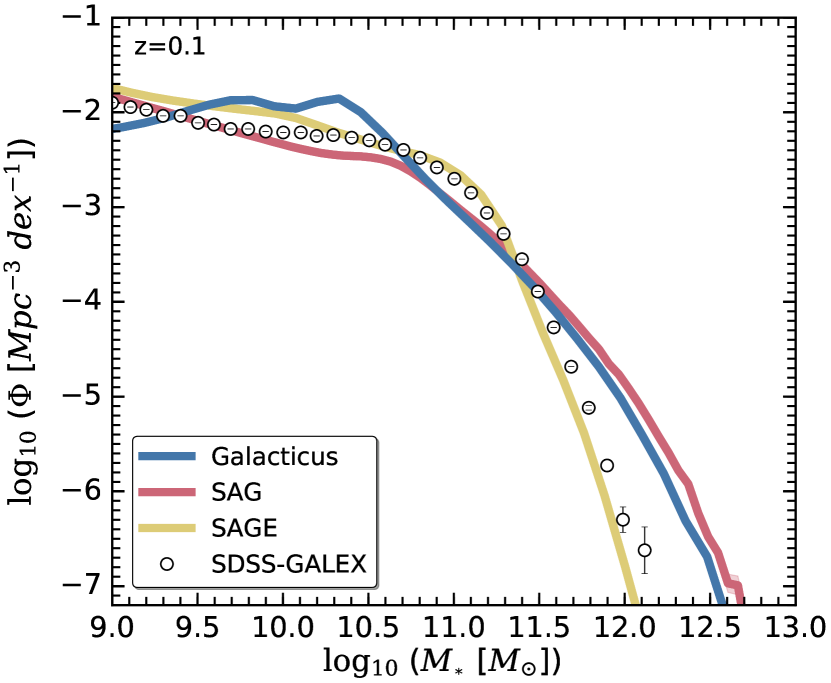
Figure 1: Stellar mass function of all three models in comparison with the SDSS-GALEX observation at $z=0.1$

One of the most fundamental properties of galaxies is the stellar mass and its distribution into individual galaxies, as measured by the galaxy stellar mass function (SMF). Generally, SMFs also play a central role for the calibration of the models, i.e. model parameters are fine-tuned to reproduce a given observationally measured SMF.

In Fig. 1 we compare each of the three SAMs to the stellar mass function of the SDSS-GALEX survey at redshift $z=0.1$ (Moustakas et al., 2013). We observe a similar yet smaller model-to-model variation as already reported by Knebe et al. (2015): all models presented here provide a valid reproduction of the observed stellar mass function, but all with individual features, e.g. Galacticus shows a ‘bump’ at medium masses – a feature that will affect some of the other results shown below – and a flattening at smaller masses. Sage provides the closest match to the observational data. This is unsurprising given it is the strongest constraint used for that model, even though they did not use the observational data shown here, but Baldry et al. (2008) instead. However, both Galacticus and Sag over-predict galaxies at the very high-mass end. Croton et al. (2006) and Bower et al. (2006) relate such an excess to a radio-mode AGN feedback not being efficient enough to suppress star formation in these massive galaxies (see also Hirschmann et al., 2016). However, this has also been investigated in more detail with the Sag model here, but changing some aspects of the AGN feedback to avoid the excess at the high-mass end of the SMF did not lead to an improvement: when calibrating the code, the values of the free parameters change to compensate for those modifications, and the results are eventually the same. But we need to remind the reader that Sag simultaneously calibrates to the SMF at redshift $z=0$ and $z=2$ (cf. Table 1). And this is non-trivial for any SAM model (Henriques et al., 2014; Hirschmann et al., 2016; Rodrigues et al., 2017, Knebe et al., in prep., Asquith et al., in prep.). We also like to mention at this point that the excess of massive galaxies for Sag and Galacticus is not readily explained by a too high star formation rate – at least not when considering the local star formation rate function (see Section 3.2.1 below) where we find that all models reproduce the observed SFRF sufficiently well. This is further supported by aforementioned agreement of the SMF at $z=2$ with observational data and abrupt decay of SFR from $z=2$ for galaxies with masses larger than $10^{11}$$h^{-1}{\rm{M_{\odot}}}$ (Cora et al., in prep.).

We conclude that the results seen here in Fig. 1 have to be attributed to other aspects such as mergers or the treatment of orphans (see Section 2.5). In particular, one of the features of Sage is to tidally disrupt satellite galaxies when they become orphans adding their stars to the intra-cluster light. As Sage keeps track of this component, we confirm that adding it back to the mass of the galaxy substantially lifts the SMF for masses $\log_{10}(M_{*})>11.3$, i.e. above the knee (not shown here though), to a level where it is approximately 1.5dex larger than the other two models at $\log_{10}(M_{*})>12.5$. This exercise hints at possible inefficiencies in the mechanism of tidal stripping implemented in Sag. This process removes stellar mass from the disc and bulge of satellite galaxies that is deposited in the intra-cluster component. However, it seems that the stripped mass is being underpredicted, preventing tidal stripping from alleviating the discrepancy between model and observations at the high mass end of the SMF at $z=0$. This will be discussed in more detail in an accompanying paper that focuses on the treatment of orphan galaxies in the Sag model (Vega-Mart nez et al., in prep.).

3.2 Star Formation

While a fraction of the galaxy mass is expected to be ejected by stellar winds and new mass being accreted via mergers, different amounts of stellar mass across semi-analytic models – as found in the previous sub-section – also has to relate to different star formation rates (SFRs) and star formation histories, respectively. We investigate such differences in star formation across our models in this sub-section and compare them to observational data, too.

3.2.1 The Star Formation Rate Function (SFRF)

We start with showing in Fig. 2 the star formation rate function (SFRF), i.e. the number of galaxies per unit volume with a given SFR. The models are contrasted to observations from Gruppioni et al. (2015) who determined the SFR function in the redshift interval $z\in[0.0,0.3]$ whereas the SAM data are shown for redshift $z=0.14$. We find that all models reproduce it rather well although we again observe some scatter from model to model (bearing in mind that Sag used the SFRF as a constraint during parameter calibration). We further note that Galacticus and Sag have more galaxies with higher SFR as compared to Sage. They nevertheless both match the observational data and hence – as mentioned before – the SFR alone does not explain their excess of high-mass galaxies seen in Fig. 1, i.e. they form stars at the correct (i.e. observed) rate – at least during the epoch $0.0<z<0.3$ which is the redshift range of the observational data shown in Fig. 2. Their overabundance of high-mass galaxies as previously seen in Fig. 1 must be related to other phenomena as already discussed before.

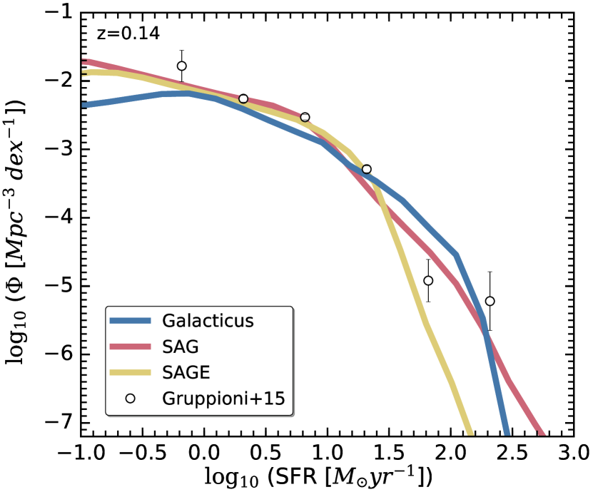
Figure 2: Star formation rate function for of all three models at $z=0.14$ compared to observations from Gruppioni et al. (2015).

3.2.2 The Specific Star Formation Rate to Stellar Mass Relation

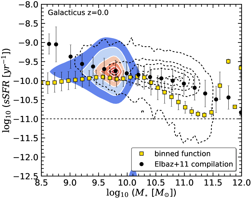
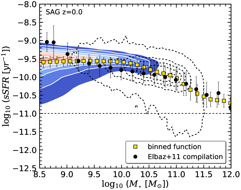
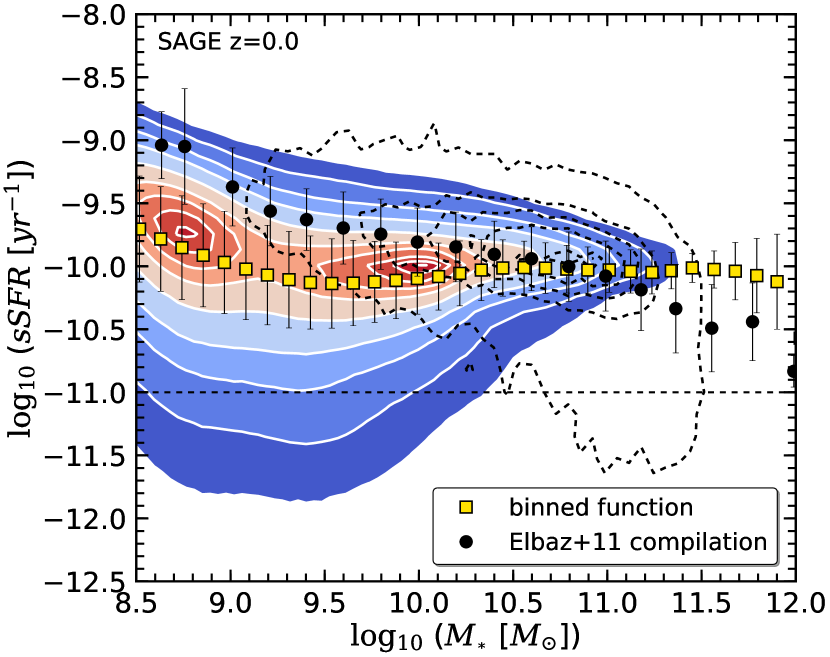
Figure 3: The specific star formation rate vs. stellar mass contours (coloured with white lines) and binned function for star-forming galaxies (yellow squares) at $z=0$ for Galacticus (top panel), Sag (middle panel) and Sage (bottom panel). As a reference we include a compilation of observations of star-forming galaxies (Elbaz et al., 2011, left panel of Fig. 16) which is presented here as dashed black contours as well as the a binned function (black dots) at $z\sim 0$. The dashed black line represents a commonly used separation of active and passive galaxies $\log_{10}(sSFR~{}[yr^{-1}])>\log_{10}(0.3/t_{Hubble(z=0)}[yr^{-1}])~{}\sim~{}-11$ (Franx et al., 2008).

Not all galaxies form stars at the same rate and the SFR certainly depends on the actual (stellar) mass of the galaxy. Thus, it is instructive to have a closer look at the specific SFR (sSFR), i.e. the star formation rate per unit stellar mass. Assuming a constant star formation rate, we like to remark that the inverse of the sSFR can serve as a proxy for galaxy age. We show sSFR vs. stellar mass as a contour plot (coloured with white lines) for our models at $z=0$ in Fig. 3. The dashed black line represents a commonly used separation of active and passive galaxies $\log_{10}(sSFR~{}[yr^{-1}])>\log_{10}(0.3/t_{Hubble(z=0)}[yr^{-1}])~{}\sim~{}-11$ (Franx et al., 2008). From this sample we calculate the binned function of active galaxies for our models, represented as yellow squares in the figure. We compare the model results to a compilation of star-forming galaxies from Elbaz et al. (2011) at $z\sim 0$ presented here both as black dashed contour lines and binned data (black dots). Fig. 3 gives us wider insight into the galaxy stellar masses as compared to studying the SFRF (Fig. 2) only. While the SFRF agreed impressively well with observations in the range $1~{}<~{}\textsc{{SFR}}[{{{\rm{M_{\odot}}}}}yr^{-1}]~{}<~{}30$, the sSFR as a function of stellar mass shows that the distribution of star-formation across galaxies follows a marginally different mass-trend as found in observations (especially for Galacticus and Sage). When interpreting the panels we need to bear in mind that observations are likely incomplete at the low-mass end – a region where all models still provide data. But as the specific star formation can be viewed as a proxy for the (inverse of the) age of a galaxy, all models agree with the observations in the sense that more massive galaxies tend to be older – at least in terms of stellar ages – a phenomenon also referred to as down-sizing (e.g. Cowie et al., 1996; Neistein et al., 2006; Fontanot et al., 2009). However, this trend is not as pronounced for Sage as for the other models as the highest-mass galaxies in Sage are too star-forming. These galaxies also have discs that are relatively too massive and bulges that are relatively too low in mass (see Fig.6 in Stevens et al., 2016), something to be remembered when discussing the black hole–bulge mass relation below.

3.2.3 The Cosmic Star Formation Rate Function (cSFRD)

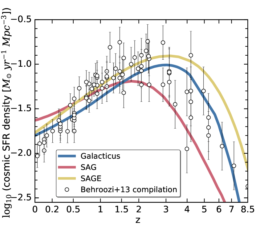
Figure 4: Cosmic star formation rate density for all galaxies as a function of redshift compared to a compilation of observations from Behroozi et al. (2013, Table 4).

In Fig. 4, we close this sub-section with a presentation of the evolution of the SFR density across cosmic time (cosmic star formation rate density, cSFRD), i.e. the so-called ‘Madau-Lilly plot’ (Lilly et al., 1996; Madau et al., 1996; Madau & Dickinson, 2014). We confirm that all three models show a pronounced peak around redshift $z\sim 2-3$ and approximately follow the observational data compiled by Behroozi et al. (2013) (shown here as open circles with error bars) within the error bars. However, their individual curves are rather distinct. Galacticus and Sage show approximately the same shape but appear shifted in amplitude with respect to each other, whereas Sag shows a marginally different shape. Up to redshift $z\sim 1$ (i.e. approximately 40 per cent of the present age of the Universe) the Sag model shows a substantially lower SFR. From that time onwards the model follows the same trend as Galacticus, albeit a marginally larger amplitude now. While Sag forms in total very few stars (due to the low SFR in the early Universe) it nevertheless provides roughly the same number of galaxies as Galacticus (see Table 2), especially above $\log_{10}({{M_{*}}}[{{{\rm{M_{\odot}}}}}])>10.5$ (see Fig. 1): that can be explained by the fact that there are lots of galaxies with low stellar mass, i.e. ${{M_{*}}}\leq 10^{8.5}$${\rm{M_{\odot}}}$ (not explicitly shown here, but can be concluded from the numbers in Table 2). And despite Sage having the highest integrated SFR the total number of galaxies is lowest for this model (see Table 2). Sage forms – in total – the fewest number of galaxies below ${{M_{*}}}<10^{8}$${\rm{M_{\odot}}}$ (as can be inferred again from Table 2, noting also that Sage does not feature orphans). Therefore the question remains why Sage – with reasonable matches to both the observed SFRF and SMF – shows a consistently higher cSFRD for redshifts $z>0.5$. While we leave a more detailed study of high-redshift galaxies to future work, we have seen – at least at redshift $z=0$ – that Sage features a marginal excess of sSFR as seen for high-mass galaxies in Fig. 3: for stellar masses $\log_{10}({{M_{*}}})>11$, Sage shows the highest sSFR amongst all models.

One can now raise the question about the interplay and simultaneous interpretation, respectively, of the four plots presented in this Section. For instance, the integral over all masses of the SMF at a fixed redshift corresponds to the integral of the cSFRD up to that redshift. Further, the integral over all SFR values in the SFRF gives the point in the cSFRD at the corresponding redshift. However, this relation has to be viewed with care because of the recycle fraction of exploding stars and/or produced by stellar winds which has to be considered during that integration. Fig. 4 now tells us that at redshift $z=0.14$ Sag has a higher (integrated) SFR than the Galacticus model. But when comparing this to Fig. 2 one needs to bear in mind that the excess seen there for Sag and Galacticus at the high-SFR end hardly contributes to such an integral. And the fact that the Sage  model gives the smallest number of galaxies (cf. Table 2) is also not inconsistent with the fact that its cSFRD is highest (at least for redshifts $z>0.5$): it simply means that all those stars generated over the course of the simulation are forming part of the lower mass galaxies (note that for stellar masses $\log_{10}{(M_{*}[{{{\rm{M_{\odot}}}}}])}<11.3$ Sage provides the highest SMF, cf. Fig. 1).

Therefore, while the set of plots presented in this Section clearly show consistency, they are not sufficient to explain, for instance, an excess of high-mass galaxies in the SMF plot. But it is apparent that for both Sag and Galacticus those objects with high SFR (as seen in Fig. 2) have to be high in stellar mass, too. Similarly, the deficit of objects with high SFR for Sage evidently helps the model to better reproduce the high-mass end of the SMF, even though those high-mass galaxies have rather high sSFR’s, according to Fig. 3. Further, for the Sag model we also confirm that galaxies with stellar mass $M_{*}<10^{11}$${\rm{M_{\odot}}}$ are actually responsible for the ‘excess’ seen in the cSFRD.

3.3 The Black Hole to Bulge Mass Relation (BHBM)

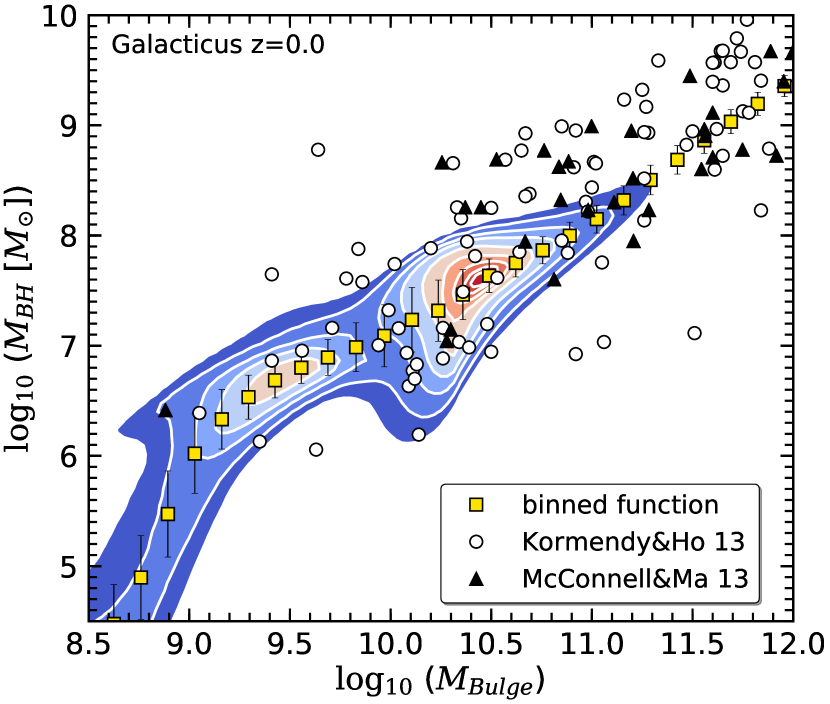
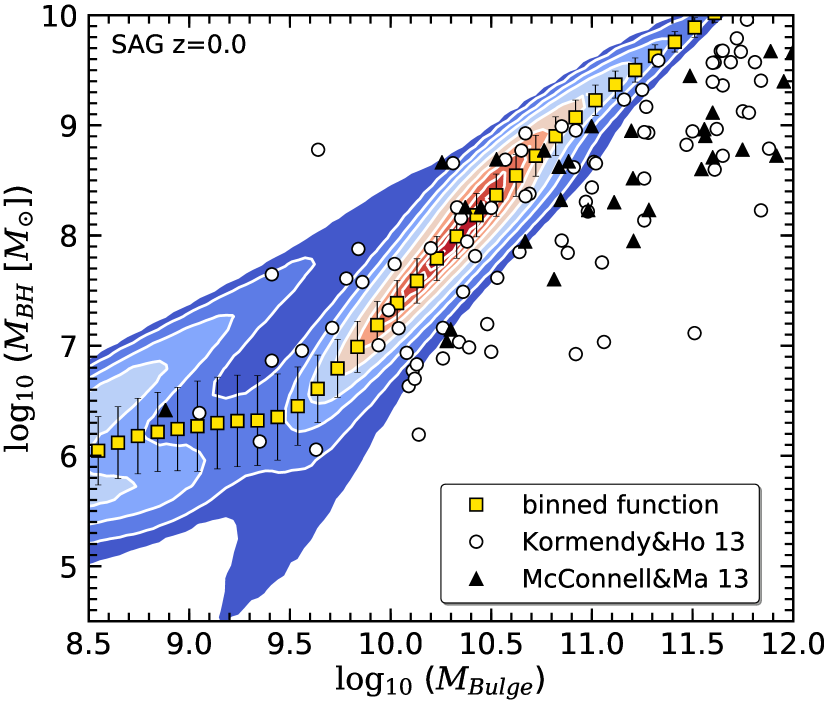
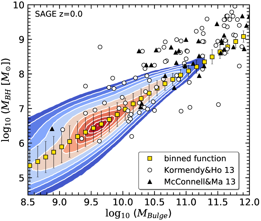
Figure 5: The contours show the relation of the black hole mass to stellar bulge mass at redshift $z=0$ compared to observations from Kormendy & Ho (2013) (open circles) and McConnell & Ma (2013) (filled triangles) for Galacticus (top panel), Sag (middle panel) and Sage (bottom panel). The yellow squares represent the binned data points of the same relation for a certain model.

It is very challenging to observe black hole (BH) masses in galaxies especially in a lower mass regime. Therefore SAMs provide a helpful and valuable tool to study possible correlations of galaxy properties – even at scales not yet well probed observationally. And black hole growth and growth in stellar mass are connected via feedback mechanisms (e.g. AGN feedback); therefore, BH growth plays a critical role in galaxy evolution (Croton et al., 2006; Bower et al., 2006; Croton et al., 2016). For more than a decade the picture that BHs and bulges co-evolve by regulating each others growth was mainly accepted. However, more recent studies support a more advanced picture claiming that BHs correlate differently with different galaxy components (Kormendy & Ho, 2013). In Fig. 5, we present the BHBM for Galacticus (top panel), Sag (middle panel) and Sage (bottom panel) at redshift $z=0$ as coloured contours and binned data points (yellow squares). All three models are in excellent agreement with the observations reported by Kormendy & Ho (2013) and McConnell & Ma (2013); they all favour the almost linear relation (in log-space, i.e. a power-law in linear-space) between black hole and stellar mass. We note that all our models are tuned to match the BHBM relation, and hence the agreement reported here is expected.

However, we observe for Sag that for large bulge masses, the black holes are more massive than in the other models. This is due to the restriction imposed on the high mass end of the SMF at $z=0$. The Sag model tries to avoid the excess in the high-mass end making the AGN feedback as effective as possible by large accretions onto BHs (high values of $f_{BH}$ in the related equations; see formula in Section 2.3) which leads to their high masses. However, despite this strong effect, model predictions do not satisfy this particular aspect of the observational constraint, indicating that other processes must be revised, like tidal stripping and disruption of satellites galaxies, since the dry mergers at low redshifts with massive satellites seem to produce the excess at the high mass end.

The reason why the correlation for Sage does not extend to larger bulge masses – as, for instance, Sag – relates back to what we have already noted in Fig. 3, i.e. the star-forming massive galaxies in Sage have discs that are relatively too massive and bulges that are relatively too low in mass. There are, therefore, fewer galaxies with massive bulges than expected, meaning there are fewer galaxies hosting massive black holes (because the model is constrained for the black hole and bulge masses to meet the observed trend). While a thorough treatment of disc evolution in an extension of Sage has been presented in Stevens et al. (2016), we leave the application of that particular model (Dark Sage) to MultiDark for future work.

3.4 The Cold Gas Fraction (CGF)

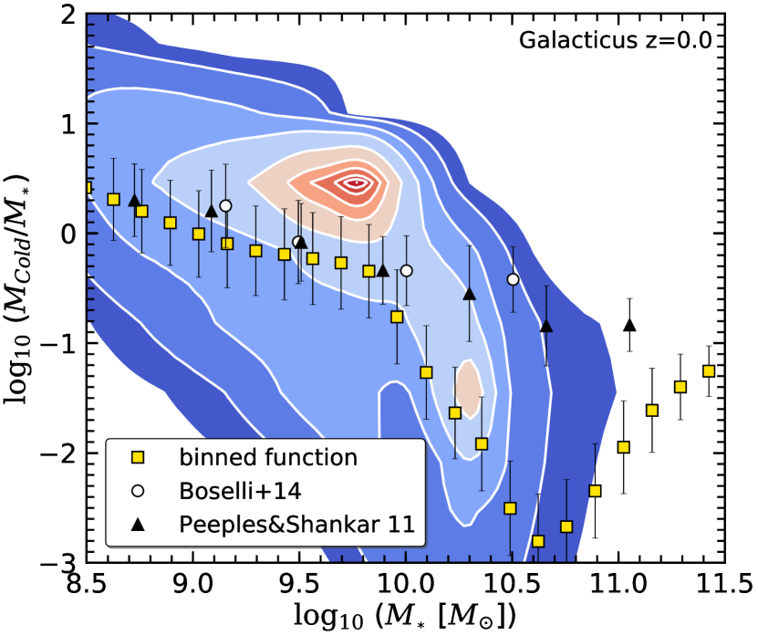
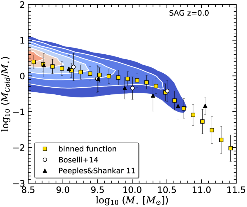
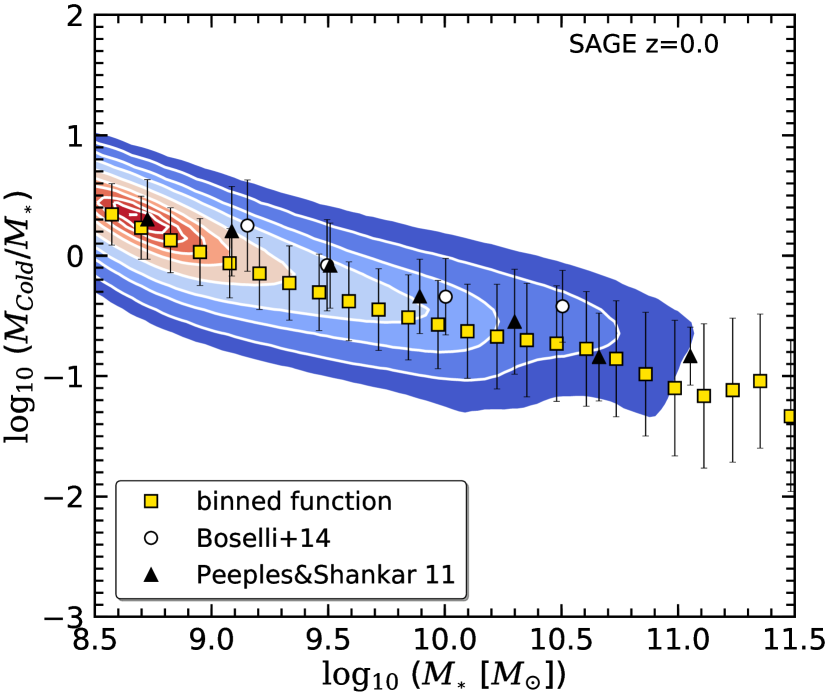
Figure 6: Fraction of cold gas compared to stellar mass as a function of stellar mass at redshift $z=0$ compared to observations from (Boselli et al., 2014, their Fig.5a) (open circles) and Peeples & Shankar (2011, Table 2) (black triangles). The yellow squares represent the binned data points of the same relation for a certain model.

An important tracer for star formation, age and metallicity is the fraction of cold gas to stellar mass. We therefore show in Fig. 6 the CGF vs. stellar mass for Galacticus (top panel), Sag (middle panel) and Sage (bottom panel) at redshift $z=0$ as coloured contours and binned data points (yellow squares). We report that Sag and Sage are in excellent agreement with the observational data points from Boselli et al. (2014, Fig.5a; open circles). This also applies to considering HI and CO detected late-type objects (Peeples & Shankar, 2011, compilation Table 2; black triangles) as well as considering HI from 21cm and HI+HII detected star-forming objects. Every data point of the binned function of Sage and Sag is located within the error bars of at least one of the observations, with the exception of Sag for $\log_{10}(M_{*}~{}[{{{\rm{M_{\odot}}}}}])~{}>11.0$. But note that Sag has been calibrated to the Boselli et al. (2014) data for which there are no data points beyond $\log_{10}(M_{*}~{}[{{{\rm{M_{\odot}}}}}])~{}>10.5$. Galacticus’ CGF drops rapidly between $10.0~{}<~{}\log_{10}(M_{*}~{}[{{{\rm{M_{\odot}}}}}])~{}<~{}11.0$. This is related to the current model of AGN feedback in Galacticus which is quite extreme, and dramatically reduces gas cooling above this scale. However, star formation rates remain high in these galaxies after AGN feedback kicks in, so they rapidly deplete their gas supply. However, we note that all our models are consistent with standard theories of star formation where massive, red galaxies either already used up their gas reservoir or (cold) gas became unavailable due to feedback mechanisms. Or – compared to the total stellar mass – they simply contain too small cold gas fractions (Lagos et al., 2014). All of this explains the low CGF for the high-$M_{*}$ galaxies see in this figure.

3.5 The Mass-Metallicity Relation

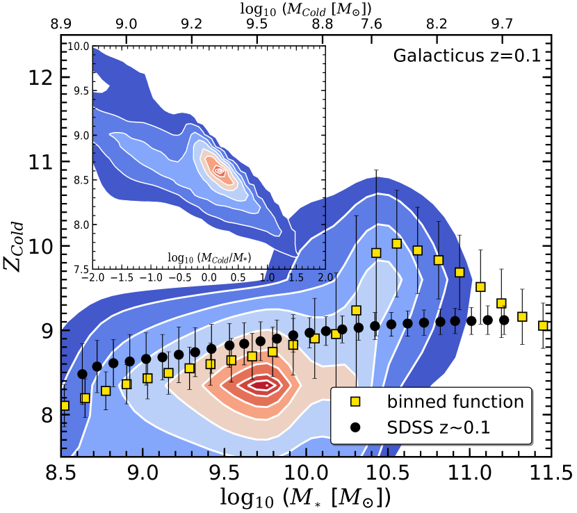
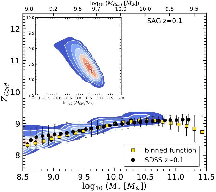
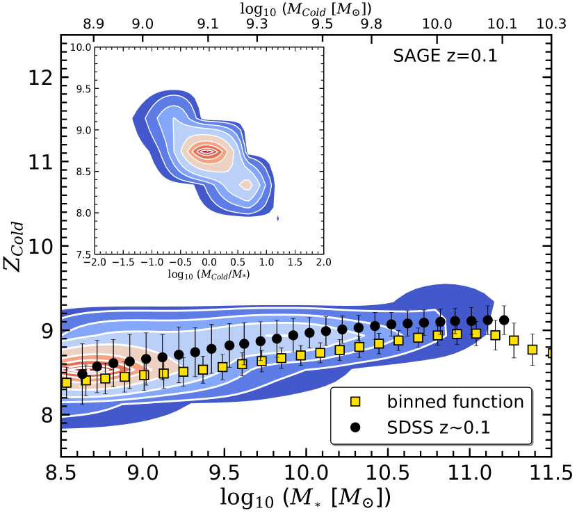
Figure 7: The total gas-phase metallicity to stellar mass relation at redshift $z=0.1$ compared to observations from Tremonti et al. (2004) (black dots error bars represent the 2.5/97.5 percentile of the distribution). The yellow squares represent the binned data points of the same relation for a certain model. The inset plot shows the same gas-phase metallicity as in the outer plot, but now compared to $M_{\rm cold}$/$M_{*}$.

Metals in galaxies are produced in stars and released into the inter-stellar and inter-galactic medium when stars let go of their gaseous envelopes or explode as supernovae. And as metals act as cooling agents in the process of star formation, their distribution throughout the galaxy also influences the (distribution of the) next generation of stars providing a link between metallicities and galaxy morphology (Lara-López et al., 2009a, 2010a; Yates et al., 2013). They are further strongly linked to stellar mass and star formation, leading to pronounced correlations with luminosities, and circular velocities as well.

We now verify such a relation between metallicity and stellar mass in the models by considering the total gas-phase abundance as a function of stellar mass using

$$Z_{\rm cold}=8.69+\log_{10}(M_{Z,\rm cold}/M_{\rm cold})-\log_{10}(Z_{\odot}),$$ (9)

where $M_{Z,\rm cold}$ is the mass of metals in the cold gas-phase and $M_{\rm cold}$ is the total gas mass. $Z_{\rm cold}$ is normalized by the metallicity of the Sun $Z_{\odot}=0.0134$ (Asplund et al., 2009), while the factor $8.69$ (Allende Prieto et al., 2001) corresponds to its oxygen abundance. Note that $Z_{\rm cold}$ as defined here is a conversion of cold gas metalicity to the oxygen abundance. Displaying metallicities this way is a commonly used approach in the literature, and hence it is also adopted here. Note that for Sage the total gas mass is given by the cold gas disc mass and that the other two models additionally provide a cold gas component for the bulge.

We present the results for the total gas-phase metallicity to stellar mass relation in Fig. 7. We find that the SAMs in general are in good agreement with the observational data from Tremonti et al. (2004). Compared to Fig. 6 where the $M_{\rm cold}$/$M_{*}$ ratio is decreasing, here the metallicity $Z_{\rm cold}$ is increasing with mass. That means that more massive galaxies tend to have a smaller cold gas reservoir and higher metallicity. The larger extent of the cold gas fraction seen in Fig. 6 for Galacticus is mirrored here again: for a fixed $M_{*}$ value, the spread in predicted metallicity is largest for Galacticus further hinting at a similar bimodality as for the cold gas fraction. The peak seen for this model at $\log_{10}(M_{*})\approx 10.5$ again relates to the depletion of gas due to the AGN feedback implementation in Galacticus: these galaxies have almost no inflow of pristine gas, and rapidly consume their gas supply. As expected from simple chemical evolution models the metallicity of the cold gas is driven up to the effective yield in this case. The other two models Sag and Sage show excellent agreement with the observational data – noting that this relation has been used during the parameter calibration for Sage. And the marginal offset seen for that model is simply due to the conversion from metal fraction to $Z_{\rm gas}$ being different for this plot versus the Sage calibration plot. To relate metallicity with cold gas mass we also include upper (approximated) tick marks representing the total cold gas mass $M_{\rm cold}$. Recent studies of the $M_{*}$-$Z_{\rm cold}$ relation suggest that there is an additional dependence of this relation on SFR (Ellison et al., 2008; Mannucci et al., 2010; Lara-López et al., 2009b, 2010b; Yates et al., 2012). Additional projections are used by various authors in their works including SFR and CGF to investigate the parameter space of these properties in more detail. The picture drawn by these works clearly corresponds to our current knowledge about galaxy formation. However, they report a ‘turnover’ towards low metallicities at low-$M_{\rm cold}$/$M_{*}$ (see Fig.6 in Yates et al., 2012) for galaxies with stellar masses $\log_{10}{({{M_{*}}}[{{{\rm{M_{\odot}}}}}])}\geq 10.5$. Since cold gas is the fuel for star formation – and metals are the required coolant – the gas-to-stellar mass ratio $M_{\rm cold}$/$M_{*}$, or equally $Z_{\rm cold}$, should correlate with the enrichment of the inter-stellar medium, hence metallicity of the gas. Yates et al. (2012) concluded that galaxies with low sSFR contribute to that turnover occurring at higher masses, in the sense that they tend to have lower ratio than other galaxies of a similar mass, caused by a gradual dilution of the gas phase in some galaxies. This is triggered by a gas-rich merger which shuts down subsequent star formation without impeding further cooling. They also drew a link between this ‘turnover’ and the black hole mass where they claim that these ‘turned-over’ galaxies also exhibit a larger central black hole mass. A detailed study inspired by Yates et al. (2012) would be interesting but beyond the scope of this paper. However, we here tested a few relations presented in their paper and can report a similar behaviour for our SAMs (see inset plots of Fig. 7). Furthermore, currently there is only limited observational data available to study this relation as well as its dependence on SFR, meaning that modelling metallicities will remain a very important tool and challenging task until sufficient data has been collected.

3.6 Stellar-to-Halo Mass Fraction (SHMF)

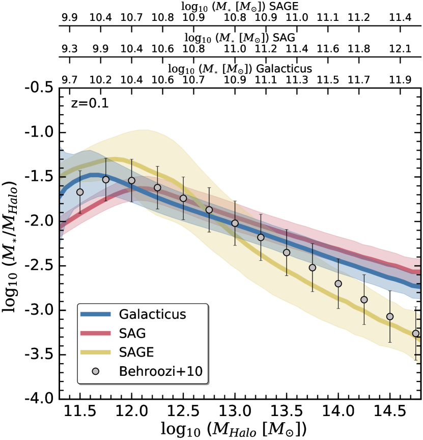
Figure 8: Stellar-to-halo mass ratio as a function of halo mass compared to the models of Behroozi et al. (2010) for non-orphan galaxies at $z=0.1$.

The previous sub-sections only dealt with the stellar and gas content of the galaxies (and its related properties). Here we draw a link to the dark-matter haloes they reside in. For this purpose we show in Fig. 8 the stellar-to-halo mass fraction $M_{\ast}/M_{\rm~{}Halo}$ (SHMF) as a function of dark-matter host mass $M_{\rm Halo}$. Note that we excluded orphan galaxies from this plot as they do not have an associated dark matter (sub-)halo any more by definition. Further, for satellite galaxies we assign the mass of their actual (sub-)halo to them and not the halo mass at the time of accretion to the encompassing dark matter host halo. Note that these two halo masses will be different as dark matter will be tidally stripped when orbiting within the overall host. We are aware that this will introduce a bias towards larger $M_{*}$/$M_{\rm Halo}$ values for satellite galaxies.

We compare our SAMs’ SHMF to the abundance matching model of Behroozi et al. (2010) at $z=0.1$. We report that our SAMs show a distinct peak around $\log_{10}{({{M_{\rm Halo}}}[{{{\rm{M_{\odot}}}}}])}\thicksim~{}12$, but slightly shifted either vertically or horizontally from the Behroozi data. The location of this peak as well as the slope of the SHMF provide deep insight into the physics of our models; the peak marks the halo mass for which the suppression of star formation changes from being controlled by AGN (higher halo mass) to domination of stellar feedback (lower halo masses). This peak should roughly coincide with the knee of the stellar mass function. To allow for such a comparison we provide in Fig. 8 as upper tickmarks an approximate conversion from halo to stellar mass, which is derived from a convolution of the SMF as presented in Fig. 1 with the stellar-to-halo mass ratio presented here. We note that all our models also agree with this expectation. The marginal excess at the high-$M_{\rm Halo}$ end for Galacticus and Sag is yet another reflection of the increased stellar masses at the high-mass end of the SMF: those galaxies – residing in the same dark-matter haloes as for Sage – have higher stellar masses than the corresponding galaxies in Sage.

3.7 Luminosity Functions (LF)

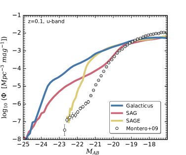
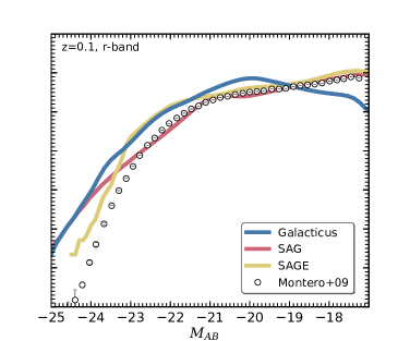
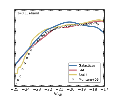
Figure 9: Luminosity function (rest-frame magnitudes) for the SDSS bands $u,r,i$ for the SAM models compared to observations from SDSS DR6 (Montero-Dorta & Prada, 2009).

Table 3: Stellar population synthesis (SPS) and dust (extinction) models applied to the SAMs in order to generate luminosities.

Model	SPS model	Dust Model	Provided Properties
Galacticus	Conroy et al. (2009)	Ferrara et al. (1999)	total luminosities
Sag	Bruzual & Charlot (2007)	observational constraints from Wang & Heckman (1996)	rest frame magnitudes AB-system
Sage	Bruzual & Charlot (2003)	Calzetti extinction curve (Calzetti, 1997, 2001)	rest frame magnitudes AB-system

We close the general presentation of the properties of our SAM galaxies with a closer look at luminosities. However, not all of the three models have returned luminosity-based properties as they introduce another layer of modelling, i.e. the employed stellar population synthesis (SPS) and dust model. In particular, the Sage model has not provided luminosities ab initio and they were modelled in post-processing via the Theoretical Astrophysical Observatory (TAO, Bernyk et al., 2016). This approach complies with the viewpoint of the Sage team: the majority of the computing time is spent on the construction of the primary galaxy catalogues, and the additional layer of SPS and dust is preferentially kept modular and separate from the rest of the SAM. The other two models directly returned either luminosities (Galacticus) or magnitudes (Sag) that have been uploaded to the database, whereas the reader should use TAO to generate Sage’s luminosities. An overview of their applied SPS used to create luminosities and dust extinction models can be found in Table 3. In what follows we describe how to unify the provided output and obtain rest-frame magnitudes for them, respectively.

Galacticus provides luminosities $L$ as an output (with the bandpass shifted to the emission rest-frame) which can be readily converted into flux densities $f$

$$f=L/4\pi D_{L}^{2}\ ,$$ (10)

where $D_{L}$ is the luminosity distance in $cm$. The resulting units of the flux density are $[ergs^{-1}cm^{-2}Hz^{-1}]$ and the zero-point flux density of the AB-System is given by $1~{}\text{ Jy}~{}=[10^{-23}ergs^{-1}cm^{-2}Hz^{-1}]$ (Oke & Gunn, 1983). We have to further apply a redshift correction factor to the flux to gain the correct fluxes in the frame of the filter. Using the standard equation to convert flux density into magnitudes in the AB-system and to calculate the magnitudes in the different SDSS ugriz bands we hence arrive at

$$m_{AB}=-2.5\log_{10}(f/3631\text{Jy})-2.5\log_{10}(1+z).$$ (11)

$m_{AB}$ are the magnitudes in the filter bands ugriz in the observed-frame. Note that these magnitudes correspond to the total galaxy luminosity and that also a dust correction has been applied (see Table 3). In order to calculate the absolute magnitudes in the rest-frame we have to substract the distance modulus and the K-correction to these magnitudes

$$M_{AB}=m_{AB}-DM-K_{cor}$$ (12)

where $DM=5\log_{10}(D_{L}/10\text{ pc})$ and $K_{cor}$ is the K-correction. The latter is calculated using the publicly available ‘K-corrections calculator’ (Chilingarian et al., 2010; Chilingarian & Zolotukhin, 2012).

The Sag model provides dust corrected absolute magnitudes in the rest-frame, therefore we do not need to apply any conversion.

As mentioned before, Sage’s magnitudes were calculated with TAO. This tool is a highly flexible and allows to select from a huge sample of filter band, SPS and dust extinction models to create magnitudes and colours for galaxies as a post-processing step separated from the actual simulation and galaxy creation. To generate magnitudes with TAO we used a subsample with 350 $h^{-1}\,{\rm Mpc}$ side-length and applied Chabrier IMF and the SPS and the dust extinction models presented in Table 3; we further only considered galaxies with stellar mass $M_{*}>1.46\times 10^{8}$.

We present the resulting luminosity function for the three SAMs in Fig. 9. The figure shows $LF$s in SDSS $u,r,i$ bands at $z=0.1$ compared to the observational data from Montero-Dorta & Prada (2009). Note that the observational data has been corrected to also give rest-frame luminosities allowing for an adequate comparison to our SAM data. While we find reasonable agreement at low-luminosities there are systematically too many bright galaxies for all three models, especially when considering the $u$-band. However, in the case of Galacticus and Sag this phenomenon is readily explained by the fact that for these two SAM models the SMF also shows an excess of high-mass galaxies: they contain too many stars, giving rise to too much light.

To gain more insight into this we present in Fig. 10 typical colour-magnitude and colour-stellar mass combinations at redshift $z=0.1$ for Galacticus (left column), Sag (middle column), and Sage (right column). In the top panel the SDSS rest-frame $u-r$ to the $r$-band relation is shown. The red dashed line corresponds to the commonly used separation of red and blue galaxies (Strateva et al., 2001). In the bottom panel we present the SDSS rest-frame $r-i$ to stellar mass relation.

Galacticus also shows a clear separation between a red and blue population as indicated by the reference line (dashed red) in the top panel as well as a reasonable colour-to-stellar mass relation. For Sag the top panel confirms what we already showed in Fig. 4; Sag shows a higher star formation rate than Galacticus for redshifts $z<1$, and hence the majority of galaxies is blue. However, this does not necessarily translate into a negligible red fraction: Sag also provides a reasonable red population, but due to the amount of lower mass blue galaxies (cf. bottom panel), its redder population is not resolved very well in these contour plots. We therefore include an inset panel for Sag when showing $r-i$ vs. stellar mass: in this representation – for which the same contour levels have been used, but the number density of galaxies is different due to applying a cut in stellar mass on the $x$-axis – the red population is clearly visible, too.

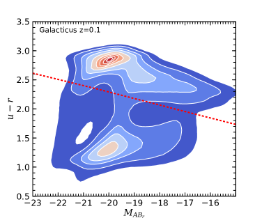
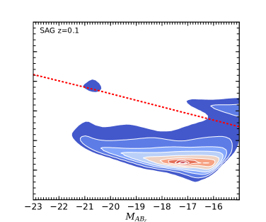
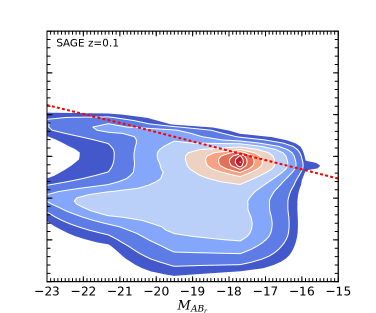
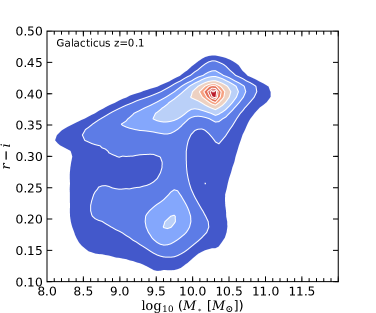
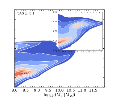
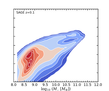
Figure 10: Colour-magnitude or colour-stellar mass diagrams in the rest-frame, respectively at redshift $z=0.1$ for Galacticus (left column), Sag (middle column) Sage (right column). Top: SDSS $u-r$ band to $r$-band relation. The dashed red line corresponds to the commonly used separation of red and blue galaxies (Strateva et al., 2001). Bottom: SDSS $r-i$ band to stellar mass relation.

4 Galaxy Clustering

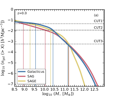
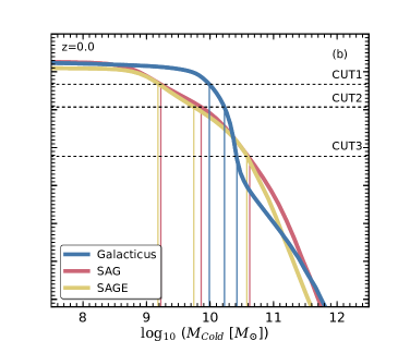
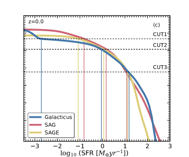
Figure 11: The cumulative abundance of SAM galaxies ranked by (a) $M_{*}$, (b) $M_{\rm cold}$ and (c) SFR. The vertical lines indicate how the applied number density cut translates into a lower limit for the respective galaxy property (see Table 4 for the actual values).

Table 4: Number density cuts for the selection of galaxy samples for the 2PCF calculation. The column labelled $X$ gives the translation of the number density cut into the corresponding cut in the respective galaxy property (i.e. $X$ can be $M_{*}$, $M_{\rm cold}$, or SFR).

CUT	$n_{\rm CUT}$	$X$	$\log_{10}(X_{\rm cut})$
	[($h^{-1}\,{\rm Mpc}$)3]		Galacticus	Sag	Sage
#1	46.75$\times 10^{-3}$	$M_{*}$	9.56	8.94	9.28
		$M_{\rm cold}$	9.99	9.23	9.18
		SFR	-2.71	-0.82	-1.08
#2	11.77$\times 10^{-3}$	$M_{*}$	10.43	10.04	10.31
		$M_{\rm cold}$	10.23	9.86	9.74
		SFR	-0.05	0.16	0.06
#3	0.53$\times 10^{-3}$	$M_{*}$	11.24	11.22	11.20
		$M_{\rm cold}$	10.42	10.62	10.58
		SFR	1.18	1.08	1.12

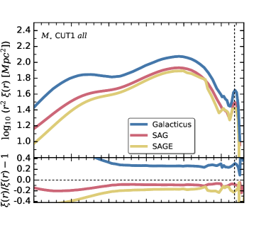
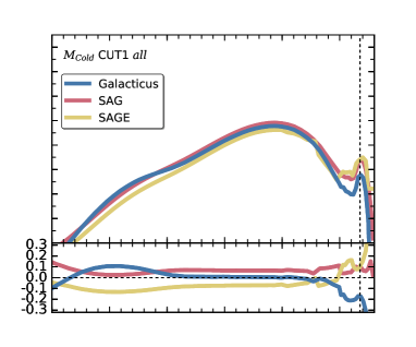
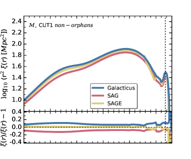
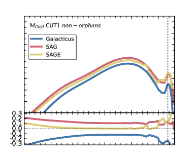
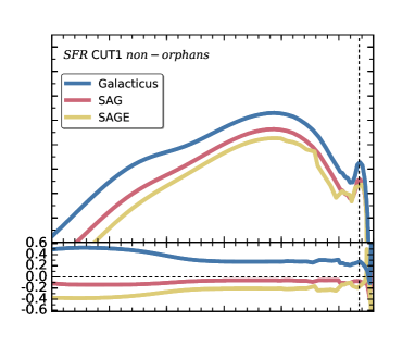
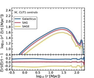
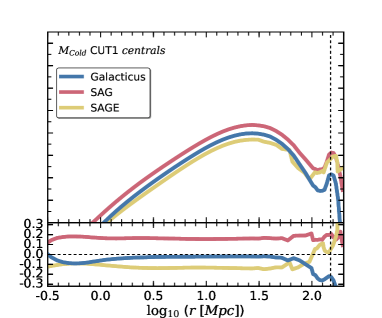
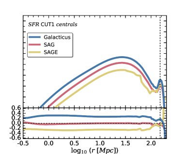
Figure 12: The real-space two-point correlation function at redshift $z=0.0$ for the density $CUT1$ ranked by the abundances of the following galaxy properties form left to right: $M_{*}$(left column), $M_{\rm cold}$ (middle column) and SFR (right column) and from top to bottom: ‘all’, ‘non-orphan’ and ‘central’ galaxies. The lower panel in each sub-plot shows the fractional difference with respects to the mean correlation function $\bar{\xi}(r)$. The vertical line indicates the position of the Baryonic Acoustic Oscillations peak. As Galacticus does not integrate the orbits of orphans, the positions of them correspond to the position of the central galaxy they orbit for that model. Sage does not feature orphans at all and hence the ‘all’ and ‘non-orphan’ curves are the same.

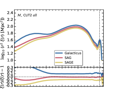
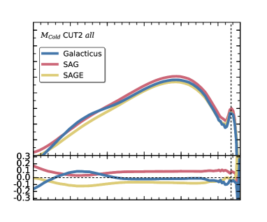
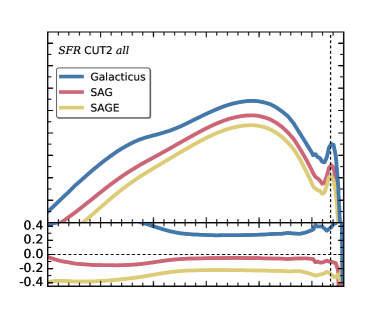
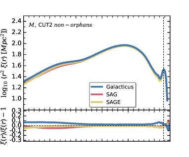
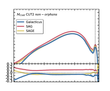
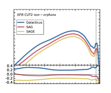
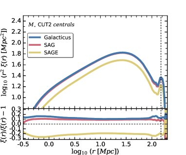
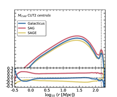
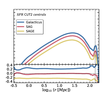
Figure 13: Same as Fig. 12, but for CUT2.

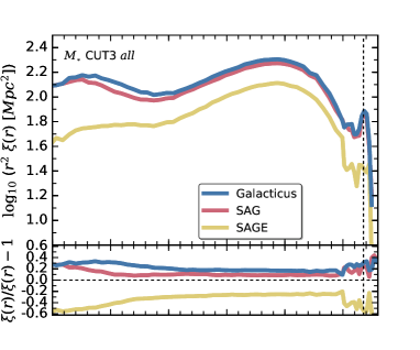
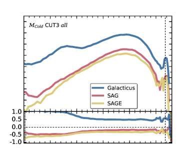
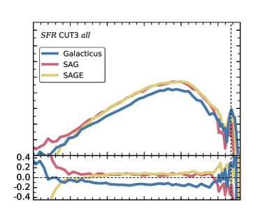
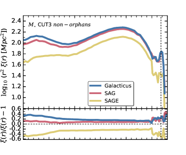
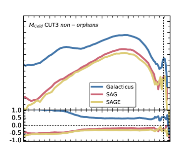
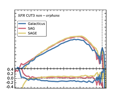
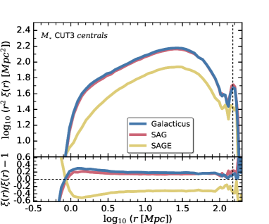
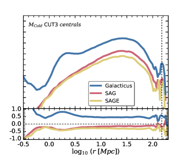
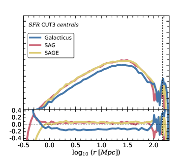
Figure 14: Same as Fig. 12, but for CUT3.

The spatial distribution of galaxies and their clustering properties in the matter density field carries an extensive amount of information, especially about cosmological parameters. Because of this, we are witnessing an ever-growing demand for mapping the three-dimensional distribution of galaxies across the sky and throughout the Universe through either ground-based (e.g. eBOSS, J-PAS, DES, HETDEX, DESI) or space-born (e.g. Euclid, WFIRST) missions. But the interpretation of those (redshift or photometric) galaxy surveys requires exquisite theoretical modelling. First and foremost, galaxies only serve as tracers of the underlying (dark) matter density field. And while galaxies do form within the potential wells of dark matter (e.g. White & Rees, 1978), their clustering amplitude cannot straightforwardly be related to the clustering amplitude of the matter density field due to the uncertainties in the bias relation. Further, individual surveys target only certain galaxies which introduces another level of bias and complexity.

In a recent work carried out as part of the ‘nIFTy Cosmology’ program we have presented a clustering comparison of 12 galaxy formation models, including variants of the SAM models presented here (Pujol et al., 2017). Like in the present study, all models were applied to the same halo catalogues and merger trees, but the sidelength of the cosmological box was only 62.5$h^{-1}\,{\rm Mpc}$ and hence probing galaxy clustering on much smaller scales. Contreras et al. (2013), on the other hand, used two different SAM models to study the two-point correlation function in the Millenium simulation. While both works found that the models generally agree in their clustering predictions, the observed differences for small scales reported in Pujol et al. (2017) can be attributed to orphan galaxies. Here we extend such a study by investigating the clustering properties on much larger scales. We will nevertheless put a focus on one of the prime differences between our three SAM models, i.e. the treatment of orphan galaxies. For the calculation of the 2PCFs we used the corrfunc software package. corrfunc is a set of high-performance routines to measure clustering statistics in a simulation box or on a mock catalogue (Sinha & Garrison, 2017). To calculate the correlation functions we are using always 60 log-spaced bins in the range of $0.1<r_{p}<200$ ${\rm Mpc}$ and in case of calculating the projected correlation function we integrate up to $\pi_{max}=60$ ${\rm Mpc}$.

For the calculation of the two-point correlation function (in real-space) we divide our galaxy catalogues into distinct galaxy sub-samples following the ideas of Contreras et al. (2013) by applying various cuts in number density. This initial idea of comparing catalogues from galaxy formation models at a fixed number density was developed by Berlind et al. (2003) and Zheng et al. (2005) within their analysis of a Halo-Occupation-Distribution (HOD) from hydrodynamical and semi-analytic models. By comparing the models at a fixed abundance, the authors were able to single out common features in their models. We are now choosing the same density cuts as given in Contreras et al. (2013) – who applied the same procedure – and listed here again in Table 4. Those cuts are applied to all our SAMs by using the

• cumulative stellar mass function,

• cumulative cold gas mass function, and

• cumulative star formation rate.

The respective distributions are shown in Fig. 11 and our applied cuts are illustrated as dashed lines. We like to remark that fixing the number density results in selecting galaxies for the three models with different cuts in the respective galaxy property. To better understand how the constant number density cut translates into the corresponding lower limit for the property in each model we show in Fig. 11 (as vertical lines) the intersection of the cumulative property distribution function with the applied number density cut. The resulting lower limits are additionally listed in Table 4.

Before calculating the two-point correlation functions we further sub-divided the ‘3 models $\times$ 3 CUTs’ roster of catalogues into three different galaxy populations: ‘all’ referring to the whole sample, ‘centrals’ restricting the calculation to central galaxies (i.e. galaxies residing at the centre of their main host halo, see definition in Fig. 16), and ‘non-orphans’ (i.e. galaxies with a host subhalo). Note, Sage does not feature orphans and hence the ‘all’ and ‘non-orphans’ sample are identical for this model. Further, Galacticus does not integrate the orbits of orphan galaxies but rather stores the position of dark matter halo at the time it was last found in the merger tree. While this makes their positions not suitable, in order not to loose the orphan galaxies and their contribution to at least the two-halo term of the correlation function we assign to them the position of the central galaxies of the halo they orbit in.

The clustering results for the three CUT samples is shown in Fig. 12 (CUT1), Fig. 13 (CUT2), and Fig. 14 (CUT3) as a 3$\times$3 grid on which the rows refer to ‘all’ (upper), ‘non-orphan’ (middle), and ‘central’ (lower) galaxies and the columns to cuts in $M_{*}$(left), $M_{\rm cold}$ (middle), and SFR (right). Each individual panel is further sub-divided into an upper part where we show the actual correlation function (multiplied by $r^{2}$ for clarity) and a lower part showing the fractional difference to the mean curve $\bar{\xi}(r)=\sum_{i=1}^{3}\xi_{i}(r)/3$ (summing over the three models). The vertical line indicates the position of the Baryonic Acoustic Oscillations peak (Beutler et al., 2011). In the following sub-section those figures will be discussed in the context of

• variations in number density, i.e. CUT1 vs. CUT2 vs. CUT3,

• changing galaxy property to define the sample, i.e. $M_{*}$ vs. $M_{\rm cold}$ vs. SFR,

• different galaxy populations, i.e. ‘all’ vs. ‘centrals’ vs. ‘non-orphans’

• model-to-model variations, i.e. Galacticus vs. Sag vs. Sage

4.1 Number Density Influence

As expected, we clearly observe that the correlation functions become more noisy when lowering the number density cut – especially on large scales. We also find that this introduces more disparity between the different models. For instance, the variations between Galacticus and Sag/Sage for $M_{\rm cold}$ non-orphans is minimal for CUT1/2, whereas it rises to 50 per cent when considering the CUT3 sample. As a matter of fact, the clustering continuously decreases for SFR-selected galaxies in Galacticus when lowering the threshold – whereas it remains rather constant for the other two models. For galaxies selected via a $M_{*}$-cut, we find that lowering the threshold increases the correlation on small scales. This is primarily driven by non-central galaxies for which the clustering on small scales naturally declines (see discussion in Section 4.3 below). The number density cuts have the smallest effect on Sag and Sage as well as galaxies selected via a SFR-cut: here we only observe a general increase of the noise level.

4.2 Galaxy Property Influence

We remind the reader that lowering the number density cuts for the $M_{*}$ selection basically means restricting the analysis to more massive galaxies, lowering in $M_{\rm cold}$ selects those with huge reservoirs of cold gas (i.e. galaxies with lower stellar mass according to Fig. 6), and lowering SFR corresponds to preferring star forming galaxies.

We observe that preferring star forming galaxies primarily affects the two-point correlation function due to a change in number density: the overall shape is preserved – at least on scales $r\mathrel{\hbox{\hbox to0.0pt{\hbox{\lower 4.0pt\hbox{$\sim$}}\hss}\hbox{$>$}}}1$${\rm Mpc}$. The largest effect is found when changing the $M_{*}$ number density cut. But this can be explained by the fact that more massive galaxies tend to be centrals and hence restricting the analysis to them will wash out any clustering signal on scales $r\mathrel{\hbox{\hbox to0.0pt{\hbox{\lower 4.0pt\hbox{$\sim$}}\hss}\hbox{$<$}}}1-2$${\rm Mpc}$, which is where the effect is observed to be strongest.

4.3 Galaxy Population Influence

The difference between the three populations is that ‘centrals’ limit the analysis to those galaxies that reside at the centre of a distinct dark-matter host halo, i.e. a halo that itself is not a subhalo of any larger object. For this sample, we do not expect a strong clustering signal on scale $r$$\;\buildrel<\over{\sim}\;$1–2${\rm Mpc}$ which corresponds to the size of these objects. The ‘non-orphans’ are a class of galaxies that do have a dark-matter host (sub-)halo which itself could be a distinct halo or a subhalo. Restricting the analysis to such objects comes closest to methods where dark matter halo catalogues are populated with galaxies by means of, for instance, halo abundance matching (HAM) as presented in the recent study by Rodríguez-Torres et al. (2016) for the BOSS galaxy clustering. The ‘all’ sample now covers all galaxies for which positional information is available, and that might include orphan galaxies (only for Sag though).

The main observation for changes in the galaxy population is the division of the clustering signal into a contribution from scales larger than the typical size of dark matter haloes and correlations inside those haloes, i.e. the decomposition into the so-called two- and one-halo term. We find that ‘non-orphans’ show correlations below $r$$\;\buildrel<\over{\sim}\;$1${\rm Mpc}$ whereas this is suppressed for ‘centrals’, especially for the CUT3 sample.

4.4 SAM Model Influence

We like to restate that one of the obvious differences between the models is the treatment of orphan galaxies: Galacticus provides physical properties for orphan galaxies (like masses, star formation rates, luminosities, etc.), but does not integrate the orbits; we therefore assigned the position of the central galaxy they orbit to them. Sag follows the trajectories of orphans after their dark matter halo disappeared and hence gives full information; Sage does not provide any information on orphans at all.

We observe that differences between models only become apparent when lowering the threshold for the CUT. While the clustering signal in general follows the same shape with differences in the amplitude of order less than 20 per cent, it rises above that for CUT3. But the model-to-model variations also depend on the galaxy property used in the CUT-selection. For instance, the largest model-to-model variations are found for galaxies selected via the SFR-cut. Here we observe deviations larger than 20 per cent across all CUT samples. And the increase in model differences when lowering the $M_{*}$-threshold is just a reflection of the differences seen in the stellar mass function in Fig. 1. Galacticus and Sag have a very similar high-mass end of the SMF and also show comparable clustering properties for these objects (also see Fig. 11). Similar arguments can be used to explain the similarities and differences seen across the other CUT properties $M_{\rm cold}$ and SFR: models showing correspondence in these (distributions of) properties are also alike when it comes to the clustering signal.

A lot of the differences seen in the 2PCF across models for various CUTs can also be attributed to the fact that keeping the number density constant leads to differing cuts in the respective galaxy property. This is readily verified in Fig. 11 where it can be seen that, for instance, CUT1 selects galaxies from the Galacticus catalogue with $M_{*}$$>10^{10}{{{\rm{M_{\odot}}}}}$ ($M_{\rm cold}$ $>10^{10}{{{\rm{M_{\odot}}}}}$) whereas this mass limit is $M_{*}$$>10^{9}{{{\rm{M_{\odot}}}}}$ ($M_{\rm cold}$ $>10^{9.3}{{{\rm{M_{\odot}}}}}$) for Sag. But we conclude that the shape of the 2PCF remains largely the same for the models and hence appears to be independent of the implementation of the physical processes.

4.5 Comparison to SDSS main galaxies

We close the presentation of the clustering statistics with a comparison of our model projected 2PCF (p2PCF) to different samples drawn from the SDSS DR7 main galaxy sample (Strauss et al., 2002). To this extent, we selected SAM galaxy samples within the following four absolute $r$-band magnitude bins

• $M_{r}\in[-19,-18]$,

• $M_{r}\in[-20,-19]$,

• $M_{r}\in[-21,-20]$, and

• $M_{r}\in[-22,-21]$.

Note that the samples are only selected by $r$-band magnitude and no additional cuts have been made.

As for the real-space correlation function we used the corrfunc Python package and compute the projected correlation function by choosing an integration length of $\pi_{max}=60$ ${\rm Mpc}$. We also tested if a different integration length would change our results, but cannot report any relevant differences when using $\pi_{max}=[40,80,100]$ ${\rm Mpc}$.

Our results can be viewed in Fig. 15 where show the p2PCF for the aforementioned four magnitude bins. In each of the panels we further compare them to the SDSS results from Zehavi et al. (2011, Table 7) at $z\sim 0.1$, within the same magnitude bins. The upper part of each panel shows the correlation function with the observations as open circles and the lower part represents the residuals with respect to the observations in the respective magnitude bin. In Table 5 we show the number densities and the fraction of satellites and orphan satellites, respectively, of our samples presented in Fig. 15.

All our models reproduce the basic features of the observational p2PCF, and the transition from the one-halo to the two-halo term at around $r_{p}\sim$1-2 ${\rm Mpc}$ is well described. Especially in the bin (a) where Sag and Sage reproduce the SDSS clustering signal perfectly for large separations, and in (b) where Galacticus describes the observational data best, and within 15-40 per cent. This can be understood if we take a look at the fraction of satellites in Table 5. Galacticus shows the largest fraction of satellites – when combining satellites and orphans together – and the largest fraction of orphans, respectively. As we discussed in previous sections, this again confirms how strong the clustering behaviour correlates with the galaxy type (see Figs. 12-14): models (in our case Sag and Sage) with smaller satellite fraction lack clustering power on small scales, but nevertheless reproduce the observed p2PCF very well beyond the one-halo term. However, we also need to remind the reader that the positions for the orphans in Galacticus coincide with the position of the central galaxy as that model does not integrate the orbits of satellite galaxies once they are stripped off their dark matter halo. And this artificially enhances the clustering signal. But it is remarkable to note that Sage – the model without any orphans – basically provides identical results to Sag – the model with the most sophisticated treatment of orphan positions. However, we also need to acknowledge that our cuts in magnitude introduce a selection-bias: we have seen in the upper panels of Fig. 10 that while all models feature red and blue galaxies, their exact locii in the colour-magnitude diagram are shifted with respects to each other. Therefore, using fixed bins in magnitude will select different populations.

If we consider the brighter magnitude end, as shown in panels (c) and (d), the clustering signals of the models are almost fully in agreement with each other. However, Galacticus always shows the largest clustering strength as seen before in panels (a) and (b). But for all of the SAM models the p2PCF is shifted downwards in amplitude about 50-80 per cent across the whole separation range.

Table 5: Number density measured in ($h^{-1}\,{\rm Mpc}$)^-3, for the selection of galaxy samples for the projected 2PCF calculation and the fractions of satellite and orphan satellites, respectively, in the four distinct magnitude bins used for Fig. 15.

panel
$M_{r}$ bin		Galacticus	Sag	Sage
(a)	$n_{\rm gal}$	12.22$\times 10^{-3}$	17.39$\times 10^{-3}$	18.86$\times 10^{-3}$
$[-19,-18]$	fsats	0.11	0.15	0.12
	forphans	0.58	0.09	-
(b)	$n_{\rm gal}$	20.34$\times 10^{-3}$	10.65$\times 10^{-3}$	15.39$\times 10^{-3}$
$[-20,-19]$	fsats	0.18	0.16	0.15
	forphans	0.28	0.05	-
(c)	$n_{\rm gal}$	17.36$\times 10^{-3}$	8.07$\times 10^{-3}$	11.10$\times 10^{-3}$
$[-21,-20]$	fsats	0.17	0.17	0.15
	forphans	0.10	0.03	-
(d)	$n_{\rm gal}$	6.48$\times 10^{-3}$	3.49$\times 10^{-3}$	10.01$\times 10^{-3}$
$[-22,-21]$	fsats	0.17	0.12	0.13
	forphans	0.03	0.02	-

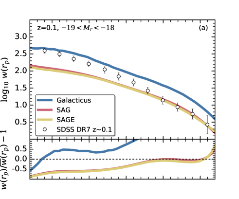
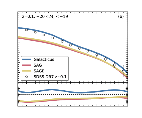
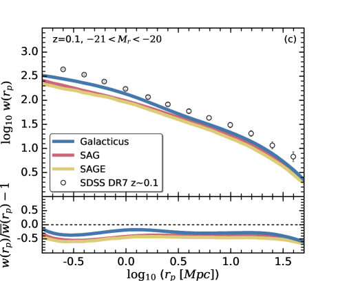
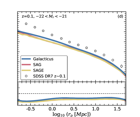
Figure 15: The projected 2PCF for different $r$-band abslute magnitude $M_{r}$ bins compared to SDSS DR7 observations in the same bins taken from Zehavi et al. (2011). The bottom panels are again the fractional difference with respect to the mean $\bar{w}(r_{p})$ (defined in the same way as for Fig. 12).

5 Summary and Discussion

We present the public data release of three distinct galaxy catalogues from the three semi-analytic models Galacticus, Sag, and Sage as applied to the same underlying cosmological dark-matter simulation MDPL2. The two latter models Sag and Sage have been re-calibrated to the simulation whereas Galacticus has been used with its standard choice for the parameters. In the first part of the paper, we compared the model galaxies to observational data. This serves as a gauge for the performance of the models. Even though the general aim of each SAM is to model galaxy formation, it is important to bear in mind that models might be tuned to serve different purposes. Therefore, our three models perform differently as they put their focus differently: Sage fits multiple observables simultaneously, first and foremost the stellar mass function and stellar-to-halo mass relation; Galacticus has its strength in the star formation rate function and evolution; and Sag is a model with strengths in providing reasonable gas fractions and metallicity relations. Further, the most recent changes implemented into the Sag model (cf. Section 2.3) produce galaxies with properties in excellent agreement with observations such as the galaxy main sequence (sSFR vs. stellar mass, Fig. 3) and the mass-metallicity relation (Fig. 7), yet showing an excess of galaxies at the high-mass end of the SMF at redshift $z=0$. These ‘model priorities’ are certainly reflected by the plots presented in Section 2.3. We have seen that Sag fits the sSFR-$M_{*}$ relation of Elbaz et al. (2011) much better than both Galacticus and Sage, Galacticus fits the cosmic SFR density at low-$z$ better than the other two SAMs, but it does it because its under-efficient star formation (low sSFR) is compensated by an excessive stellar mass density, and Sage fits the SDSS+GALEX data much better than Galacticus and Sag. We relate the latter to the distinct treatment of orphans in Sage. This model does not feature any galaxies devoid of a dark matter halo but rather disrupts them adding their stars to an intra-cluster component. While both other models treat such a component differently, it furnishes Sage with the possibility to deposit stars that in the other two models find their way into the galaxies and hence leading to a larger stellar mass than for Sage. And while Sag also features such a component, the implementation of tidal stripping appears to be too inefficient and hence leading to an under-estimated stellar content in its ICC. While this difference cannot explain all of the deviations seen at the high-$M_{*}$ end in the SMF plot Fig. 1 it certainly plays a significant role. For all these reasons of different model designs, we considered it important to have not only a single but multiple galaxy formation models available exploring different approaches to galaxy formation physics.

In the second part of the paper we applied three galaxy number density cuts in stellar mass, cold gas fraction, and star formation rate to define various sub-samples of galaxies for a study of the two-point correlation function. We confirm the results recently reported by Pujol et al. (2017), i.e. even though there might be noteworthy variations of internal properties of galaxies across different SAMs, the positions are stable and there is only very little scatter in the clustering properties of our galaxies – irrespective of the selection criterion for the chosen sub-sample. The 2PCF shape largely remains the same across all models (at least on scales $\lower 2.15277pt\hbox{$\;\buildrel>\over{\sim}\;$}1$${\rm Mpc}$) and hence appears to be independent of the implementation of the physical processes. However, its amplitude (and thus any measurement of the galaxy bias) is affected. We further confirm that all our models reproduce the observed projected 2PCF albeit again showing model-to-model variations. This might again be attributed to variations in the treatment of orphan galaxies and number densities of galaxies in the respective magnitude bin, but also relates to the fact that the applied magnitude cuts introduce a selection bias.

We conclude that the models applied here and the galaxy catalogues based upon them will be a valuable asset to the community and can be readily used for science that requires reliable galaxy information in volumes large enough to match on-going and upcoming surveys. And unless SAM models are specifically designed to predict (and/or describe) the same galaxy properties, physical processes are treated identically, and calibration has been performed in an identical manner, model-to-model variations as seen here are expected (Lee et al., 2014; Knebe et al., 2015, Knebe et al., in prep.): models perform differently reflecting their individual designs. Therefore, it appears important to not only regard a single model but a selection of models when studying mock galaxies in order to properly capture such scatter. However, one might argue that a better approach would be to fine-tune each model to the actual simulation until the observations used in that calibration procedure are best reproduced. But this becomes intrinsically difficult the larger the simulations are and sub-sets have to be used for the parameter adjustment. Further, even a scrupulous re-calibration will not guarantee that different galaxy formation models will all give the same results (see Knebe et al., in prep.). To achieve perfect agreement a universal protocol would need to be defined that involves using the same observational data sets, the same allowance for scatter during the calibration, the same assumption for initial mass functions, the same yields, the same recycled fractions, etc. But in the end differing implementations of the same physics will eventually leave us with some level of residual variance (e.g. Fontanot et al., 2009; Lu et al., 2014).

We close with the remark that this paper only forms the first in a series where the models and their galaxies will be studied in far more detail. This paper simply introduces the three galaxy catalogues (Galacticus, Sag, and Sage) populating a common dark matter simulation (MDPL2) that is large enough to tackle cosmological questions such as the position and width of the Baryon Acoustic Oscillation peak and how this is affected by baryon physics. Besides of publicly releasing all data, the source code of two of the galaxy models (Galacticus and Sage) is open too, allowing the community to explore the impact that the specific modelling of a physical process has on different measurements used in cosmology, open the possibility to also explore the cross correlation of different cosmological tracers

Appendix A Database Release

All the data used for this paper are publicly available. While we refer to Section 2.1 for a description of the simulation, halo catalogues, and merger trees, we like to present here some of the particulars of the galaxy catalogues. The data can be individually referenced by using a Digital Object Identifier (DOI): we list them in Table 6 for the three models in the database.

Galacticus has been run in its native configuration, whereas Sag and Sage retuned their parameters to the MDPL2 simulation. In Table 7 we list those properties that are common to all models and for which we chose identical names in the database. Those properties have also been converted to the same units. For Galacticus and Sag luminosities/magnitudes have also been uploaded to the database whereas for Sage they have to be generated by the user on TAO. We further encourage the reader to visit the database website and the additional documentation provided there as the list of galaxy properties for each model is not limited to what is shown in Table 7: for each model substantially more information has been added to the database.

We further provide in Fig. 16 the nomenclature for the pointers to the haloes of the galaxies. A HostHaloID will point to the immediate dark matter host halo around the galaxy, which does not exist anymore for orphan galaxies by definition (but points to the last halo to which the galaxy belonged, i.e. a halo from a previous snapshot). The MainHaloID pointer will give access to the top-level dark matter halo in which the galaxy orbits while HaloID points to the lower-level halo around the galaxy. Note that HaloID=HostHaloID for all but orphan galaxies, and that HaloID only exists for Sag (which is why it is omitted from the list in Table 7).

Table 6: DOI’s for the three models.

catalogue	DOI
MDPL2-Galacticus	doi:10.17876/cosmosim/mdpl2/009
MDPL2-Sag	doi:10.17876/cosmosim/mdpl2/007
MDPL2-Sage	doi:10.17876/cosmosim/mdpl2/008

Table 7: Set of galaxy properties common to all semi-analytic galaxy formation models. For a sketch explaining the halo pointers please refer to Fig.1 of Knebe et al. (2015). Note that $x,y,z,v_{x},v_{y},v_{z}$ have been integrated for orphans in Sag yet are unavailable for Galacticus (the Sage model does not feature orphans). Please note that many more than the properties listed here have been uploaded to the database; please refer to the database website for more information.

database name	unit	description
redshift	n/a	redshift $z$
HostHaloID	n/a	pointer to dark matter halo in which galaxy resides;
		not applicable for orphan galaxies
MainHaloID	n/a	pointer to dark matter halo in which galaxy orbits
GalaxyType	n/a	0 = central galaxy
		1 = satellite galaxy
		2 = orphan galaxy (only for Galacticus and Sag)
X	comoving $h^{-1}\,{\rm Mpc}$	$x$-position of galaxy
Y	comoving $h^{-1}\,{\rm Mpc}$	$y$-position of galaxy
Z	comoving $h^{-1}\,{\rm Mpc}$	$z$-position of galaxy
Vx	peculiar km/s	$v_{x}$-velocity of galaxy
Vy	peculiar km/s	$v_{y}$-velocity of galaxy
Vz	peculiar km/s	$v_{z}$-velocity of galaxy
MstarSpheroid	$h^{-1}{\rm{M_{\odot}}}$	stellar mass of bulge component of galaxy
MstarDisk	$h^{-1}{\rm{M_{\odot}}}$	stellar mass of disc component of galaxy
McoldSpheroid	$h^{-1}{\rm{M_{\odot}}}$	cold gas mass of bulge component of galaxy
McoldDisk	$h^{-1}{\rm{M_{\odot}}}$	cold gas mass of disc component of galaxy
Mhot	$h^{-1}{\rm{M_{\odot}}}$	total hot gas mass in galaxy
Mbh	$h^{-1}{\rm{M_{\odot}}}$	mass of central black hole
SFR	$h^{-1}{\rm{M_{\odot}}}$/Gy	total star formation rate
SFRspheroid	$h^{-1}{\rm{M_{\odot}}}$/Gy	star formation rate in bulge component of galaxy
SFRdisk	$h^{-1}{\rm{M_{\odot}}}$/Gy	star formation rate in disc component of galaxy
MeanAgeStars	Gyrs	mean age of all stars
HaloMass	$h^{-1}{\rm{M_{\odot}}}$	$M_{\rm 200c}$ of galaxy’s dark matter halo
Vmax	km/s	peak circular rotation velocity of galaxy’s dark matter halo
Vpeak	km/s	maximum Vmax across all redshifts
NFWconcentration	n/a	concentration of galaxy’s dark matter halo
SpinParameter	n/a	spin parameter $\lambda$ of galaxy’s dark matter halo
MZstarSpheroid	$h^{-1}{\rm{M_{\odot}}}$	mass of metals in stellar component of bulge
MZstarDisk	$h^{-1}{\rm{M_{\odot}}}$	mass of metals in stellar component of disc
MZgasDisk	$h^{-1}{\rm{M_{\odot}}}$	mass of metals in gas component of disc
MZhotHalo	$h^{-1}{\rm{M_{\odot}}}$	mass of metals in hot gas component of halo
Galacticus luminosities and metalicities:
LstarSDSSu	$4.4659\times 10^{13}$ W/Hz	total stellar luminosity in SDSS u band
LstarSDSSg	$4.4659\times 10^{13}$ W/Hz	total stellar luminosity in SDSS g band
LstarSDSSr	$4.4659\times 10^{13}$ W/Hz	total stellar luminosity in SDSS r band
LstarSDSSi	$4.4659\times 10^{13}$ W/Hz	total stellar luminosity in SDSS i band
LstarSDSSz	$4.4659\times 10^{13}$ W/Hz	total stellar luminosity in SDSS z band
MZgasSpheroid	$h^{-1}{\rm{M_{\odot}}}$	mass of metals in gas component of bulge
Sag magnitudes and metalicities:
MagStarSDSSu	n/a	magnitude in SDSS u band
MagStarSDSSg	n/a	magnitude in SDSS g band
MagStarSDSSr	n/a	magnitude in SDSS r band
MagStarSDSSi	n/a	magnitude in SDSS i band
MagStarSDSSz	n/a	magnitude in SDSS z band
MZgasSpheroid	$h^{-1}{\rm{M_{\odot}}}$	mass of metals in gas component of bulge
Sage luminosities and metalicities:
- to be processed via TAO
- no additional metalicities

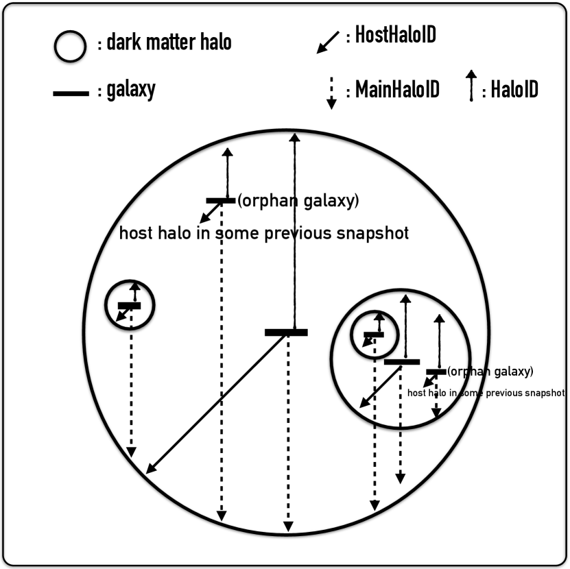
Figure 16: Illustrating the various pointers to haloes in which galaxies are residing.

Appendix B Summary of plots in Section 3

To facilitate the reading of Section 3 and provide more convenient access to the information about the data presented in this paper we summarize in Table 8 all the plots to be discussed in that Section. That table lists what galaxy property (or correlation between properties) is presented in which sub-section of the paper. It further indicates whether or not any selection criterion for our model galaxies has been applied. The following columns then provide information about the reference data used for each particular plot, i.e. the actual bibliographic reference, the redshift range of that data, the IMF entering into the derivation of that data.

Table 8: Here we provide a short description of the plots we present in Section 3. The first column ‘property’ corresponds to the physical or statistical property under investigation. The second column points to the ‘sub-section’ where the plot is discussed. The third column indicates whether we applied any cut to the data. The fourth column provides the reference for the observational data or other computations. The fifth and sixth column likewise give the redshift and IMF for the observational/reference data. If that reference data is not based upon a Chabrier (2003) IMF, we convert it.

property	sub-section	selection	reference	redshift	IMF
Stellar mass function	3.1	NO	SDSS-Galex	0.1	Chabrier (2003)
(SMF)			(Moustakas et al., 2013)
Star formation rate	3.2.1	NO	GOODS-S+COSMOS/PACS+	$0.0<z<0.3$	Chabrier (2003)
function (SFRF)			Herschel (Gruppioni et al., 2015)
Specific SFR to stellar	3.2.2	NO	Elbaz et al. (2011)	0.0	Salpeter (1955)
mass function
Cosmic star formation	3.2.3	sSFR	Behroozi et al. (2013)	$0.0<z<8.0$	Chabrier (2003)
rate density (cSFRD)		$>10^{-11}yr^{-1}$
Black hole to	3.3	NO	Kormendy & Ho (2013)	0.0	dynamical zero-point
bulge mass (BHBM)			McConnell & Ma (2013)	0.0	-
Cold gas fraction to	3.4	NO	Boselli et al. (2014)	0.0	Chabrier (2003)
stellar mass (CGF)			Peeples & Shankar (2011)	0.0	Chabrier (2003)
Total gas-phase metallicity	3.5	NO	Tremonti et al. (2004)	0.1	Kroupa (2001)
Stellar to halo mass	3.6	non-orphans	Behroozi et al. (2010)	0.1	Chabrier (2003)
function (SHMF)
Luminosity function (LF)	3.7	NO	SDSS (Montero-Dorta & Prada, 2009)	0.1	-
Colour diagrams	3.7	$M_{*}$	‘red’-‘blue’ separation	0.1	-
		$>1\times 10^{8}$ $[M_{\odot}]$	Strateva et al. (2001)

References

- Allende Prieto et al. (2001) Allende Prieto C., Lambert D. L., Asplund M., 2001, ApJ, 556, L63
- Asplund et al. (2009) Asplund M., Grevesse N., Sauval A. J., Scott P., 2009, ARA&A, 47, 481
- Avila et al. (2014) Avila S., Knebe A., Pearce F. R., Schneider A., Srisawat C., Thomas P. A., Behroozi P., Elahi P. J., Han J., Mao Y.-Y., Onions J., Rodriguez-Gomez V., Tweed D., 2014, MNRAS, 441, 3488
- Baldry et al. (2008) Baldry I. K., Glazebrook K., Driver S. P., 2008, MNRAS, 388, 945
- Baugh (2006) Baugh C. M., 2006, Rep. Prog. Phys., 69, 3101
- Begelman (2014) Begelman M. C., 2014, ArXiv e-prints
- Behroozi et al. (2015) Behroozi P., Knebe A., Pearce F. R., Elahi P., Han J., Lux H., Mao Y.-Y., Muldrew S. I., Potter D., Srisawat C., 2015, MNRAS, 454, 3020
- Behroozi et al. (2010) Behroozi P. S., Conroy C., Wechsler R. H., 2010, ApJ, 717, 379
- Behroozi et al. (2013) Behroozi P. S., Wechsler R. H., Conroy C., 2013, ApJ, 770, 57
- Behroozi et al. (2013) Behroozi P. S., Wechsler R. H., Wu H.-Y., 2013, ApJ, 762, 109
- Behroozi et al. (2013) Behroozi P. S., Wechsler R. H., Wu H.-Y., Busha M. T., Klypin A. A., Primack J. R., 2013, ApJ, 763, 18
- Benson (2010) Benson A. J., 2010, Phys. Rep., 495, 33
- Benson (2012) Benson A. J., 2012, New A, 17, 175
- Benson & Babul (2009) Benson A. J., Babul A., 2009, MNRAS, 397, 1302
- Benson et al. (2012) Benson A. J., Borgani S., De Lucia G., Boylan-Kolchin M., Monaco P., 2012, MNRAS, 419, 3590
- Benson & Bower (2011) Benson A. J., Bower R., 2011, MNRAS, 410, 2653
- Benson et al. (2000) Benson A. J., Cole S., Frenk C. S., Baugh C. M., Lacey C. G., 2000, MNRAS, 311, 793
- Berlind et al. (2003) Berlind A. A., Weinberg D. H., Benson A. J., Baugh C. M., Cole S., Davé R., Frenk C. S., Jenkins A., Katz N., Lacey C. G., 2003, ApJ, 593, 1
- Bernyk et al. (2016) Bernyk M., Croton D. J., Tonini C., Hodkinson L., Hassan A. H., Garel T., Duffy A. R., Mutch S. J., Poole G. B., Hegarty S., 2016, ApJS, 223, 9
- Bertschinger (1989) Bertschinger E., 1989, ApJ, 340, 666
- Beutler et al. (2011) Beutler F., Blake C., Colless M., Jones D. H., Staveley-Smith L., Campbell L., Parker Q., Saunders W., Watson F., 2011, MNRAS, 416, 3017
- Binney & Tremaine (1987) Binney J., Tremaine S., 1987, Galactic dynamics. Princeton, NJ, Princeton University Press, 1987, 747 p.
- Boselli et al. (2014) Boselli A., Cortese L., Boquien M., Boissier S., Catinella B., Lagos C., Saintonge A., 2014, A&A, 564, A66
- Bower et al. (2006) Bower R. G., Benson A. J., Malbon R., Helly J. C., Frenk C. S., Baugh C. M., Cole S., Lacey C. G., 2006, MNRAS, 370, 645
- Boylan-Kolchin et al. (2008) Boylan-Kolchin M., Ma C.-P., Quataert E., 2008, MNRAS, 383, 93
- Bruzual & Charlot (2003) Bruzual G., Charlot S., 2003, MNRAS, 344, 1000
- Bruzual & Charlot (2007) Bruzual G., Charlot S., 2007, private communication
- Bryan & Norman (1998) Bryan G. L., Norman M. L., 1998, ApJ, 495, 80
- Calzetti (1997) Calzetti D., 1997, in Waller W. H., ed., American Institute of Physics Conference Series Vol. 408 of American Institute of Physics Conference Series, UV opacity in nearby galaxies and application to distant galaxies. pp 403–412
- Calzetti (2001) Calzetti D., 2001, PASP, 113, 1449
- Chabrier (2003) Chabrier G., 2003, PASP, 115, 763
- Chilingarian et al. (2010) Chilingarian I. V., Melchior A.-L., Zolotukhin I. Y., 2010, MNRAS, 405, 1409
- Chilingarian & Zolotukhin (2012) Chilingarian I. V., Zolotukhin I. Y., 2012, MNRAS, 419, 1727
- Cole et al. (2001) Cole S., Norberg P., Baugh C. M., Frenk C. S., Bland-Hawthorn J., Bridges T., Cannon R., Colless M., Collins C., Couch W., Cross N., Dalton G., De Propris R., Driver S. P., 2001, Monthly Notices of the Royal Astronomical Society, 326, 255
- Comparat et al. (2017) Comparat J., Prada F., Yepes G., Klypin A., 2017, MNRAS, 469, 4157
- Conroy et al. (2009) Conroy C., Gunn J. E., White M., 2009, ApJ, 699, 486
- Contreras et al. (2013) Contreras C., Blake C., Poole G. B., Marin F., Brough S., Colless M., Couch W., Croom S., et al. 2013, MNRAS, 430, 924
- Cora (2006) Cora S. A., 2006, MNRAS, 368, 1540
- Cowie et al. (1996) Cowie L. L., Songaila A., Hu E. M., Cohen J. G., 1996, AJ, 112, 839
- Croton et al. (2006) Croton D. J., Springel V., White S. D. M., De Lucia G., Frenk C. S., Gao L., Jenkins A., Kauffmann G., Navarro J. F., Yoshida N., 2006, MNRAS, 365, 11
- Croton et al. (2016) Croton D. J., Stevens A. R. H., Tonini C., Garel T., Bernyk M., Bibiano A., Hodkinson L., Mutch S. J., Poole G. B., Shattow G. M., 2016, ApJS, 222, 22
- de Jong & Lacey (2000) de Jong R. S., Lacey C., 2000, The Astrophysical Journal, 545, 781
- De Lucia et al. (2004) De Lucia G., Kauffmann G., White S. D. M., 2004, MNRAS, 349, 1101
- Diemer et al. (2013) Diemer B., More S., Kravtsov A. V., 2013, ApJ, 766, 25
- Dolag (2015) Dolag K., 2015, IAU General Assembly, 22, 2250156
- Dubois et al. (2014) Dubois Y., Pichon C., Welker C., Le Borgne D., Devriendt J., Laigle C., Codis S., Pogosyan D., et al. 2014, MNRAS, 444, 1453
- Efstathiou et al. (1982) Efstathiou G., Lake G., Negroponte J., 1982, MNRAS, 199, 1069
- Elbaz et al. (2011) Elbaz D., Dickinson M., Hwang H. S., Díaz-Santos T., Magdis G., Magnelli B., Le Borgne D., et al. 2011, A&A, 533, A119
- Ellison et al. (2008) Ellison S. L., Patton D. R., Simard L., McConnachie A. W., 2008, AJ, 135, 1877
- Favole et al. (2016) Favole G., Comparat J., Prada F., Yepes G., Jullo E., Niemiec A., Kneib J.-P., Rodríguez-Torres S. A., et al. 2016, MNRAS, 461, 3421
- Favole et al. (2016) Favole G., Rodríguez-Torres S. A., Comparat J., Prada F., Guo H., Klypin A., Montero-Dorta A. D., 2016, ArXiv e-prints
- Ferland et al. (2013) Ferland G. J., Porter R. L., van Hoof P. A. M., Williams R. J. R., Abel N. P., Lykins M. L., Shaw G., Henney W. J., Stancil P. C., 2013, Rev. Mexicana Astron. Astrofis., 49, 137
- Ferrara et al. (1999) Ferrara A., Bianchi S., Cimatti A., Giovanardi C., 1999, ApJS, 123, 437
- Fontanot et al. (2009) Fontanot F., De Lucia G., Monaco P., Somerville R. S., Santini P., 2009, MNRAS, 397, 1776
- Foster et al. (2012) Foster A. R., Ji L., Smith R. K., Brickhouse N. S., 2012, ApJ, 756, 128
- Franx et al. (2008) Franx M., van Dokkum P. G., Förster Schreiber N. M., Wuyts S., Labbé I., Toft S., 2008, ApJ, 688, 770
- Gargiulo et al. (2015) Gargiulo I. D., Cora S. A., Padilla N. D., Muñoz Arancibia A. M., Ruiz A. N., Orsi A. A., Tecce T. E., Weidner C., Bruzual G., 2015, MNRAS, 446, 3820
- Gnedin et al. (2004) Gnedin O. Y., Kravtsov A. V., Klypin A. A., Nagai D., 2004, ApJ, 616, 16
- Gonzalez-Perez et al. (2014) Gonzalez-Perez V., Lacey C. G., Baugh C. M., Lagos C. D. P., Helly J., Campbell D. J. R., Mitchell P. D., 2014, MNRAS, 439, 264
- Gottlöber et al. (2010) Gottlöber S., Hoffman Y., Yepes G., 2010, in S. Wagner, M. Steinmetz, A. Bode, M.M. Müller ed., High Performance Computing in Science and Engineering Vol. 0 of Springer, Constrained Local UniversE Simulations (CLUES). pp 309–323
- Governato et al. (2010) Governato F., Brook C., Mayer L., Brooks A., Rhee G., Wadsley J., Jonsson P., Willman B., Stinson G., Quinn T., Madau P., 2010, Nature, 463, 203
- Grand et al. (2017) Grand R. J. J., Gómez F. A., Marinacci F., Pakmor R., Springel V., Campbell D. J. R., Frenk C. S., Jenkins A., White S. D. M., 2017, MNRAS
- Gruppioni et al. (2015) Gruppioni C., Calura F., Pozzi F., Delvecchio I., Berta S., De Lucia G., Fontanot F., Franceschini A., Marchetti L., Menci N., Monaco P., Vaccari M., 2015, MNRAS, 451, 3419
- Guedes et al. (2011) Guedes J., Callegari S., Madau P., Mayer L., 2011, ApJ, 742, 76
- Gunn & Gott (1972) Gunn J. E., Gott J. R. I., 1972, ApJ, 176, 1
- Guo et al. (2016) Guo Q., Gonzalez-Perez V., Guo Q., Schaller M., Furlong M., Bower R. G., Cole S., Crain R. A., Frenk C. S., Helly J. C., Lacey C. G., Lagos C. d. P., Mitchell P., Schaye J., Theuns T., 2016, MNRAS, 461, 3457
- Guo et al. (2013) Guo Q., White S., Angulo R. E., Henriques B., Lemson G., Boylan-Kolchin M., Thomas P., Short C., 2013, MNRAS, 428, 1351
- Guo et al. (2011) Guo Q., White S., Boylan-Kolchin M., De Lucia G., Kauffmann G., Lemson G., Li C., Springel V., Weinmann S., 2011, MNRAS, 413, 101
- Häring & Rix (2004) Häring N., Rix H.-W., 2004, Astrophysical Journal, 604, L89
- Henriques et al. (2014) Henriques B., White S., Thomas P., Angulo R., Guo Q., Lemson G., Springel V., Overzier R., 2014, ArXiv e-prints
- Henriques et al. (2009) Henriques B. M. B., Thomas P. A., Oliver S., Roseboom I., 2009, MNRAS, 396, 535
- Henriques et al. (2015) Henriques B. M. B., White S. D. M., Thomas P. A., Angulo R., Guo Q., Lemson G., Springel V., Overzier R., 2015, MNRAS, 451, 2663
- Henriques et al. (2013) Henriques B. M. B., White S. D. M., Thomas P. A., Angulo R. E., Guo Q., Lemson G., Springel V., 2013, MNRAS, 431, 3373
- Hirschi et al. (2005) Hirschi R., Meynet G., Maeder A., 2005, AA, 433, 1013
- Hirschmann et al. (2016) Hirschmann M., De Lucia G., Fontanot F., 2016, MNRAS, 461, 1760
- Hopkins (2004) Hopkins A. M., 2004, Astrophysical Journal, 615, 209
- Hopkins et al. (2014) Hopkins P. F., Kereš D., Oñorbe J., Faucher-Giguère C.-A., Quataert E., Murray N., Bullock J. S., 2014, MNRAS, 445, 581
- Hunter (2007) Hunter J. D., 2007, Computing In Science & Engineering, 9, 90
- Iwamoto et al. (1999) Iwamoto K., Brachwitz F., Namoto K., Kishimoto N., Umeda H., Hix W. R., Thielemann F., 1999, ApJS, 125, 439
- Karakas (2010) Karakas A. I., 2010, MNRAS, 403, 1413
- Kauffmann (1996) Kauffmann G., 1996, MNRAS, 281, 475
- Kauffmann et al. (1999a) Kauffmann G., Colberg J. M., Diaferio A., White S. D. M., 1999a, MNRAS, 303, 188
- Kauffmann et al. (1999b) Kauffmann G., Colberg J. M., Diaferio A., White S. D. M., 1999b, MNRAS, 307, 529
- Kennicutt (1989) Kennicutt Jr. R. C., 1989, ApJ, 344, 685
- Kennicutt (1998) Kennicutt Jr. R. C., 1998, in G. Gilmore & D. Howell ed., The Stellar Initial Mass Function (38th Herstmonceux Conference) Vol. 142 of Astronomical Society of the Pacific Conference Series, Overview: The Initial Mass Function in Galaxies. pp 1–+
- Khandai et al. (2015) Khandai N., Di Matteo T., Croft R., Wilkins S., Feng Y., Tucker E., DeGraf C., Liu M.-S., 2015, MNRAS, 450, 1349
- Klypin et al. (2016) Klypin A., Yepes G., Gottlöber S., Prada F., Heß S., 2016, MNRAS, 457, 4340
- Knebe et al. (2013) Knebe A., Libeskind N. I., Pearce F., Behroozi P., Casado J., Dolag K., Dominguez-Tenreiro R., Elahi P., Lux H., Muldrew S. I., Onions J., 2013, MNRAS, 428, 2039
- Knebe et al. (2013) Knebe A., Pearce F. R., Lux H., Ascasibar Y., Behroozi P., Casado J., Moran C. C., Diemand J., et al. 2013, MNRAS, 435, 1618
- Knebe et al. (2015) Knebe A., Pearce F. R., Thomas P. A., Benson A., Blaizot J., Bower R., Carretero J., Castander F. J., et al. 2015, MNRAS, 451, 4029
- Kobayashi et al. (2006) Kobayashi C., Umeda H., Nomoto K., Tominaga N., Ohkubo T., 2006, ApJ, 653, 1145
- Kormendy & Ho (2013) Kormendy J., Ho L. C., 2013, ARA&A, 51, 511
- Kroupa (2001) Kroupa P., 2001, MNRAS, 322, 231
- Krumholz et al. (2009) Krumholz M. R., McKee C. F., Tumlinson J., 2009, ApJ, 699, 850
- Lacey et al. (2016) Lacey C. G., Baugh C. M., Frenk C. S., Benson A. J., Bower R. G., Cole S., Gonzalez-Perez V., Helly J. C., Lagos C. D. P., Mitchell P. D., 2016, MNRAS, 462, 3854
- Lagos et al. (2008) Lagos C., Cora S., Padilla N. D., 2008, MNRAS, 388, 587
- Lagos et al. (2014) Lagos C. D. P., Baugh C. M., Zwaan M. A., Lacey C. G., Gonzalez-Perez V., Power C., Swinbank A. M., van Kampen E., 2014, MNRAS, 440, 920
- Lara-López et al. (2010a) Lara-López M. A., Bongiovanni A., Cepa J., Pérez García A. M., Sánchez-Portal M., Castañeda H. O., Fernández Lorenzo M., Pović M., 2010a, A&A, 519, A31
- Lara-López et al. (2010b) Lara-López M. A., Bongiovanni A., Cepa J., Pérez García A. M., Sánchez-Portal M., Castañeda H. O., Fernández Lorenzo M., Pović M., 2010b, A&A, 519, A31
- Lara-López et al. (2009a) Lara-López M. A., Cepa J., Bongiovanni A., Pérez García A. M., Castañeda H., Fernández Lorenzo M., Pović M., Sánchez-Portal M., 2009a, A&A, 505, 529
- Lara-López et al. (2009b) Lara-López M. A., Cepa J., Bongiovanni A., Pérez García A. M., Castañeda H., Fernández Lorenzo M., Pović M., Sánchez-Portal M., 2009b, A&A, 505, 529
- Lee et al. (2014) Lee J., Yi S. K., Elahi P. J., Thomas P. A., Pearce F. R., Behroozi P., Han J., Helly J., Jung I., Knebe A., Mao Y.-Y., Onions J., Rodriguez-Gomez V., Schneider A., Srisawat C., Tweed D., 2014, ArXiv e-prints
- Li & White (2009) Li C., White S. D. M., 2009, Monthly Notices of the Royal Astronomical Society, 398, 2177
- Lia et al. (2002) Lia C., Portinari L., Carraro G., 2002, MNRAS, 330, 821
- Lilly et al. (1996) Lilly S. J., Le Fevre O., Hammer F., Crampton D., 1996, ApJ, 460, L1
- Lu et al. (2014) Lu Y., Wechsler R. H., Somerville R. S., Croton D., Porter L., Primack J., Behroozi P. S., Ferguson H. C., Koo D. C., Guo Y., Safarzadeh M., Finlator K., Castellano M., White C. E., Sommariva V., Moody C., 2014, ApJ, 795, 123
- Madau & Dickinson (2014) Madau P., Dickinson M., 2014, ARA&A, 52, 415
- Madau et al. (1996) Madau P., Ferguson H. C., Dickinson M. E., Giavalisco M., Steidel C. C., Fruchter A., 1996, MNRAS, 283, 1388
- Mannucci et al. (2010) Mannucci F., Cresci G., Maiolino R., Marconi A., Gnerucci A., 2010, MNRAS, 408, 2115
- McCarthy et al. (2008) McCarthy I. G., Frenk C. S., Font A. S., Lacey C. G., Bower R. G., Mitchell N. L., Balogh M. L., Theuns T., 2008, MNRAS, 383, 593
- McConnell & Ma (2013) McConnell N. J., Ma C.-P., 2013, ApJ, 764, 184
- Meier (2001) Meier D. L., 2001, ApJ, 548, L9
- Mitchell et al. (2014) Mitchell P. D., Lacey C. G., Cole S., Baugh C. M., 2014, MNRAS, 444, 2637
- Mo et al. (1998) Mo H. J., Mao S., White S. D. M., 1998, MNRAS, 295, 319
- Montero-Dorta & Prada (2009) Montero-Dorta A. D., Prada F., 2009, MNRAS, 399, 1106
- Moustakas et al. (2013) Moustakas J., Coil A. L., Aird J., Blanton M. R., Cool R. J., Eisenstein D. J., Mendez A. J., Wong K. C., Zhu G., Arnouts S., 2013, ApJ, 767, 50
- Muñoz Arancibia et al. (2015) Muñoz Arancibia A. M., Navarrete F. P., Padilla N. D., Cora S. A., Gawiser E., Kurczynski P., Ruiz A. N., 2015, MNRAS, 446, 2291
- Muratov et al. (2015) Muratov A. L., Kereš D., Faucher-Giguère C.-A., Hopkins P. F., Quataert E., Murray N., 2015, MNRAS, 454, 2691
- Neistein et al. (2006) Neistein E., van den Bosch F. C., Dekel A., 2006, MNRAS, 372, 933
- Norberg et al. (2002) Norberg P., Cole S., Baugh C. M., Frenk C. S., Baldry I., Bland-Hawthorn J., Bridges T., Cannon R., et al. 2002, Monthly Notices of the Royal Astronomical Society, 336, 907
- Oke & Gunn (1983) Oke J. B., Gunn J. E., 1983, ApJ, 266, 713
- Orsi et al. (2014) Orsi Á., Padilla N., Groves B., Cora S., Tecce T., Gargiulo I., Ruiz A., 2014, MNRAS, 443, 799
- Padovani & Matteucci (1993) Padovani P., Matteucci F., 1993, ApJ, 416, 26
- Peeples & Shankar (2011) Peeples M. S., Shankar F., 2011, MNRAS, 417, 2962
- Pizagno et al. (2007) Pizagno J., Prada F., Weinberg D. H., Rix H.-W., Pogge R. W., Grebel E. K., Harbeck D., Blanton M., Brinkmann J., Gunn J. E., 2007, Astronomical Journal, 134, 945
- Planck Collaboration et al. (2015) Planck Collaboration Ade P. A. R., Aghanim N., Arnaud M., Ashdown M., Aumont J., Baccigalupi C., Banday A. J., Barreiro R. B., Bartlett J. G., et al. 2015, ArXiv e-prints
- Press & Schechter (1974) Press W. H., Schechter P., 1974, ApJ, 187, 425
- Pujol et al. (2017) Pujol A., Skibba R. A., Gaztañaga E., Benson A., Blaizot J., Bower R., Carretero J., Castander F. J., et al. 2017, ArXiv e-prints
- Riebe et al. (2013) Riebe K., Partl A. M., Enke H., Forero-Romero J., Gottlöber S., Klypin A., Lemson G., Prada F., Primack J. R., Steinmetz M., Turchaninov V., 2013, Astronomische Nachrichten, 334, 691
- Rodrigues et al. (2017) Rodrigues L. F. S., Vernon I., Bower R. G., 2017, MNRAS, 466, 2418
- Rodríguez-Torres et al. (2016) Rodríguez-Torres S. A., Chuang C.-H., Prada F., Guo H., Klypin A., Behroozi P., Hahn C. H., Comparat J., et al. 2016, MNRAS, 460, 1173
- Rodríguez-Torres et al. (2017) Rodríguez-Torres S. A., Comparat J., Prada F., Yepes G., Burtin E., Zarrouk P., Laurent P., Hahn C., Behroozi P., Klypin A., Ross A., Tojeiro R., Zhao G.-B., 2017, MNRAS, 468, 728
- Ruiz et al. (2015) Ruiz A. N., Cora S. A., Padilla N. D., Domínguez M. J., Vega-Martínez C. A., Tecce T. E., Orsi Á., Yaryura Y., García Lambas D., Gargiulo I. D., Muñoz Arancibia A. M., 2015, ApJ, 801, 139
- Salpeter (1955) Salpeter E. E., 1955, ApJ, 121, 161
- Sawala et al. (2016) Sawala T., Frenk C. S., Fattahi A., Navarro J. F., Bower R. G., Crain R. A., Dalla Vecchia C., Furlong M., et al. 2016, MNRAS, 457, 1931
- Schaye et al. (2015) Schaye J., Crain R. A., Bower R. G., Furlong M., Schaller M., Theuns T., Dalla Vecchia C., Frenk C. S., et al. 2015, MNRAS, 446, 521
- Scott et al. (2013) Scott N., Graham A. W., Schombert J., 2013, ApJ, 768, 76
- Shakura (1973) Shakura N. I., 1973, Soviet Ast., 16, 756
- Silk et al. (2013) Silk J., Di Cintio A., Dvorkin I., 2013, ArXiv e-prints
- Silk & Mamon (2012) Silk J., Mamon G. A., 2012, Research in Astronomy and Astrophysics, 12, 917
- Sinha & Garrison (2017) Sinha M., Garrison L., , 2017, Corrfunc: Blazing fast correlation functions on the CPU, Astrophysics Source Code Library
- Somerville & Davé (2015) Somerville R. S., Davé R., 2015, ARA&A, 53, 51
- Somerville et al. (2001) Somerville R. S., Primack J. R., Faber S. M., 2001, MNRAS, 320, 504
- Springel et al. (2001) Springel V., White S. D. M., Tormen G., Kauffmann G., 2001, MNRAS, 328, 726
- Stark et al. (2009) Stark D. V., McGaugh S. S., Swaters R. A., 2009, AJ, 138, 392
- Stevens et al. (2016) Stevens A. R. H., Croton D. J., Mutch S. J., 2016, MNRAS, 461, 859
- Strateva et al. (2001) Strateva I., Ivezić Ž., Knapp G. R., 2001, AJ, 122, 1861
- Strauss et al. (2002) Strauss M. A., Weinberg D. H., Lupton R. H., Narayanan V. K., Annis J., Bernardi M., Blanton M., Burles S., et al. 2002, AJ, 124, 1810
- Sutherland & Dopita (1993) Sutherland R. S., Dopita M. A., 1993, ApJS, 88, 253
- Tecce et al. (2010a) Tecce T. E., Cora S. A., Tissera P. B., Abadi M. G., Lagos C. D. P., 2010a, MNRAS, 408, 2008
- Tecce et al. (2010b) Tecce T. E., Cora S. A., Tissera P. B., Abadi M. G., Lagos C. D. P., 2010b, MNRAS, 408, 2008
- Tremonti et al. (2004) Tremonti C. A., Heckman T. M., Kauffmann G., Brinchmann J., Charlot S., White S. D. M., Seibert M., Peng E. W., Schlegel D. J., Uomoto A., Fukugita M., Brinkmann J., 2004, ApJ, 613, 898
- van Daalen et al. (2016) van Daalen M. P., Henriques B. M. B., Angulo R. E., White S. D. M., 2016, MNRAS, 458, 934
- Vogelsberger et al. (2014) Vogelsberger M., Genel S., Springel V., Torrey P., Sijacki D., Xu D., Snyder G., Bird S., Nelson D., Hernquist L., 2014, Nature, 509, 177
- Wang & Heckman (1996) Wang B., Heckman T. M., 1996, ApJ, 457, 645
- Wang et al. (2015) Wang L., Dutton A. A., Stinson G. S., Macciò A. V., Penzo C., Kang X., Keller B. W., Wadsley J., 2015, MNRAS, 454, 83
- Wang et al. (2016) Wang Y., Pearce F. R., Knebe A., Schneider A., Srisawat C., Tweed D., Jung I., Han J., et al. 2016, MNRAS, 459, 1554
- Weinmann et al. (2006) Weinmann S. M., van den Bosch F. C., Yang X., Mo H. J., 2006, Monthly Notices of the Royal Astronomical Society, 366, 2
- White & Frenk (1991) White S. D. M., Frenk C. S., 1991, ApJ, 379, 52
- White & Rees (1978) White S. D. M., Rees M. J., 1978, MNRAS, 183, 341
- Yates et al. (2013) Yates R. M., Henriques B., Thomas P. A., Kauffmann G., Johansson J., White S. D. M., 2013, MNRAS, 435, 3500
- Yates et al. (2012) Yates R. M., Kauffmann G., Guo Q., 2012, MNRAS, 422, 215
- Yepes et al. (2014) Yepes G., Gottlöber S., Hoffman Y., 2014, NAR, 58, 1
- Zehavi et al. (2011) Zehavi I., Zheng Z., Weinberg D. H., Blanton M. R., Bahcall N. A., Berlind A. A., Brinkmann J., Frieman J. A., Gunn J. E., Lupton R. H., Nichol R. C., Percival W. J., Schneider D. P., Skibba R. A., Strauss M. A., Tegmark M., York D. G., 2011, ApJ, 736, 59
- Zheng et al. (2005) Zheng Z., Berlind A. A., Weinberg D. H., Benson A. J., Baugh C. M., Cole S., Davé R., Frenk C. S., Katz N., Lacey C. G., 2005, ApJ, 633, 791