Relativistic magnetohydrodynamical simulations of the resonant corrugation of a fast shock front

Abstract

The generation of turbulence at magnetized shocks and its subsequent interaction with the latter is a key question of plasma- and high-energy astrophysics. This paper presents two-dimensional magnetohydrodynamic simulations of a fast shock front interacting with incoming upstream perturbations, described as harmonic entropy or fast magnetosonic waves, both in the relativistic and the sub-relativistic regimes. We discuss how the disturbances are transmitted into downstream turbulence and we compare the observed response for small amplitude waves to a recent linear calculation. In particular, we demonstrate the existence of a resonant response of the corrugation amplitude when the group velocity of the outgoing downstream fast mode matches the velocity of the shock front. We also present simulations of large amplitude waves to probe the non-linear regime.

1 Introduction

Collisionless shock waves are encountered in a wide variety of astrophysical environments, on a wide range of flow velocities and energy output, from our own solar system to supernova remnants and to more extreme sources such as gamma ray bursts. In recent decades, these phenomena have been receiving increasing attention, both from an observational and from a theoretical perspective, all the more so with the prospect of generating such shocks in the laboratory using giant laser facilities (e.g. Drake & Gregori, 2012; Schaeffer et al., 2017).

Collisionless shock waves appear as outstanding dissipation agents and, near ubiquitously, as the sources of high energy particles and non-thermal radiation. Although a detailed theoretical model of these complex phenomena is still missing, our understanding has made significant advances, thanks to the development of high performance numerical simulations, in particular; see notably Bykov & Treumann (2011), Marcowith et al. (2016) for recent reviews.

Magnetohydrodynamical (MHD) turbulence proves to be an inseparable feature of collisionless shock waves. It has long been recognized that the generation of magnetized turbulence on plasma length scales is a key element to structure the collisionless shock through collective electromagnetic interactions (e.g. Moiseev & Sagdeev, 1963) and to sustain the dissipation into a power-law of supra-thermal particles (e.g. Blandford & Eichler, 1987, and references therein). How the turbulence is generated and how it influences the shock physics are thus two essential questions in this field of research.

Our present paper is connected to the latter question, and more particularly to how MHD perturbations interact with a shock front, a topic which itself possesses a rich literature, starting with D’Iakov (1958) and Kontorovich (1958). McKenzie & Westphal (1970), for instance, have been interested in the possible amplification of turbulence through shock crossing and on its phenomenological consequences for the physics of the bow shock and the magnetopause; ripples have indeed been observed in the Earth’s bow shock, see Moullard et al. (2006) and more recently Johlander et al. (2016). The possible amplification of turbulence in spherical blast waves has also been suggested as a possible cause of the ripples observed in some supernovae remnants – see for instance Bykov et al. (2008), Bykov et al. (2011) and Zankovich & Kovalenko (2015) – and how a shock, rippled by turbulence, influences the physics of these objects has been discussed in a number of studies, e.g. Achterberg & Blandford (1986), Balsara et al. (2001), Giacalone & Jokipii (2007), Guo & Giacalone (2010) or Guo et al. (2012). More recently, such interests have extended to the realm of relativistic collisionless shock waves: Lyutikov et al. (2012), Lemoine (2016), and Zrake (2016) have pointed out the possible phenomenological consequences of the interaction of turbulence with the termination shock of a pulsar wind, while Sironi & Goodman (2007) and Inoue et al. (2011) have been interested in the relativistic generalization of the Richtmyer-Meshkov instability at a corrugated shock front.

In this general context, Lemoine et al. (2016) (hereafter LRG16) studied, in the framework of linear perturbation theory, the stationary response of a fast relativistic shock interacting with upstream or downstream perturbations described as MHD harmonic waves (reminder in Appendix A). This paper uncovered a resonant response of the shock corrugation, i.e. a large or even formally infinite deformation and transmission coefficient, for specific characteristics of the incoming upstream wave. This process appears reminiscent of the “spontaneous emission of acoustic modes” introduced by D’Iakov (1958) and Kontorovich (1958), but LRG16 observed more precisely that the resonance occurs when the outgoing fast magnetosonic mode – namely, that transmitted in the downstream plasma – propagates with a group velocity that equals the shock velocity; at such a resonance, the transmitted mode surfs on, and communicates its energy to the shock front.

The present work proposes to study this resonance through dedicated MHD numerical simulations of the interaction of a harmonic mode with a shock front. For a direct comparison to the results of the previous study LRG16, we pay special attention to the case of relativistic shock waves and conduct our simulations in special-relativistic MHD (SRMHD); however, we will also show that these results apply equally well to sub-relativistic shock waves so that this resonance appears to be a universal phenomenon. Our MHD simulations also allow us to study how this resonance evolves in the non-linear regime, i.e. when perturbations of large amplitude interact with the shock front.

In principle, corrugation can be induced by downstream fast MHD modes outrunning the shock or by any kind of mode incoming from the upstream. However, modes issued from far downstream can interact with the shock front only if their group velocity exceeds that of the shock, as viewed from the downstream rest frame. In this case, we further observe that the resonance takes place when the group velocity of the incoming downstream mode is very close to that of the shock front, so that 1) it formally takes a very long time for the incoming mode to catch up with the shock front, given that their relative velocity is small; 2) this resonance only appears on the boundary of the physical domain, i.e. the domain in which the incoming mode is able to catch up the shock front. We thus restrict our present analysis to the case of modes incoming from upstream. We further limit the study to entropy and fast magnetosonic modes, without loss of generality as the resonance phenomenon does not depend fundamentally on the nature of the incident wave; we will provide more comments on this issue in the following. Finally, we treat only 2D configurations, which are far less computationally expensive but still capture the essence of resonant corrugation.

This paper is organized as follows: Sect. 2 briefly presents the MPI-AMRVAC code and our numerical setups, while our results are reported in Sect. 3: the transfer functions of an incoming entropy wave and a fast magnetosonic wave interacting with a relativistic shock can be found in Sect. 3.1 while Sect. 3.2 treats a sub-relativistic case. Sect. 4 outlines the main results and provides some possible astrophysical implications.

2 Relativistic planar MHD shock fronts

This section is devoted to the presentation of the physical framework used in our simulations. After briefly presenting the equations governing such a formalism, we describe both the numerical methods as well as the setups used in our simulations.

2.1 SRMHD framework

In this paper, we look at the temporal evolution of relativistic magnetized shock waves using a fluid approach, namely SRMHD. The governing equations of such description express the conservation of mass, momentum and energy density of the fluid. Simultaneously, it also provides the temporal evolution of the large-scale magnetic field including its interaction with the perfectly conducting fluid. Conservative equations read in CGS units as

$$\partial_{t}D+c\partial_{j}\left(D\beta^{j}\right)=0\,,$$ (1)

$$\partial_{t}S^{i}+c\partial_{j}\left\{S^{i}\beta^{j}-\frac{1}{4\pi}\left[\frac{B^{i}}{\Gamma^{2}}+(\beta_{k}B^{k})\beta^{i}\right]B^{j}+P_{\rm tot}\delta^{ij}\right\}=0\,,$$ (2)

$$\partial_{t}\tau+c\partial_{j}\left[(\tau+P_{\rm tot})\beta^{j}-\frac{1}{4\pi}(\beta_{k}B^{k})B^{j}\right]=0\,,$$ (3)

where the indices $(i,j,k)$ stand as $(x,y,z)$ components using the Einstein notation. The induction equation can be expressed thanks to the Ohm’s law assuming a perfectly conducting fluid, namely

$$\partial_{t}B^{i}+c\partial_{j}\left(\beta^{i}B^{j}-B^{i}\beta^{j}\right)=0\,.$$ (4)

In the previous set of equations, $\beta^{i}=v^{i}/c$ is the component of the velocity along the $i$-direction normalized to the speed of light $c$. The associated Lorentz factor of the fluid is then $\Gamma=(1-\beta^{2})^{-1/2}$ where $\beta^{2}=\beta_{k}\beta^{k}$. The mass energy density is $D=\Gamma\rho c^{2}$ where $\rho$ is the proper mass density of the fluid. The relativistic momentum density along the $i$-direction is defined as $S^{i}=(\Gamma^{2}w+B^{2}/4\pi)\beta^{i}-(\beta_{k}B^{k})B^{i}/4\pi$ while the total energy density of the fluid is denoted as $\tau=\Gamma^{2}w+B^{2}/4\pi-P_{\mathrm{tot}}$ and the magnetic field component along the $i$-direction as $B^{i}$. Finally, the quantity $w$ stands for the proper enthalpy density of the plasma and $P_{\mathrm{tot}}=p_{\rm th}+\left[B^{2}/\Gamma^{2}+(\beta_{k}B^{k})^{2}\right]/8\pi$ is the total pressure associated with the thermal pressure $p_{\rm th}$ and the electromagnetic pressure.

In order to close the set of SRMHD equations, an equation of state (EOS) linking the thermal pressure to the enthalpy of the plasma has to be included. Following Meliani et al. (2004) and Mignone & McKinney (2007), we can derive such a relation by considering the properties of the distribution function of a relativistic gas (Taub, 1948; Mathews, 1971). This leads to the following expression for the enthalpy:

$$w=\frac{5}{2}p_{\rm th}+\sqrt{\displaystyle\frac{9}{4}p_{\rm th}^{2}+\rho^{2}c^{4}}\,.$$

Or, equivalently, introducing the internal energy density $u$, so that $w=\rho c^{2}+u+p_{\rm th}$,

$$p_{\rm th}=\frac{u+2\rho c^{2}}{u+\rho c^{2}}\frac{u}{3}\,.$$ (5)

It is noteworthy that the equivalent adiabatic index $\gamma_{\mathrm{eq}}\equiv p_{\rm th}/u+1$ obtained with this equation of state only differs by a few percents from that of the theoretical Synge equation (Synge, 1957; Mathews, 1971).

2.2 Numerical methods

The MPI-parallelized, Adaptive Mesh Refinement Versatile Advection Code (MPI-AMRVAC) is a multi-dimensional numerical tool devoted to solve conservative equations using finite volume techniques and a dynamically refined grid (van der Holst et al., 2008; Keppens et al., 2012). The MPI-AMRVAC package handles hydrodynamical or magnetohydrodynamical equations either in a classical or relativistic framework. For the simulations displayed in this paper, we used a second-order Total Vanishing Diminishing Lax-Friedrichs (TVDLF) solver linked to a minmod slope limiter to make sure we employ a robust scheme preventing any overestimate of the corrugation of the shock front.

The base level of the computational domain is filled with blocks of equal size, which can be divided into $2^{D}$ child grids having the same amount of grid cells than the parent grid ($D$ being the dimension of the grid). The structure of the grid will then be similar to an octree for three dimensional calculations. The AMR refinement strategy can be controlled by several means within the MPI-AMRVAC framework, such as by Richardson extrapolation to future solutions or using instantaneous quantifications of the normalized second derivatives, or by a user controlled criterion or actually both (Keppens et al., 2012). For the purpose of our simulations, we simply choose to enforce the maximal refinement around the shock front and in the upstream in order to accurately describe the incoming wave and the corrugation of the shock front.

A potential downside of the finite-volume approach is that it does not guarantee that the magnetic field remains divergence free. This is of particular concern when considering highly magnetized relativistic shocks and indeed, we observe that without a method to correct the magnetic monopoles, unphysical errors (such as velocities larger than c) occur shortly after the incoming wave has encountered the shock. In order to overcome this problem, we have implemented within the MPI-AMRVAC code a Constrained Transport algorithm based on Balsara & Spicer (1999). In such approach, numerical fluxes provided by the SRMHD solver are used to enforce the solenoidal nature of the magnetic field (see Appendix B for a comparison of the Constrained Transport method we used and the GLM divergence cleaning method, tested against the Orszag-Tang vortex problem).

2.3 Initial set up and boundary conditions

setup	$\sigma_{1}$	$\beta_{\rm pl,1}$	$p_{\mathrm{th,1}}/\rho_{1}c^{2}$	$\beta_{1}$	$\Gamma_{1}$	$\rho_{2}/\rho_{1}$	$p_{\mathrm{th,2}}/\rho_{2}c^{2}$	$\beta_{2}$	$\Gamma_{2}$	$B_{2}/B_{1}$	mode
1	0.0996	0.02	0.001	-0.9995	31.31	67.5	5.90	-0.4206	1.102	2.38	E
2	0.1	1.59	$0.100$	-0.9995	31.80	66.1	7.84	-0.4334	1.110	2.31	F
3	$1.0\times 10^{-4}$	0.2	$1.0\times 10^{-5}$	-0.1868	1.018	3.98	$6.58\times 10^{-3}$	-0.0477	1.001	3.92	F

Table 1: Initial setup and nature of the incoming mode (entropy or fast mode) of our main simulations; indices ₁ (resp. ₂) correspond to pre-shock (resp. post-shock) quantities. $\sigma_{1}\equiv{B_{1}}^{2}/\left(4\pi\Gamma_{1}^{2}w_{1}\right)$ represents the degree of magnetization of the upstream plasma, see text; we also indicate the plasma beta parameter $\beta_{\rm pl,1}\equiv 8\pi{\Gamma_{1}}^{2}p_{\mathrm{th},1}/{B_{1}}^{2}$ of the upstream medium. The velocity and magnetic fields are evaluated in the shock rest frame.

We initialize our simulations with the physical configuration of a stationary relativistic perpendicular shock exhibiting a background magnetic field oriented along the $y$-direction while the upstream plasma is flowing along the $x$-direction. The simulations are 2D in the ($x$-$y$) plane, set in the shock rest frame and we express physical quantities in this frame, unless stated otherwise. The initial set up then corresponds to the exact solution of the Rankine-Hugoniot jump relations in the shock frame (see Goedbloed et al., 2010, e.g), namely

$$\rho_{1}\Gamma_{1}\beta_{1}=\rho_{2}\Gamma_{2}\beta_{2}\,,$$ (6)

$$B_{1}\beta_{1}=B_{2}\beta_{2}\,,$$ (7)

$$W_{1}{\Gamma_{1}}^{2}{\beta_{1}}^{2}+P_{\rm tot,1}=W_{2}{\Gamma_{2}}^{2}{\beta_{2}}^{2}+P_{\rm tot,2}\,,$$ (8)

$$W_{1}{\Gamma_{1}}^{2}\beta_{1}=W_{2}{\Gamma_{2}}^{2}\beta_{2}\,,$$ (9)

where upstream and downstream quantities are referred to, with the index ₁ and ₂, respectively. Again, $P_{\rm tot}$ represents the generalized pressure, which now reads $P_{\rm tot}=p_{\mathrm{th}}+B^{2}/(8\pi\Gamma^{2})$ and $W$ the generalized proper enthalpy density, $W=w+B^{2}/(4\pi\Gamma^{2})$. We quantify the degree of magnetization of the upstream through the magnetization parameter: $\sigma_{1}\,\equiv\,B_{1}^{2}/\left(4\pi{\Gamma_{1}}^{2}w_{1}\right)$, which is equivalently related to the proper Alfvén 3-velocity $\beta_{\rm A,1}$ of the upstream plasma through $\beta_{\rm A,1}^{2}=\sigma_{1}/(1+\sigma_{1})$ since $B_{1}/\Gamma_{1}$ corresponds to the magnetic field strength in the proper upstream frame. The initial setup and the nature of the mode imposed at the inflow boundary of the simulations that we discuss in this paper are summarized in Table 1. For convenience, we also indicate there the plasma beta parameter $\beta_{\rm pl,1}\equiv 8\pi{\Gamma_{1}}^{2}p_{\mathrm{th,1}}/{B_{1}}^{2}$. The value of the adiabatic index is not crucial for the problem at hand, but we adopted an EOS in agreement with Eq. 5, which gives, for both sides of the rippling shock, values more realistic and closer to the analytic study we compare our results with; for the relativistic simulations: $\approx 5/3$ and $\approx 4/3$ in the upstream and downstream medium respectively, and $\approx 5/3$ in the entire simulation box for sub-relativistic simulations.

At the beginning of the simulation, we launch an incoming wave, whose characteristics match the relevant analytical expressions of the desired linear MHD mode (see Appendix A), from the right (upstream) $x$-boundary of the computational domain, then study the reaction of the shock front over a timescale sufficient to see a stationary regime establishing itself. The incoming wave is harmonic, either an entropy or a fast magnetosonic mode, with a wavevector lying in the ($x$,$y$) plane, so that the problem remains 2D. As discussed in the following, such simulations are rather time consuming because they require a high resolution in order to observe the corrugation in the linear limit; we thus restrict our study to a range of wavenumbers around the resonance brought forward by the study of LRG16.

Although LRG16 contains some discussion about how the resonance arises, it will prove useful to explain this point in some detail. We determine this resonance through a numerical computation of the longitudinal wavenumber $k_{x}$ of the incident mode, which is such that the velocity of the outgoing fast magnetosonic mode matches the shock front velocity, as follows. In a linearized analysis, the incoming upstream perturbation is transmitted through the corrugated shock front as a set of downstream MHD modes, which pulsate at the same frequency $\omega$ as the incoming mode and the corrugated shock front (in the shock rest frame). In the rest frame of the downstream plasma, the frequency of these outgoing modes is Doppler boosted to $\omega_{2}$, according to: $\omega\,=\,\Gamma_{2}\left(\omega_{2}+\beta_{2}ck_{x,2}\right)$, where $k_{x,2}$ corresponds to the (mode-dependent) $x-$wavenumber of the outgoing wave in the downstream rest frame. The value of this wavenumber is determined by the dispersion relation of the corresponding MHD mode, which relates $\omega_{2}$ to $k_{x,2}$, hence $\omega$ to $k_{x,2}$ through the previous frequency matching; all modes share of course the same perpendicular wavenumber $k_{y}$. In turn, $\omega$ is directly related to the $x-$wavenumber of the incoming mode through its own dispersion relation, therefore once the perpendicular wavenumber is fixed, the longitudinal wavenumbers of the outgoing modes are direct functions of the longitudinal wavenumber of the incoming mode.

Regarding the entropy mode, which is generically excited by the corrugation of the shock front, its dispersion relation in the downstream rest frame is $\omega_{2,\rm E}\,=\,0$, so that its $x-$wavenumber is $k_{x,2,\rm E}\,=\,\omega/(\Gamma_{2}\beta_{2}c)$.

For the outgoing magnetosonic modes, the dispersion relation in the downstream rest frame takes the form of a quartic equation:

$$\begin{split}\omega_{2}^{4}-\left[\beta_{\rm F,2}^{2}(k_{x,2}^{2}\right.+k_{y}^{2})&+\left.\beta_{\rm A,2}^{2}\beta_{\rm s,2}^{2}k_{y}^{2}\right]c^{2}\omega_{2}^{2}\\ &+\beta_{\rm A,2}^{2}\beta_{\rm s,2}^{2}c^{4}(k_{x,2}^{2}+k_{y}^{2})k_{y}^{2}\,=\,0\,,\end{split}$$ (10)

where $\beta_{\rm A,2}$, $\beta_{\rm s,2}$ respectively denote the Alfvén and sound velocities of the shocked plasma, while $\beta_{\rm F,2}^{2}\,\equiv\,\beta_{\rm A,2}^{2}+\beta_{\rm s,2}^{2}-\beta_{\rm A,2}^{2}\beta_{\rm s,2}^{2}$. Solving this dispersion relation, one obtains 4 outgoing magnetosonic modes. For each mode, one can compute the group velocity $c\beta_{\rm g,2}\,\equiv\,{\rm d}\omega_{2}/\rm{d}\mathrm{k}_{2}$ (as defined in the downstream plasma rest frame). One then finds that there are always two outgoing slow modes propagating slower than the shock front, relative to the downstream plasma, as they should indeed for a fast shock. The two remaining solutions are either fast modes, one of which can be discarded as it outruns the shock, i.e. $|\beta_{{\rm g},2,x}|\,>\,|\beta_{2}|$ and $\beta_{{\rm g},2,x}\beta_{2}<0$ (since $-\beta_{2}$ corresponds to the shock velocity relative to the downstream) or, two waves with complex wavenumbers, one of which is unphysical, as it diverges far from the shock, while the other describe a surface wave on the front (see LRG16 for further discussion on the number of degrees of freedom of the outgoing modes, see also Lubchich & Despirak (2005) for a detailed discussion on the nature of the modes). The resonance emerges at the transition between these two cases, when the velocity of the outgoing mode nearly coincides with the shock velocity in the downstream plasma frame.

We used a fixed grid, uniform for simulations of large amplitude incoming waves and refined in the upstream and close post-shock regions for low amplitude waves. The resolution is mainly constrained by the amplitude of the corrugation in the $x$-direction. The simulations with the lowest number of cells were run on a uniform $1920\times 120$ grid while the simulations with the highest number of cells were run on a $10560\times 72$ base grid with 3 levels of refinement i.e. a local resolution in the upstream and shock regions 16 times larger.

The upper and lower $y$-boundaries were periodic and the left $x$-boundary ensured continuous fields and corresponded to the downstream outflow. For the least corrugated shocks, the deformation could only be resolved over a few cells, which entails some errors in the measurement of the corrugation amplitude, but the incident wave was always largely sampled (about a thousand cells per $x$-wavelength). We checked that, at least for small amplitude waves – i.e., perturbations of the order of the percent, $\delta\rho/\rho\sim 1\%$ – the polarization of the wave when it reaches the shock coincides to that we input at the border of the simulation box. For larger amplitude ($\delta\rho/\rho\sim 1$) magnetosonic waves, some mode conversion occurs during the propagation resulting into amplitude changes of a few percents.

We do not observe any major influence of the resolution on the results of Sec. 3: for increasing resolution, the measured amplitudes remain compatible with each other inside error bars of decreasing magnitude and the small scale structures are less dissipated. The size of the box in the $x$-direction does not affect the results either, as long as it is larger than a few transverse wavelengths of the incident perturbation $\lambda_{y}$. In practice, we set the simulation box size so that the downstream length is a few $x$-wavelengths of the largest scale outgoing mode. The upstream extension has no influence but the larger it is, the more mode conversion can develop for large amplitude waves, and the more the wave is damped before reaching the shock due to numerical dissipation. Regarding the size of the box in the $y$-direction, as long as it spans $n$ $\lambda_{y}$, the same pattern is simply repeated $n$ times along the vertical.

3 Results

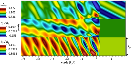
Figure 1: Ratios of the density and magnetic field components to their initial values for an incident entropy wave of amplitude $\delta\rho/\rho\approx 0.13$ and wavevector close to the resonance, interacting with the shock of setup 1, in a stationary regime. The transverse size of one panel is $\lambda_{y}\equiv 2\pi/k_{y}$.

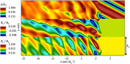
Figure 2: Snapshot from a simulation with the same parameters as in Fig. 1 but for an incident wave of larger amplitude $\delta\rho/\rho\approx 0.8$.

The typical timeline of a simulation is the following: as the incident wave impinges the shock front, corrugation develops and downstream modes are generated, then propagate away from the shock at their own group velocities. Close to the resonance, for small amplitude incoming waves, the amplitude of the corrugation increases slowly until it eventually reaches a stationary state, typically over a timescale of a few hundreds of $\omega^{-1}$. For non-resonant and/or large amplitude incoming waves, the final corrugation amplitude is reached on timescales of a few $\sim\omega^{-1}$, with some fluctuations though, for large amplitude incoming waves with a wavevector close to the resonance.

Once the source is shut off, the shock slowly regains planarity.

In the following, we first discuss the case of relativistic magnetized shock fronts, to make contact with the linear theory developed in LRG16, then we analyse the corrugation of sub-relativistic shock waves.

3.1 Interaction of an upstream mode with a relativistic shock front

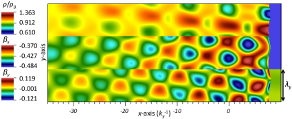
Figure 3: Downstream density and velocity profiles for an incoming magnetosonic wave of amplitude in density $\delta\rho/\rho\approx 0.45$ interacting with the shock of setup 2, at late times. $\rho_{0}=\rho_{2}$ is the initial downstream proper density and the color map was truncated to enhance the downstream structures.

We consider here the case of a relativistic shock wave (setups 1 and 2 of Table 1) for which $\Gamma_{1}\,\approx\,30$.

3.1.1 Incoming entropy modes – setup 1

Fig. 1 presents a snapshot of a simulation corresponding to setup 1, for an incoming entropy wave, i.e. density perturbations, with $\delta\rho/\rho\approx 0.13$ and a wavevector close to the resonance.

For small amplitude waves, corresponding to the linear interaction regime, the downstream medium can be described as a superposition of MHD modes, namely an entropy mode and two slow magnetosonic modes, plus a fast magnetosonic mode for wavevectors larger than the resonant one. As expected, we observed no downstream Alfvén waves since the specific geometry of these simulations is 2D. Indeed, setting the magnetic field in the plane of the simulation eliminates transverse waves (unless $k_{x}\,=\,0$, which would lead to degenerate Alfvén modes). This is not a strong restriction, since the linear theoretical analysis indicates that incoming compressible modes with a wavevector lying in the ($x$,$y$) plane are converted into outgoing compressible modes. To confirm this, we carried out dedicated 2.5D simulations, in which the spatial dependence of the physical fields is still 2D but where magnetic & velocity vectors can have arbitrary orientations in 3D. Such configuration hence allows transverse modes, but we did not find any trace of Alfvén waves. Therefore, these waves are likely to play a role only in full 3D configurations or for the case of incoming Alfvén waves. Incidentally, we also note that taking the background magnetic field along $z$ out of the simulation plane makes very little difference: the downstream turbulence structure appears somewhat simpler since for $\boldsymbol{k}\perp\boldsymbol{B}$, only fast magnetosonic modes can propagate.

Fig. 2 shows a snapshot from a simulation with the same physical parameters and numerical resolution as in Fig. 1, but for a larger amplitude of the incoming wave, $\delta\rho/\rho\approx 0.8$. The various flow quantities in the downstream medium are perturbed well into the non-linear regime, which leads to non-linear interactions remodelling the flow away from the shock and to the dissipation of small-scale structures.

3.1.2 Incoming fast magnetosonic modes – setup 2

We consider here a similar set-up as in the previous case, but for an incoming magnetosonic mode; in this case, all flow quantities of the upstream medium are perturbed, (see Appendix A). The simulations show qualitatively the same features as for entropy waves, with the same turbulence pattern at similar wavelengths. Fig. 3 shows an example in the non-linear regime, $\delta\rho/\rho\,\approx\,0.45$, away from the resonance (with $k_{x}$ smaller than the one giving rise to resonance). The initial perturbation is not visible as we expressed the density in units of the initial downstream density and the scale of the colormap was truncated to enhance the downstream structures. Here as well, we observe non-linear turbulence, with typical mildly relativistic velocities, on the downstream side, which is remodelled through non-linear interactions in time, i.e. away from the shock. The dissipation we observe is mainly of numerical nature but could also be partly accounted for by destructive interference and by the surface mode with complex $k_{x}$ mentioned in Sec. 2.3.

3.1.3 Transfer function

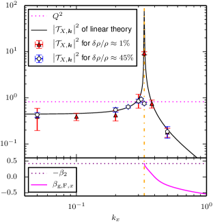
Figure 4: Top panel: squared modulus of the transfer function $\mathcal{T}_{X,\boldsymbol{k}}$ for an incoming entropy wave as a function of $k_{x}$, for setup 1 and $k_{y}=1$ in arbitrary units. The transverse size of the box is $2\pi$ in these units. The solid black curve plots the prediction of the linear analysis of LRG16; the symbols correspond to the results of our MHD simulations, in triangles for a small-amplitude wave $\delta\rho/\rho\,\approx\,0.01$ and in circles for a large-amplitude wave $\delta\rho/\rho\,\approx\,0.45$. The error bars give the measurement uncertainty on the corrugation amplitude $\Delta X_{\boldsymbol{k}}$ due to the finite resolution or to small non-stationarity for resonant large amplitude waves. The dotted line indicates the measure $Q^{2}$ of the perturbation of the upstream energy momentum tensor in units of $\delta\psi$. In the bottom panel, we plot the corresponding (analytically computed) group velocity along $x$ of the outgoing downstream fast magnetosonic mode; it intersects the shock speed line at the resonant $k_{x}$, which confirms the origin of the resonance seen in the upper panel. All quantities are evaluated in the downstream rest-frame.

The induced corrugation can be quantified through a transfer function,

$$\mathcal{T}_{X,\boldsymbol{k}}\,\equiv\,k_{y}\,\frac{\Delta X_{\boldsymbol{k}}}{\delta\psi},$$ (11)

which relates the amplitude $\delta\psi$ of the incoming wave displaying a wavevector $\boldsymbol{k}=(k_{x},k_{y})$ and, the corrugation amplitude $\Delta X_{\boldsymbol{k}}$ (see Appendix A for the definition of $\delta\psi$). The $k_{y}$ factor ensures that $\mathcal{T}_{X,\boldsymbol{k}}$ is a dimensionless quantity; if the transverse wavelength is increased, $\Delta X_{\boldsymbol{k}}$ will increase as much and $\mathcal{T}_{X,\boldsymbol{k}}$ will remain unchanged.

The corrugation amplitude, $\Delta X_{\boldsymbol{k}}$, is the amplitude along the $x$-direction of the rippled shock. In a fluid approach, the shock theoretically corresponds to a discontinuity appearing in some physical quantities. In our simulations however, its width is finite because of numerical diffusion, but is still much smaller than the corrugation scale, provided the resolution is high enough. We can then, quite arbitrarily, materialize the shock location as the line of cells where one of these fields (the density or the Lorentz factor, for instance) is the average of the background upstream and downstream values. The corrugation amplitude is then simply half of the peak-to-peak amplitude of the deformation of this line.

The definition of an amplitude $\delta\psi$ for the incoming wave is also somewhat arbitrary, because although the various flow variables all scale linearly with $\delta\psi$ (see Appendix A), they do so differently in terms of $k_{x}$ and $k_{y}$. This simultaneous dependence on $\delta\psi$ and $k_{x}$ notably implies that, at fixed $\delta\psi$, the perturbations of the components of the energy-momentum tensor evolve in non-trivial (and different) ways in terms of $k_{x}$. It is thus possible, in principle, to send in a wave with $\delta\psi\,\ll\,1$ which corresponds to a large perturbation of the energy or momentum flux along the shock normal, and which leads to a large response of the shock front. In order to distinguish such a response from a resonant response, we also keep track of the following quantity:

$$Q\,\equiv\,\frac{1}{\sqrt{2}\delta\psi}\left[\left(\frac{\delta T^{tx}}{T^{tx}}\right)^{2}+\left(\frac{\delta T^{xx}}{T^{xx}}\right)^{2}\right]^{1/2}$$ (12)

where $\delta T^{\mu\nu}$ and $T^{\mu\nu}$ are the perturbed and unperturbed energy-momentum tensors of the upstream plasma. $Q$ thus provides a measure of the perturbation in the incoming energy-momentum flux in units of $\delta\psi$ and the resonant response we are looking for is such that ${\mathcal{T}_{X,\boldsymbol{k}}}^{2}>Q^{2}$.

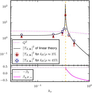
Figure 5: Same as Fig. 4 for an incoming fast magnetosonic mode corresponding to setup 2 with $k_{y}=1$ (arbitrary units) and wave amplitudes as indicated. All quantities are evaluated in the downstream rest-frame.

We compare here the transfer functions, obtained by solving numerically the shock crossing conditions perturbed at the first order as presented in LRG16 (black curve) and by measuring the shock deformation in the simulations (data points). Figure 4 corresponds to the entropy wave of Sect. 3.1 (setup 1) and Fig. 5 to the fast magnetosonic mode of Sect. 3.2 (setup 2). The error bars give the measurement uncertainty on the corrugation amplitude due to the finite resolution and to some non-stationary features close to the resonance for large amplitude waves. The dotted lines shown in the upper panels of these figures give the value of $Q^{2}$, for comparison to ${\mathcal{T}_{X,\boldsymbol{k}}}^{2}$ as discussed above. In Fig. 4, this dependence is trivial $Q\,\approx\,1$, since for entropy modes, the perturbations are independent of the wavevector, but in Fig. 5, $Q$ depends somewhat on $k_{x}$; such a dependence will be exacerbated in the sub-relativistic case of setup 3 that we study next.

Both figures clearly reveal a resonant response of the shock corrugation to the incoming perturbation, in good agreement with the prediction of the linear theory. In each figure, the lower panel plots the group velocity along $x$ of the outgoing fast magnetosonic mode as a function of the incoming longitudinal wavenumber. These panels confirm that the resonance occurs when the outgoing mode travels at a velocity close to that of the shock front. For values of $k_{x}$ smaller than the resonant one, the group velocity becomes complex, as the mode then turns into a surface wave located on the shock front, see the discussion above.

As an order of magnitude, for the small amplitude entropy wave simulations, for which $\delta\psi\,=\,\delta\rho/\rho$, $k\Delta X_{\boldsymbol{k}}\approx 3.8\delta\psi$ close to the resonance while $k\Delta X_{\boldsymbol{k}}\approx 0.5\delta\psi$ at large $k_{x}$. Linear theory predicts a more pronounced resonance with $k\Delta X_{\boldsymbol{k}}\,\gtrsim\,10\delta\psi$.

Figures 4 and 5 also plot the response of the shock to perturbations of significant amplitude, $\delta\rho/\rho\,\approx\,0.45$, beyond the reach of linear theory. We observe that the resonance remains, but that it is smoothed out with a typical response $k\Delta X_{\boldsymbol{k}}\,\approx\,1$, as anticipated in Lemoine (2016). The observed smoothing is rather evocative of a non-linear resonance broadening effect; it likely results from the non-linear couplings of the MHD equations, which become sizable at large amplitude, and which imply that the eigenmodes of linear MHD have a finite lifetime against conversion. This scaling $k\Delta X_{\boldsymbol{k}}\,\approx\,1$ is compared in Fig. 6 against the simulations of setup 1 at various wave amplitudes.

Figure 6: $k\Delta X_{\boldsymbol{k}}/\delta\psi$ measured in the simulations of setup 1 close to the resonance for incoming entropy waves of increasing amplitudes $\delta\psi=\delta\rho/\rho$.

3.2 Interaction with a sub-relativistic shock front

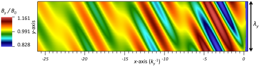
Figure 7: Downstream transverse magnetic field (in units of the initial downstream magnetic field $B_{0}=B_{2}$) of a simulation of setup 3, corresponding to the interaction of a fast magnetosonic mode with a sub-relativistic shock front, at small wave amplitude $\delta\rho/\rho=3\%$ with a wavevector close to the resonance, at late times. The color map was truncated to enhance the downstream structures.

The analytical study of LRG16 was conducted in the ultra-relativistic limit, to simplify the algebra, but there is no obvious physical reason why resonant corrugation should be a feature of relativistic shocks alone. In this section, we are thus interested in sub-relativistic shock velocities and present the results of simulations run for setup 3; whose parameters are close to what one can encounter in supernovae remnants (see Table 1).

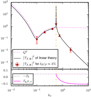
Figure 8: Transfer function and group velocity of the outgoing fast mode for an incoming fast wave of setup 3 for $k_{y}=1$. Notations similar to Figs. 4 and 5.

Fig. 7 presents a snapshot from such simulations and is rather similar to Fig. 1, 2 and 3, with the transmission of modes and their subsequent evolution downstream of the shock.

Fig. 8 presents the corresponding transfer function. As in Fig. 4 and 5, the solid curve indicates the predictions of linear theory, borrowed from LRG16 and adapted to the conditions of a sub-relativistic shock. The theory still predicts a resonant response when the outgoing fast magnetosonic mode surfs on the shock, as indicated by the lower panel. This resonance is clearly recovered in the MHD simulations, at least for small amplitude waves.

Note the dotted line in the upper panel: as before, it represents the quantity $Q^{2}$, which is related to the perturbation of the incoming energy-momentum in units of the perturbation amplitude $\delta\psi$. In the present case, however, this value depends strongly on the incoming wavenumber, in particular, $Q\,\gg\,1$ for $k_{x}\,\ll\,k_{y}$. This behaviour leads to a large perturbation of the incoming energy-momentum even though $\delta\rho/\rho\,\ll\,1$, hence to a large corrugation at small $k_{x}$. This peculiar $k_{x}$-dependence of the perturbation appears to be a feature of fast modes at a low beta-parameter of the plasma rather than a feature of the sub-relativistic regime.

4 Summary and discussion

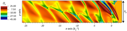
Figure 9: Non-vanishing component of the relativistic vorticity field $\Omega^{i}=\epsilon^{ij}_{\ \ k}\partial_{j}(w\Gamma\beta^{k}/\rho)$ in units of $c^{2}k_{y}$ for the same snapshot as in Fig. 2 (incoming entropy wave of amplitude $\delta\rho/\rho\approx 0.8$.)

In this paper, we have discussed 2D SRMHD simulations of a fast perpendicular shock corrugated by upstream sinusoidal entropy or magnetosonic waves, in both the relativistic and sub-relativistic flow velocity regimes. We have measured the transfer function which relates the amplitude of the corrugation $\Delta X_{k}$ to that of the incoming wave $\delta\psi$ and compared it to the predictions of the recent linear model described in LRG16. The main result of the present study is that we confirm the existence of a resonant response of the corrugation, in both the relativistic and the sub-relativistic regimes, when the fast magnetosonic mode that is produced downstream of the shock travels at a velocity comparable to that of the shock front. The interpretation of this resonance is as follows (see LRG16): as the incoming upstream mode interacts with the shock, it is transmitted into downstream MHD modes, including one fast magnetosonic mode which travels possibly as fast as the shock; if this resonance is satisfied, this mode surfs on and communicates its energy to the shock front, leading to a large – possibly formally infinite in the linear theory – response of the corrugation pattern. This resonance appears universal in the sense that, for any setup, for any incoming perturbation, at any perpendicular wavenumber, there exists at least one value of the longitudinal wavenumber which satisfies the resonance criterion.

It may be worth noting that the problem that we discuss here differs from the Richtmyer-Meshkov instability (RMI) (Richtmyer, 1960; Meshkov, 1969; Brouillette, 2002; Delmont et al., 2009; Nishihara et al., 2010). The standard RMI corresponds to the growth of the perturbation on an oblique or corrugated interface separating two fluids after it has encountered a planar shock wave, whereas we have studied the response of a flat shock front to its interaction with a compressive perturbation described by a plane wave. Some authors have recently extended the study of the RMI to the case in which the shock interacts with a continuous interface separating states of different densities with a given contrast $A=(\rho_{2}-\rho_{1})/(\rho_{2}+\rho_{1})$ over a finite length scale $\lambda$, see e.g. Brouillette & Sturtevant (1994). The problem that we have addressed then resembles somewhat this latter configuration, since the entropy mode induces a change in density, from $\rho_{1}=\rho-\delta\rho$ to $\rho_{2}=\rho+\delta\rho$ over a length scale $\pi/k_{x}$, although it repeats this inversion an indefinite amount of time, while in the above problem, there is only one interface. The previous authors observe that the growth rate of the RMI falls with increasing $\lambda$, and decreases with decreasing $A$ as the original RMI. Zou et al. (2017), on the other hand, examined the case of a rippled shock interacting with a flat interface and found growth rates much smaller than those of the "standard" RMI. Both studies however report hydrodynamic experiments only and the picture probably depends on the orientation and strength of the magnetic field in the MHD case; parallel shocks for example, prevent the deposition of vorticity at the interface (Sano et al., 2013, e.g.). In brief, the situation we simulated is quite different, we considered waves instead of a unique interface and even if triggered, it would seem that the growth rate of the instability is too small to be observed within the crossing time of the simulated downstream medium (see Fig. 9 for the relativistic vorticity field (Sironi & Goodman, 2007, e.g.) corresponding to the snapshot of Fig.2).

The resonance which we observe is more evocative of the “spontaneous emission of acoustic modes” described by D’Iakov (1958). This author considered the interaction of a mode originating from downstream and interacting with a purely hydrodynamic shock; he showed that this mode was reflected into the downstream medium with a reflection coefficient that could formally become infinite, whence the possibility of mode emission in the absence of a perturbation. This spontaneous emission has been discussed by a number of authors since then, see in particular Kontorovich (1958, 1959), Landau & Lifshitz (1987) for more qualitative explanations, see Bates & Montgomery (2000) and Stone & Edelman (1995) for numerical illustrations. In our framework, the incoming mode from upstream is transmitted through the shock into downstream outgoing modes; the amplitude of these modes, just as the amplitude of the shock corrugation, can be obtained through the inversion of the response matrix of the linear system. Zeros in the determinant of this system then lead to infinitely large responses, or spontaneous emission. We observe here that this spontaneous emission can (at least) take place for some specific values of the longitudinal wavenumber, when the outgoing mode surfs on the shock; to our knowledge, this had not been noticed before.

For simulations of large amplitude incident waves, the resonance is partly smoothed out due to some non-linear resonance broadening. At wave amplitudes outside the realm of linear theory, i.e. $\delta\psi\,\sim\,\mathcal{O}(1)$, we observe $k\delta X_{k}\,\approx\,1$, whereas $k\Delta X_{k}/\delta\psi>1$ at $\delta\psi\,\ll\,1$. One caveat is that we have modelled the large amplitude waves with linear eigenmodes, which are no longer true eigenmodes of the system of MHD equations; these waves thus tend to decay into other modes before they enter the shock. It would prove interesting to conduct simulations with exact non-linear (simple wave) solutions of the MHD equations.

In principle, the above resonant response of shock corrugation to incoming perturbations may find various astrophysical applications, since the resulting turbulence may have a number of phenomenological consequences, see e.g. the discussion in Sec. 1. As a next step in such direction, it would prove useful to conduct large-scale, high resolution simulations of the interaction of a shock front with a well developed spectrum of turbulence (as compared to the present case of a harmonic wave), making sure that the resolution in $k-$space is sufficient to probe the effect of the resonance. It would also be highly beneficial to conduct test-particle simulations, or even hybrid Particle-in-Cell/MHD simulations, in order to study how the corrugation pattern influences the acceleration process at shock waves, and how the accelerated particles themselves can induce corrugation through the instabilities that they develop in the shock precursor. Incidentally, we note that in a recent paper, van Marle et al. (2017) precisely observe the development of an unstable corrugated configuration, triggered by the interplay of the injection mechanism with the seeding of turbulence upstream of a corrugated shock.

Appendix A Linear SRMHD eigenmodes

In MHD, an infinite homogeneous system initially at stationary equilibrium can develop 7 linearly independent wave modes:

• one entropy wave (index _E): perturbation in the density field only;

• two Alfvén waves: incompressible and transverse modes;

• two slow magnetosonic modes;

• two fast magnetosonic modes (index _F).

For our purposes, the structure of the perturbations $\mathrm{\delta\xi}_{\boldsymbol{k}}\equiv(\delta\rho,\delta p_{\mathrm{th}},\delta\beta_{x},\delta\beta_{y},\delta B_{x},\delta B_{y})$ of entropy and fast magnetosonic modes in a plasma drifting at velocity $\beta_{0}=-\left(1-1/{\Gamma_{0}}^{2}\right)^{1/2}$ in the $x$-direction, initially characterized by the equilibrium $(\rho_{0},p_{\mathrm{th},0},\beta_{0},0,0,B_{0})$ read:

$$\mathrm{\delta\xi}_{\boldsymbol{k},\mathrm{E}}=\left(\rho_{0},0,0,0,0,0\right)\delta\psi_{\boldsymbol{k},\mathrm{E}},$$ (13)

$$\mathrm{\delta\xi}_{\boldsymbol{k},\mathrm{F}}=\left(\frac{{\omega^{\prime}_{F}}^{2}-{\beta_{\rm A}}^{2}{k^{\prime}}^{2}c^{2}}{{\beta_{\rm s}}^{2}\left(1-{\beta_{\rm A}}^{2}\right){k^{\prime}_{x}}^{2}c^{2}}\rho_{0},\frac{{\omega^{\prime}_{\rm F}}^{2}-{\beta_{\rm A}}^{2}{k^{\prime}}^{2}c^{2}}{{k^{\prime}_{x}c^{2}}^{2}}W_{0},\frac{\omega^{\prime}_{\rm F}}{{\Gamma_{0}}^{2}k^{\prime}_{x}c},\frac{{\beta_{\rm s}}^{2}\omega^{\prime}_{\rm F}k^{\prime}_{y}c}{\Gamma_{0}\left({\omega^{\prime}_{\rm F}}^{2}-{\beta_{\rm s}}^{2}{k^{\prime}_{y}}^{2}c^{2}\right)},-\frac{k^{\prime}_{y}}{k^{\prime}_{x}}\frac{B_{0}}{\Gamma_{0}},B_{0}\left(1+\beta_{0}\frac{\omega^{\prime}_{\rm F}}{{k^{\prime}_{x}c}}\right)\right)\delta\psi_{\boldsymbol{k},\mathrm{F}},$$ (14)

where $\delta\psi_{\boldsymbol{k},\mathrm{E/F}}\equiv\delta\psi\cos(\boldsymbol{k}\cdot\mathbf{x}-\omega_{\mathrm{E/F}}t)$ is the harmonic amplitude and primes denote proper quantities measured in the rest frame of the plasma. Naturally, the velocity/magnetic perturbations in the lab-frame are just the Lorentz-transformed plasma rest-frame perturbations. $\omega^{\prime}$ is linked to $\mathrm{k^{\prime}}$ through the dispersion relation

$$\omega^{\prime}_{E}=0,$$ (15)

$$\omega^{\prime}_{\rm F}=\pm\frac{c}{\sqrt{2}}\left\{{\beta_{\rm F}}^{2}{k^{\prime}}^{2}+{\beta_{\rm A}}^{2}{\beta_{\rm s}}^{2}{k^{\prime}_{y}}^{2}+\left[\left({\beta_{\rm F}}^{2}{k^{\prime}}^{2}+{\beta_{\rm A}}^{2}{\beta_{\rm s}}^{2}{k^{\prime}_{y}}^{2}\right)^{2}-4{\beta_{\rm A}}^{2}{\beta_{\rm s}}^{2}{k^{\prime}_{y}}^{2}{k^{\prime}}^{2}\right]^{1/2}\right\}^{1/2},$$ (16)

which involves the characteristic speeds, namely: the sound speed, ${\beta_{\rm s}}\,\equiv\,\left(\gamma_{\mathrm{eq}}p_{\mathrm{th},0}/w_{0}\right)^{1/2}$, the Alfvén speed, ${\beta_{\rm A}}\,=\,{B_{0}}/\left({4\pi\Gamma_{0}}^{2}W_{0}\right)^{1/2}$ and the fast speed, $\beta_{\rm F}=\left({\beta_{\rm A}}^{2}+{\beta_{\rm s}}^{2}-{\beta_{\rm A}}^{2}{\beta_{\rm s}}^{2}\right)^{1/2}$.

Appendix B Enforcing divergence-free magnetic field in SRMHD

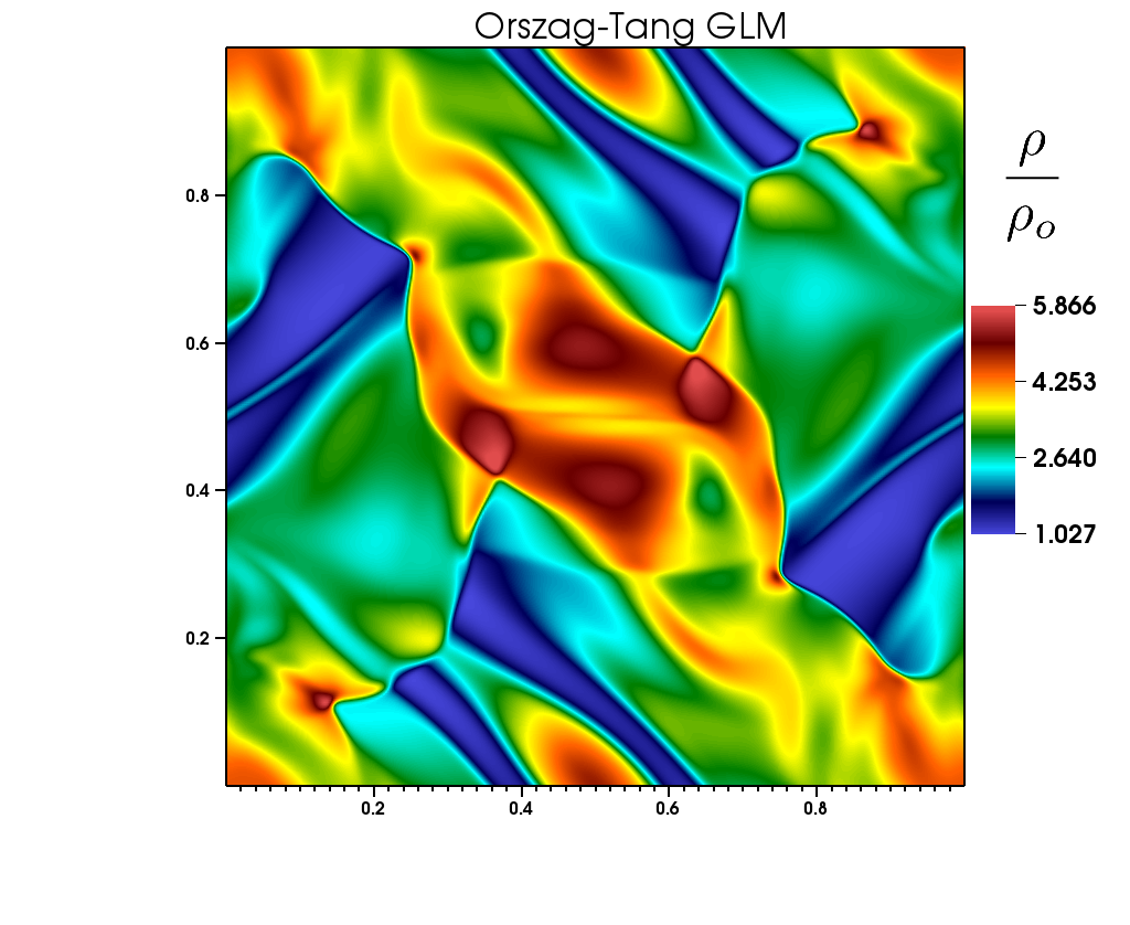
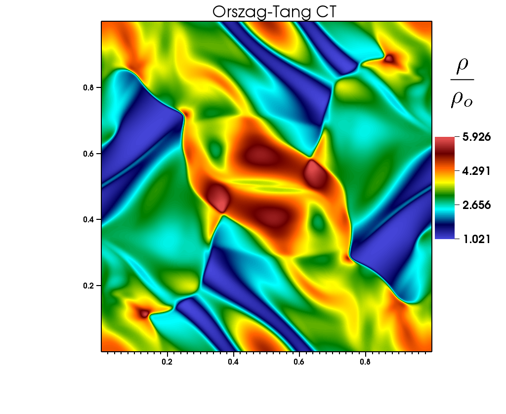
Figure 10: Simulations of the relativistic Orszag-Tang test performed with the MPI-AMRVAC code using the exact same numerical setup apart for the magnetic divergence cleaning method, namely the GLM (left) and the constrained transport (right). The proper density of the plasma is displayed at the same point in time, namely $t=1$. The overall density distributions are nearly identical except for some regions as the center of the computational domain or thin mass filaments appearing near the left and right boundaries. These regions actually correspond to areas of the computational domain where the divergence of the magnetic field remains high when using the standard GLM method (see Fig.11).

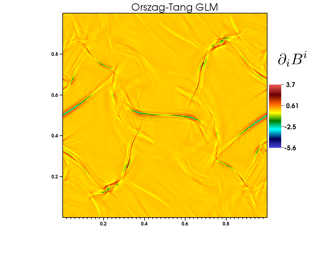
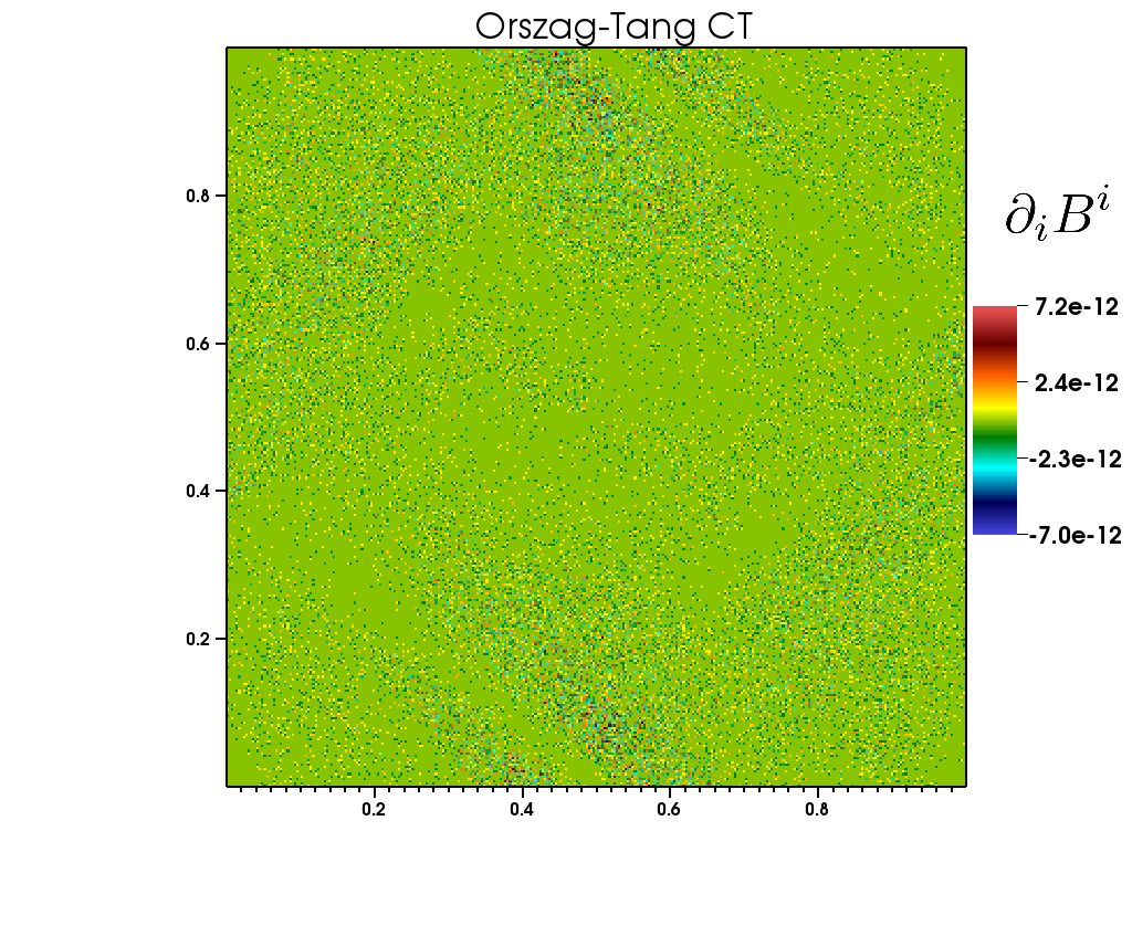
Figure 11: Colormaps of the divergence of the magnetic field for two simulations considering the relativistic Orszag-Tang problem with two different magnetic divergence cleaning approaches. The standard hyperbolic divergence cleaning (GLM) does maintain $\partial_{i}B^{i}$ to low level except in some narrow regions whereas constrained transport provides vanishing magnetic divergence to machine precision. The regions exhibiting large non-vanishing magnetic divergence actually correspond to areas where the two simulations exhibit small discrepancies regarding plasma quantities.

All the simulations presented in this paper were performed using a constrained transport (CT) scheme on top of the MHD solver, following the approach of Balsara & Spicer (1999). The MPI-AMRVAC code also hosts several schemes aiming at cleaning the divergence of the magnetic field. Among these schemes, one of the most efficient one is the hyperbolic divergence cleaning (GLM) developed by Dedner et al. (2002). We have decided to implement the constrained transport method inside the MPI-AMRVAC code since considering SRMHD waves requires to maintain the divergence of the magnetic field to zero at machine precision. Such statement is especially important when considering incoming waves onto a shock discontinuity.
In order to illustrate the impact of the magnetic divergence cleaning methods in SRMHD simulations, we present results of simulations dealing with the famous Orszag-Tang vortex test (Orszag & Tang, 1979). The relativistic version of this test has been presented in various studies (e.g. Beckwith & Stone (2011) and references therein). The initial conditions of the simulation are $\rho=25/9$, $P=5/3$ while velocity and magnetic field stand as

$$\beta_{x} = -\beta_{o}\sin(2\pi y)$$

$$\beta_{y} = \beta_{o}\sin(2\pi x)$$

$$B_{x} = -\sin(2\pi y)$$

$$B_{y} = \sin(4\pi x)$$

where $\beta_{o}=0.5$ is the maximal velocity of the fluid. The computational domain ranges from zero to unity in both $x$ and $y$ directions while having a grid resolution of $320\times 320$ cells. The simulation has been performed using a TVDLF solver coupled to a minmod slope limiter. Let us also mention that the all boundaries are periodic.

We have displayed in Fig.10 the proper density distribution of the plasma at identical time ($t=1$) for two simulations using different divergence cleaning methods, namely GLM and CT. The two distributions are globally very similar apart in some regions as for instance in the center of the computational domain. Indeed in this region, the GLM simulation has led to a smoother variation of the density compared to the one obtained using the CT algorithm. The same statement actually holds for the magnetic energy density. We can also mention that density filaments appearing in the left and right low density regions are thicker in the GLM simulation than in the CT one. Since both simulations use the very same setup apart from the divergence cleaning approaches, it is likely that these (small) discrepancies stems from local non-zero magnetic divergence. In Fig.11 we have displayed the colormaps of $\partial_{i}B^{i}$ for the two aforementioned simulations. We then clearly see that large non-vanishing magnetic divergence occurs in zones where the two simulations exhibit differences.

Relativistic simulations of astrophysical shocks deal with fluid velocities very close to the speed of light. Applying an efficient GLM approach to this kind of simulation may become difficult as the relaxation velocity of magnetic monopoles may not catch up with the fluid evolution, leading to unphysical errors. Among the various magnetic divergence cleaning algorithms published in the literature, we choose to employ the flux constrained transport approach as it provides an efficient way to get rid of magnetic monopoles while preventing any overestimation of the corrugation of the shock (see also the discussion in Tóth, 2000).

References

- Achterberg & Blandford (1986) Achterberg A., Blandford R. D., 1986, Month. Not. Roy. Astron. Soc., 218, 551
- Balsara & Spicer (1999) Balsara D. S., Spicer D. S., 1999, Journal of Computational Physics, 149, 270
- Balsara et al. (2001) Balsara D., Benjamin R. A., Cox D. P., 2001, ApJ, 563, 800
- Bates & Montgomery (2000) Bates J. W., Montgomery D. C., 2000, Physical Review Letters, 84, 1180
- Beckwith & Stone (2011) Beckwith K., Stone J. M., 2011, in American Astronomical Society Meeting Abstracts #218. p. 207.04
- Blandford & Eichler (1987) Blandford R., Eichler D., 1987, Phys. Rep., 154, 1
- Brouillette (2002) Brouillette M., 2002, Annual Review of Fluid Mechanics, 34, 445
- Brouillette & Sturtevant (1994) Brouillette M., Sturtevant B., 1994, Journal of Fluid Mechanics, 263, 271
- Bykov & Treumann (2011) Bykov A. M., Treumann R. A., 2011, A&ARv, 19, 42
- Bykov et al. (2008) Bykov A. M., Uvarov Y. A., Ellison D. C., 2008, ApJ, 689, L133
- Bykov et al. (2011) Bykov A. M., Ellison D. C., Osipov S. M., Pavlov G. G., Uvarov Y. A., 2011, ApJ, 735, L40
- D’Iakov (1958) D’Iakov S. P., 1958, Soviet Journal of Experimental and Theoretical Physics, 6, 739
- Dedner et al. (2002) Dedner A., Kemm F., Kröner D., Munz C.-D., Schnitzer T., Wesenberg M., 2002, Journal of Computational Physics, 175, 645
- Delmont et al. (2009) Delmont P., Keppens R., van der Holst B., 2009, Journal of Fluid Mechanics, 627, 33
- Drake & Gregori (2012) Drake R. P., Gregori G., 2012, ApJ, 749, 171
- Giacalone & Jokipii (2007) Giacalone J., Jokipii J. R., 2007, ApJ, 663, L41
- Goedbloed et al. (2010) Goedbloed J. P., Keppens R., Poedts S., 2010, Advanced magnetohydrodynamics with applications to laboratory and astrophysical plasmas. Cambridge University Press
- Guo & Giacalone (2010) Guo F., Giacalone J., 2010, ApJ, 715, 406
- Guo et al. (2012) Guo F., Li S., Li H., Giacalone J., Jokipii J. R., Li D., 2012, ApJ, 747, 98
- Inoue et al. (2011) Inoue T., Asano K., Ioka K., 2011, ApJ, 734, 77
- Johlander et al. (2016) Johlander A., et al., 2016, Physical Review Letters, 117, 165101
- Keppens et al. (2012) Keppens R., Meliani Z., van Marle A. J., Delmont P., Vlasis A., van der Holst B., 2012, Journal of Computational Physics, 231, 718
- Kontorovich (1958) Kontorovich V. M., 1958, Soviet Journal of Experimental and Theoretical Physics, 34, 127
- Kontorovich (1959) Kontorovich V. M., 1959, Soviet Journal of Experimental and Theoretical Physics, 34, 127
- Landau & Lifshitz (1987) Landau L. D., Lifshitz E. M., 1987, Fluid Mechanics (Second Edition): Course of Theoretical Physics, Volume 6. Pergamon Press
- Lemoine (2016) Lemoine M., 2016, Journal of Plasma Physics, 82, 635820401
- Lemoine et al. (2016) Lemoine M., Ramos O., Gremillet L., 2016, ApJ, 827, 44
- Lubchich & Despirak (2005) Lubchich A. A., Despirak I. V., 2005, Annales Geophysicae, 23, 1889
- Lyutikov et al. (2012) Lyutikov M., Balsara D., Matthews C., 2012, Month. Not. Roy. Astron. Soc., 422, 3118
- Marcowith et al. (2016) Marcowith A., et al., 2016, Reports on Progress in Physics, 79, 046901
- Mathews (1971) Mathews W., 1971, ApJ, 165, 147
- McKenzie & Westphal (1970) McKenzie J. F., Westphal K. O., 1970, Physics of Fluids, 13, 630
- Meliani et al. (2004) Meliani Z., Sauty C., Tsinganos K., Vlahakis N., 2004, A&A, 425, 773
- Meshkov (1969) Meshkov E. E., 1969, Fluid Dynamics, 4, 101
- Mignone & McKinney (2007) Mignone A., McKinney J. C., 2007, MNRAS, 378, 1118
- Moiseev & Sagdeev (1963) Moiseev S. S., Sagdeev R. Z., 1963, Journal of Nuclear Energy, 5, 43
- Moullard et al. (2006) Moullard O., Burgess D., Horbury T. S., Lucek E. A., 2006, Journal of Geophysical Research (Space Physics), 111, A09113
- Nishihara et al. (2010) Nishihara K., Wouchuk J. G., Matsuoka C., Ishizaki R., Zhakhovsky V. V., 2010, Phil. Trans. R. Soc. A, 368, 1769
- Orszag & Tang (1979) Orszag S. A., Tang C.-M., 1979, Journal of Fluid Mechanics, 90, 129
- Richtmyer (1960) Richtmyer R. D., 1960, Commun. Pure Appl. Math., XIII, 297
- Sano et al. (2013) Sano T., Inoue T., Nishihara K., 2013, Phys. Rev. Lett., 111, 205001
- Schaeffer et al. (2017) Schaeffer D. B., Fox W., Haberberger D., Fiksel G., Bhattacharjee A., Barnak D. H., Hu S. X., Germaschewski K., 2017, Physical Review Letters, 119, 025001
- Sironi & Goodman (2007) Sironi L., Goodman J., 2007, Astrophys. J., 671, 1858
- Stone & Edelman (1995) Stone J. M., Edelman M., 1995, ApJ, 454, 182
- Synge (1957) Synge J., 1957, The relativistic gas. North-Holland Pub. Co.
- Taub (1948) Taub A. H., 1948, Physical Review, 74, 328
- Tóth (2000) Tóth G., 2000, Journal of Computational Physics, 161, 605
- Zankovich & Kovalenko (2015) Zankovich A. M., Kovalenko I. G., 2015, ApJ, 800, 28
- Zou et al. (2017) Zou L., Liu J., Liao S., Zheng X., Zhai Z., Luo X., 2017, Phys. Rev. E, 95, 013107
- Zrake (2016) Zrake J., 2016, ApJ, 823, 39
- van Marle et al. (2017) van Marle A. J., Casse F., Marcowith A., 2017, MNRAS, (in press),
- van der Holst et al. (2008) van der Holst B., Keppens R., Meliani Z., 2008, Computer Physics Communications, 179, 617