Accelerating GMM-based patch priors for image restoration: Three ingredients for a 100$\boldsymbol{\times}$ speed-up

Abstract

Image restoration methods aim to recover the underlying clean image from corrupted observations. The Expected Patch Log-likelihood (EPLL) algorithm is a powerful image restoration method that uses a Gaussian mixture model (GMM) prior on the patches of natural images. Although it is very effective for restoring images, its high runtime complexity makes EPLL ill-suited for most practical applications. In this paper, we propose three approximations to the original EPLL algorithm. The resulting algorithm, which we call the fast-EPLL (FEPLL), attains a dramatic speed-up of two orders of magnitude over EPLL while incurring a negligible drop in the restored image quality (less than 0.5 dB). We demonstrate the efficacy and versatility of our algorithm on a number of inverse problems such as denoising, deblurring, super-resolution, inpainting and devignetting. To the best of our knowledge, FEPLL is the first algorithm that can competitively restore a $512\!\times\!512$ pixel image in under 0.5s for all the degradations mentioned above without specialized code optimizations such as CPU parallelization or GPU implementation.

I Introduction

Patch-based methods form a very popular and successful class of image restoration techniques. These methods process an image on a patch-by-patch basis where a patch is a small sub-image (e.g., of $8\!\times\!8$ pixels) that captures both geometric and textural information. Patch-based algorithms have been at the core of many state-of-the-art results obtained on various image restoration problems such as denoising, deblurring, super-resolution, defogging, or compression artifact removal to name a few. In image denoising, patch-based processing became popular after the success of the Non-Local Means algorithm [2]. Subsequently, continued research efforts have led to significant algorithmic advancements in this area [1, 8, 39, 11, 27, 37, 24]. Other inverse problems such as image super-resolution and image deblurring have also benefited from patch-based models [9, 16, 30, 34, 14, 25].

Among these various patch-based methods, the Expected Patch Log-Likelihood algorithm (EPLL) [39] deserves a special mention due to its restoration performance and versatility. The EPLL introduced an innovative application of Gaussian Mixture Models (GMMs) to capture the prior distribution of patches in natural images. Note that a similar idea was introduced concurrently in [37]. The success of this method is evident from the large number of recent works that extend the original EPLL formulation [35, 26, 4, 29, 31, 18]. However, a persistent problem of EPLL-based algorithms is their high runtime complexity. For instance, it is orders of magnitude slower than the well-engineered BM3D image denoising algorithm [8]. However, extensions of BM3D that perform super-resolution [10] and other inverse problems [20] require fundamental algorithmic changes, making BM3D far less adaptable than EPLL. Other approaches that are as versatile as EPLL [33, 5, 19] either lack the algorithmic efficiency of BM3D or the restoration efficacy of EPLL.

Another class of techniques that arguably offers better runtime performance than EPLL-based methods (but not BM3D) are those based on deep learning. With the advancements in computational resources, researchers have attempted to solve some classical inverse problems using multi-layer perceptrons [3] and deep networks [6, 13, 21]. These methods achieve very good restoration performance, but are heavily dependent on the amount of training data available for each degradation scenario. Most of these methods learn filters that are suited to restore a specific noise level (denoising), blur (deblurring) or upsampling factor (super-resolution), which makes them less attractive to serve as generic image restoration solutions. More recently, Zhang et al. [38] demonstrated the use of deep residual networks for general denoising problems, single-image super-resolution and compression artifact removal. Unlike earlier deep learning efforts, their approach can restore images with different noise levels using a single model which is learned by training on image patches containing a range of degradations. Even in this case, the underlying deep learning model requires retraining whenever a new degradation scenario different from those considered during the learning stage is encountered. Moreover, it is much harder to gain insight into the actual model learned by a deep architecture compared to a GMM. For this reason, even with the advent of deep learning methods, flexible algorithms like EPLL that have a transparent formulation remain relevant for image restoration.

Recently, researchers have tried to improve the speed of EPLL by replacing the most time-consuming operation in the EPLL algorithm with a machine learning-based technique of their choice [36, 32]. These methods were successful in accelerating EPLL to an extent but did not consider tackling all of its bottlenecks. In contrast, this paper focuses on accelerating EPLL by proposing algorithmic approximations to all the prospective bottlenecks present in the original algorithm proposed by Zoran et al. [39]. To this end, we first provide a complete computational and runtime analysis of EPLL, present a new and efficient implementation of original EPLL algorithm and then finally propose innovative approximations that lead to a novel algorithm that is more than 100$\times$ faster compared to the efficiently implemented EPLL (and 350$\times$ faster than the runtime obtained by using the original implementation [39]).

Contributions

The main contributions of this work are the following. We introduce three strategies to accelerate patch-based image restoration algorithms that use a GMM prior. We show that, when used jointly, they lead to a speed-up of the EPLL algorithm by two orders of magnitude. Compared to the popular BM3D algorithm, which represents the current state-of-the-art in terms of speed among CPU-based implementations, the proposed algorithm is almost an order of magnitude faster. The three strategies introduced in this work are general enough to be applied individually or in any combination to accelerate other related algorithms. For example, the random subsampling strategy is a general technique that could be reused in any algorithm that considers overlapping patches to process images; the flat tail spectrum approximation can accelerate any method that needs Gaussian log-likelihood or multiple Mahalanobis metric calculations; finally, the binary search tree for Gaussian matching can be included in any algorithm based on a GMM prior model and can be easily adapted for vector quantization techniques that use a dictionary.

For reproducibility purposes, we release our software on GitHub along with a few usage demonstrations (available at https://goo.gl/xjqKUA).

II Expected Patch Log-Likelihood (EPLL)

We consider the problem of estimating an image ${\boldsymbol{x}}\in\mathbb{R}^{N}$ ($N$ is the number of pixels) from noisy linear observations ${\boldsymbol{y}}=\mathcal{A}{\boldsymbol{x}}+{\boldsymbol{w}}$, where $\mathcal{A}:\mathbb{R}^{N}\to\mathbb{R}^{M}$ is a linear operator and ${\boldsymbol{w}}\in\mathbb{R}^{M}$ is a noise component assumed to be white and Gaussian with variance $\sigma^{2}$. In a standard denoising problem $\mathcal{A}$ is the identity matrix, but in more general settings, it can account for loss of information or blurring. Typical examples for operator $\mathcal{A}$ are: a low pass filter (for deconvolution), a masking operator (for inpainting), or a projection on a random subspace (for compressive sensing). To reduce noise and stabilize the inversion of $\mathcal{A}$, some prior information is used for the estimation of ${\boldsymbol{x}}$. The EPLL introduced by Zoran and Weiss [39] includes this prior information as a model for the distribution of patches found in natural images. Specifically, the EPLL defines the restored image as the maximum a posteriori estimate, corresponding to the following minimization problem:

$$\underset{{\boldsymbol{x}}}{\operatorname{argmin}}\;\frac{P}{2\sigma^{2}}|\!|\mathcal{A}{\boldsymbol{x}}-{\boldsymbol{y}}|\!|^{2}-\sum_{i\in\mathcal{I}}\log p\left(\mathcal{P}_{i}{\boldsymbol{x}}\right)$$ (1)

where $\mathcal{I}=\{1,\ldots,N\}$ is the set of pixel indices, $\mathcal{P}_{i}:\mathbb{R}^{N}\to\mathbb{R}^{P}$ is the linear operator extracting a patch with $P$ pixels centered at the pixel with location $i$ (typically, $P=8\!\times\!8$), and $p(.)$ is the a priori probability density function (i.e., the statistical model of noiseless patches in natural images). While the first term in eq. (1) ensures that $\mathcal{A}{\boldsymbol{x}}$ is close to the observations ${\boldsymbol{y}}$ (this term is the negative log-likelihood under the white Gaussian noise assumption), the second term regularizes the solution ${\boldsymbol{x}}$ by favoring an image such that all its patches fit the prior model of patches in natural images. The authors of [39] showed that this prior can be well approximated (upon removal of the DC component of each patch) using a zero-mean Gaussian Mixture Model (GMM) with $K\!=\!200$ components, that reads for any patch ${\boldsymbol{z}}\in\mathbb{R}^{P}$, as

$$p\left({\boldsymbol{z}}\right)=\sum_{k=1}^{K}w_{k}\frac{1}{(2\pi)^{P/2}|{\boldsymbol{\Sigma}}_{k}|^{1/2}}\exp\left(-\frac{1}{2}{\boldsymbol{z}}^{t}{\boldsymbol{\Sigma}}_{k}^{-1}{\boldsymbol{z}}\right),$$ (2)

where the weights $w_{k}$ (such that $w_{k}\!>\!0$ and $\sum_{k}w_{k}\!=\!1$) and the covariance matrices ${\boldsymbol{\Sigma}}_{k}\in\mathbb{R}^{P\times P}$ are estimated using the Expectation-Maximization algorithm [12] on a dataset consisting of 2 million “clean” patches extracted from the training set of the Berkeley Segmentation (BSDS) dataset [28].

TABLE I: Comparison of the execution time of our implementation of EPLL with and without proposed accelerations. Experiment conducted on a $481\times 321$ image denoising problem. Profiling was carried out using MATLAB (R2014b) on a PC with Intel(R) Core(TM) i7-4790K CPU @4.00GHz and 16 GB RAM. Execution times are reported in seconds (s) and as a percentage of the total time (%).

Step	Without accelerations		With the proposed accelerations
(Gaussian selection)	NaNs	NaN %	NaNs	NaN %
(Patch estimation)	NaNs	NaN %	NaNs	NaN %
(Patch extraction)	NaNs	NaN %	NaNs	NaN %
(Patch reprojection)	NaNs	NaN %	NaNs	NaN %
Others	NaNs	NaN %	NaNs	NaN %
Total	45.69s		0.35s

Half-quadratic splitting

Problem (1) is a large non-convex problem where $\mathcal{A}$ couples all unknown pixel values ${\boldsymbol{x}}$ and the patch prior is highly non-convex. A classical workaround, known as half-quadratic splitting [15, 23], is to introduce $N$ auxiliary unknown vectors ${\boldsymbol{z}}_{i}\in\mathbb{R}^{P}$, and consider instead the penalized optimization problem that reads, for $\beta>0$, as

$$\underset{{\boldsymbol{x}},{\boldsymbol{z}}_{1},\ldots,{\boldsymbol{z}}_{N}}{\operatorname{argmin}}\;\frac{P}{2\sigma^{2}}|\!|\mathcal{A}{\boldsymbol{x}}-{\boldsymbol{y}}|\!|^{2}\\ +\frac{\beta}{2}\sum_{i\in\mathcal{I}}|\!|\mathcal{P}_{i}{\boldsymbol{x}}-{\boldsymbol{z}}_{i}|\!|^{2}-\sum_{i\in\mathcal{I}}\log p\left({\boldsymbol{z}}_{i}\right).$$ (3)

When $\beta\to\infty$, the problem (3) becomes equivalent to the original problem (1). In practice, an increasing sequence of $\beta$ is considered, and an alternating optimization scheme is used:

$$\biggl{\{}\hat{\boldsymbol{z}}_{i} \leftarrow\underset{{\boldsymbol{z}}_{i}}{\operatorname{argmin}}\;\frac{\beta}{2}|\!|\mathcal{P}_{i}\hat{\boldsymbol{x}}-{\boldsymbol{z}}_{i}|\!|^{2}-\log p\left({\boldsymbol{z}}_{i}\right)\biggr{\}}_{i=1..N}$$ (4)

$$\hat{\boldsymbol{x}} \leftarrow\underset{{\boldsymbol{x}}}{\operatorname{argmin}}\;\frac{P}{2\sigma^{2}}|\!|\mathcal{A}{\boldsymbol{x}}-{\boldsymbol{y}}|\!|^{2}+\frac{\beta}{2}\sum_{i\in\mathcal{I}}|\!|\mathcal{P}_{i}{\boldsymbol{x}}-\hat{\boldsymbol{z}}_{i}|\!|^{2}.$$ (5)

$$\text{for all }i\in\mathcal{I}$$

$$\makebox(0.0,0.0)[]{\hskip 13.56244pt\rule[-123.99951pt]{0.56905pt}{69.74973pt}}\quad\quad\tilde{\boldsymbol{z}}_{i}\leftarrow\mathcal{P}_{i}\hat{\boldsymbol{x}}$$ (Patch extraction)

$$\quad\quad k_{i}^{\star}\leftarrow\underset{1\leqslant k_{i}\leqslant K}{\operatorname{argmin}}\;\log w_{k_{i}}^{-2}+\log\left|{\boldsymbol{\Sigma}}_{k_{i}}\!+\!\tfrac{1}{\beta}\mathrm{Id}_{P}\right|+$$

$$\quad\quad\quad\quad\quad\quad\quad\quad\quad\tilde{\boldsymbol{z}}_{i}^{t}\left({\boldsymbol{\Sigma}}_{k_{i}}\!+\!\tfrac{1}{\beta}\mathrm{Id}_{P}\right)^{-1}\!\!\tilde{\boldsymbol{z}}_{i}$$ (Gaussian selection)

$$\quad\quad\hat{{\boldsymbol{z}}}_{i}\leftarrow\left({\boldsymbol{\Sigma}}_{k_{i}^{\star}}+\tfrac{1}{\beta}\mathrm{Id}_{P}\right)^{-1}{\boldsymbol{\Sigma}}_{k_{i}^{\star}}\tilde{\boldsymbol{z}}_{i}$$ (Patch estimation)

$$\tilde{\boldsymbol{x}}\leftarrow\big{(}\text{\small${\sum_{i\in\mathcal{I}}}$}\mathcal{P}_{i}^{t}\mathcal{P}_{i}\big{)}^{-1}\text{\small${\sum_{i\in\mathcal{I}}}$}\mathcal{P}_{i}^{t}\hat{\boldsymbol{z}}_{i}$$ (Patch reprojection)

$$\hat{\boldsymbol{x}}\leftarrow\big{(}\mathcal{A}^{t}\mathcal{A}+\beta\sigma^{2}\mathrm{Id}_{N}\big{)}^{-1}\left(\mathcal{A}^{t}{\boldsymbol{y}}+\beta\sigma^{2}\tilde{\boldsymbol{x}}\right)$$ (Image estimation)

Algorithm 1 The five steps of an EPLL iteration [39]

Algorithm

Subproblem (5) corresponds to solving a linear inverse problem with a Tikhonov regularization, and has an explicit solution often referred to as Wiener filtering:

$$\hat{{\boldsymbol{x}}}=\left(\mathcal{A}^{t}\mathcal{A}+\frac{\beta\sigma^{2}}{P}\sum_{i\in\mathcal{I}}\mathcal{P}_{i}^{t}\mathcal{P}_{i}\right)^{-1}\left(\mathcal{A}^{t}{\boldsymbol{y}}+\frac{\beta\sigma^{2}}{P}\sum_{i\in\mathcal{I}}\mathcal{P}_{i}^{t}\hat{\boldsymbol{z}}_{i}\right),$$ (6)

where $\mathcal{P}_{i}^{t}\mathcal{P}_{i}$ is a diagonal matrix whose $i$-th diagonal element corresponds to the number of patches overlapping the pixel of index $i$. This number is a constant equal to $P$ (assuming proper boundary conditions are used), which allows to split the computation into two steps Patch reprojection and Image estimation as shown in Alg. 1. Note that the step Patch reprojection is simply the average of all overlapping patches. In contrast, subproblem (4) cannot be obtained in closed form as it involves a term with the logarithm of a sum of exponentials. A practical solution proposed in [39] is to keep only the component $k_{i}^{\star}$ maximizing the likelihood for the given patch assuming it is a zero-mean Gaussian random vector with covariance matrix ${\boldsymbol{\Sigma}}_{k_{i}}+\tfrac{1}{\beta}\mathrm{Id}_{P}$. With this approximation, the solution of (4) is also given by Wiener filtering, and the resulting algorithm iterates the steps described in Alg. 1. The authors of [39] found that using $T\!=\!5$ iterations, with the sequence $\beta=\frac{1}{\sigma^{2}}\{1,4,8,16,32\}$, for the initialization $\hat{\boldsymbol{x}}={\boldsymbol{y}}$, provides relevant solutions in denoising contexts for a wide range of noise level values $\sigma^{2}$.

II-A Complexity via eigenspace implementation

The algorithm summarized in the previous section may reveal cumbersome computations as it requires performing numerous matrix multiplications and inversions. Nevertheless, as the matrices ${\boldsymbol{\Sigma}}_{k}$ are known prior to any calculation, their eigendecomposition can be computed offline to improve the runtime. If we denote the eigendecomposition (obtained offline) of ${\boldsymbol{\Sigma}}_{k}={\boldsymbol{U}}_{k}{\boldsymbol{S}}_{k}{\boldsymbol{U}}_{k}^{t}$, such that ${\boldsymbol{U}}_{k}\in\mathbb{R}^{P\times P}$ is unitary and ${\boldsymbol{S}}_{k}$ is diagonal with positive diagonal elements ordered in decreasing order, steps Gaussian selection and Patch estimation can be expressed in the space of coefficients ${\boldsymbol{c}}$ as

$$\biggl{\{}\tilde{\boldsymbol{c}}^{k}_{i}\leftarrow{\boldsymbol{U}}_{k}^{t}\tilde{\boldsymbol{z}}_{i}\biggr{\}}_{\begin{subarray}{c}\\[-7.00002pt] k=1..K\\ i=1..N\end{subarray}} \mathcal{O}(NKP^{2})$$ (7)

$$\biggl{\{}k_{i}^{\star}\leftarrow\underset{1\leqslant k\leqslant K}{\operatorname{argmin}}\;\iota^{k}+\sum_{j=1}^{P}\biggl{(}\log\nu^{k}_{j}+\frac{[\tilde{\boldsymbol{c}}^{k}_{i}]_{j}^{2}}{\nu^{k}_{j}}\biggr{)}\biggr{\}}_{i=1..N}$$

$$\mathcal{O}(NKP)$$ (8)

$$\biggl{\{}[\hat{{\boldsymbol{c}}}_{i}]_{j}\leftarrow\gamma^{k_{i}^{\star}}_{j}[\tilde{\boldsymbol{c}}^{k_{i}^{\star}}_{i}]_{j}\biggr{\}}_{\begin{subarray}{c}\\[-7.00002pt] j=1..P\\ i=1..N\end{subarray}} \mathcal{O}(NP)$$ (9)

$$\biggl{\{}\hat{\boldsymbol{z}}_{i}\leftarrow{\boldsymbol{U}}_{k_{i}^{\star}}\hat{{\boldsymbol{c}}}_{i}\biggr{\}}_{i=1..N} \mathcal{O}(NP^{2})$$ (10)

where $[\tilde{{\boldsymbol{c}}}]_{j}$ denotes the $j$-th entry of vector $\tilde{\boldsymbol{c}}$, $\iota^{k}=-2\log w_{k}$, $\nu^{k}_{j}=[{\boldsymbol{S}}_{k}]_{jj}\!+\!\tfrac{1}{\beta}$, and $\gamma^{k}_{j}=[{\boldsymbol{S}}_{k}]_{jj}/\nu^{k}_{j}$ with $[{\boldsymbol{S}}_{k}]_{jj}$ the $j$-th entry on the diagonal of matrix ${\boldsymbol{S}}_{k}$. The complexity of each operation is indicated on its right and corresponds to the number of operations per iteration of the alternate optimization scheme. The steps Patch extraction and Patch reprojection share a complexity of $\mathcal{O}(NP)$. Finally, the complexity of step Image estimation depends on the transform $\mathcal{A}$. In many scenarios of interest, $\mathcal{A}^{t}\mathcal{A}$ can be diagonalized using a fast transform and the inversion of $\mathcal{A}^{t}\mathcal{A}+\beta\sigma^{2}\mathrm{Id}_{N}$ can be performed efficiently in the transformed domain (since $\mathrm{Id}_{N}$ is diagonal in any orthonormal basis). For instance, it leads to $\mathcal{O}(N)$ operations for denoising or inpainting, and $\mathcal{O}(N\log N)$ for periodical deconvolutions or super-resolution problems, thanks to the fast Fourier transform. If $\mathcal{A}$ cannot be easily diagonalized, this step can be performed using conjugate gradient (CG) method, as done in [39], at a computational cost that depends on the number of CG iterations (i.e., on the conditioning of $\mathcal{A}^{t}\mathcal{A}+\beta\sigma^{2}\mathrm{Id}_{N}$). In any case, as shown in the next section, this step has a complexity independent of $P$ and $K$ and is one of the faster operations in the image restoration problems considered in this paper.

II-B Computation time analysis

In order to uncover the practical computational bottlenecks of EPLL, we have performed the following computational analysis. To identify clearly which part is time consuming, it is important to make the algorithm implementation as optimal as possible. Therefore, we refrain from using the MATLAB code provided by the original authors [39] for speed comparisons. Instead, we use a MATLAB/C version of EPLL based on the eigenspace implementation described above, where some steps are written in C language and interfaced using mex functions. This version, which we refer to as EPLLc, provides results identical to the original implementation while being 2-3 times faster. The execution time of each step for a single run of EPLLc is reported in the second column of Table I. Reported times fit our complexity analysis and clearly indicate that the Step Gaussian selection causes significant bottleneck due to $\mathcal{O}(NP^{2}K)$ complexity.

In the next section, we propose three independent modifications leading to an algorithm with a complexity of $\mathcal{O}(NP\bar{r}\log K/s^{2})$ with two constants $1\leqslant s^{2}\leqslant P$ and $1\leqslant\bar{r}\leqslant P$ that control the accuracy of the approximations introduced. The algorithm, in practice, is more than $100$ times faster as shown by its runtimes reported in the third column.

III Fast EPLL: the three key ingredients

We propose three accelerations based on (i) scanning only a (random) subset of the $N$ patches, (ii) reducing the number of mixture components matched, and (iii) projecting on a smaller subspace of the covariance eigenspace. We begin by describing this latter acceleration strategy in the following paragraph.

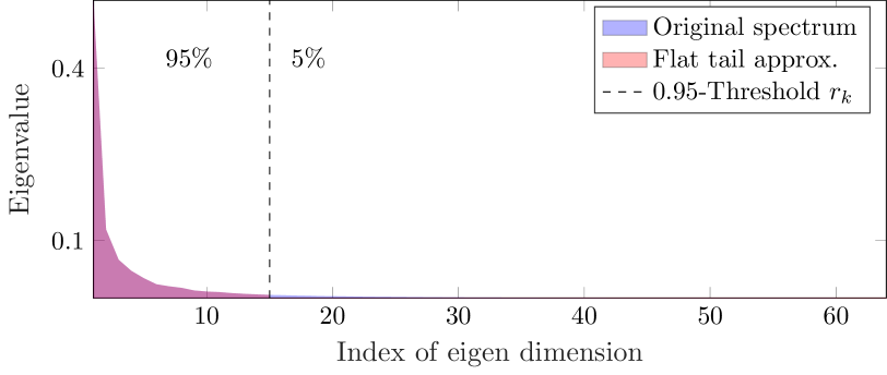
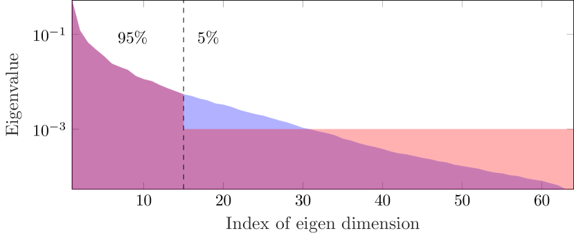
Figure 1: Flat tail approximation: (a) with eigenvalues display on linear and (b) logarithmic scale. The $r_{k}=15$ first eigen components explains $\rho\!=\!95\%$ of the variability.

III-A Speed-up via flat tail spectrum approximation

To avoid computing the $P$ coefficients of the vector $\tilde{c}_{i}^{k}$ in eq. (7), we rely on a flat-tail approximation. The $k$-th Gaussian model is said to have a flat tail if there exists a rank $r_{k}$ such that for any $j\!>\!r_{k}$, the eigenvalues are constant: $[{\boldsymbol{S}}_{k}]_{j,j}\!=\!\lambda_{k}$. Denoting by $\bar{\boldsymbol{U}}_{k}\!\in\!\mathbb{R}^{P\times r_{k}}$ (resp. $\bar{\boldsymbol{U}}_{k}^{c}\!\in\!\mathbb{R}^{P\times r_{k}^{c}}$) the matrix formed by the $r_{k}$ first (resp. $r_{k}^{c}\!=\!P\!-\!r_{k}$ last) columns of ${\boldsymbol{U}}_{k}$, we have $\bar{\boldsymbol{U}}_{k}^{c}(\bar{\boldsymbol{U}}_{k}^{c})^{t}\!=\!\mathrm{Id}_{P}\!-\!\bar{\boldsymbol{U}}_{k}\bar{\boldsymbol{U}}_{k}^{t}$. It follows

$$({\boldsymbol{\Sigma}}_{k}+\tfrac{1}{\beta}\mathrm{Id}_{P})^{-1} =\bar{\boldsymbol{U}}_{k}(\bar{\boldsymbol{S}}_{k}+\tfrac{1}{\beta}\mathrm{Id}_{r_{k}})^{-1}\bar{\boldsymbol{U}}_{k}^{t}$$

$$+(\lambda_{k}+\tfrac{1}{\beta})^{-1}(\mathrm{Id}_{P}-\bar{\boldsymbol{U}}_{k}\bar{\boldsymbol{U}}_{k}^{t}),$$ (11)

$$({\boldsymbol{\Sigma}}_{k}+\tfrac{1}{\beta}\mathrm{Id}_{P})^{-1}{\boldsymbol{\Sigma}}_{k} =\bar{\boldsymbol{U}}_{k}(\bar{\boldsymbol{S}}_{k}+\tfrac{1}{\beta}\mathrm{Id}_{r_{k}})^{-1}\bar{\boldsymbol{S}}_{k}\bar{\boldsymbol{U}}_{k}^{t}$$

$$+\lambda_{k}(\lambda_{k}+\tfrac{1}{\beta})^{-1}(\mathrm{Id}_{P}-\bar{\boldsymbol{U}}_{k}\bar{\boldsymbol{U}}_{k}^{t}),$$ (12)

where $\bar{\boldsymbol{S}}_{k}\in\mathbb{R}^{r_{k}\times r_{k}}$ is the diagonal matrix formed by the $r_{k}$ first rows and columns of ${\boldsymbol{S}}_{k}$. Steps Gaussian selection and Patch estimation can thus be rewritten as

$$\biggl{\{}\tilde{\boldsymbol{c}}^{k}_{i}\leftarrow\bar{\boldsymbol{U}}_{k}^{t}\tilde{\boldsymbol{z}}_{i}\biggr{\}}_{\begin{subarray}{c}\\[-7.00002pt] k=1..K\\ i=1..N\end{subarray}} \!\!\!\!\!\mathcal{O}(NKP\bar{r})$$ (13)

$$\biggl{\{}k_{i}^{\star}\leftarrow\underset{1\leqslant k\leqslant K}{\operatorname{argmin}}\;\iota_{k}+r_{k}^{c}\log\nu^{k}_{P}\!+\!\frac{|\!|\tilde{\boldsymbol{z}}_{i}|\!|^{2}}{\nu^{k}_{P}}$$

$$\hskip 8.5359pt\!+\!\sum_{j=1}^{r_{k}}\biggl{(}\log\nu^{k}_{j}\!+\!\frac{[\tilde{\boldsymbol{c}}^{k}_{i}]_{j}^{2}}{\nu^{k}_{j}}\!-\!\frac{[\tilde{\boldsymbol{c}}^{k}_{i}]_{j}^{2}}{\nu^{k}_{P}}\biggr{)}\biggr{\}}_{i=1..N} \mathcal{O}(NK\bar{r})$$ (14)

$$\biggl{\{}[\hat{{\boldsymbol{c}}}_{i}]_{j}\leftarrow(\gamma^{k_{i}^{\star}}_{j}\!-\!\gamma^{k_{i}^{\star}}_{P})\bigl{[}\tilde{\boldsymbol{c}}^{k_{i}^{\star}}_{i}\bigr{]}_{j}\biggr{\}}_{\begin{subarray}{c}\\[-8.4pt] j=1..r_{k_{i}^{\star}}\\ i=1..N\hskip 2.41112pt\end{subarray}} \mathcal{O}(NP\bar{r})$$ (15)

$$\biggl{\{}\hat{\boldsymbol{z}}_{i}\leftarrow\bar{\boldsymbol{U}}_{k_{i}^{\star}}\hat{{\boldsymbol{c}}}_{i}\!+\!\gamma^{k_{i}^{\star}}_{P}\tilde{\boldsymbol{z}}_{i}\biggr{\}}_{i=1..N} \mathcal{O}(NP\bar{r})$$ (16)

where $\nu^{k}_{P}\!=\!\lambda_{k}\!+\!\tfrac{1}{\beta}$, $\gamma^{k}_{P}\!=\!\lambda_{k}/\nu^{k}_{P}$. As $|\!|\tilde{\boldsymbol{z}}_{i}|\!|^{2}$ can be computed once for all $k$, the complexity of each step is divided by $P/\bar{r}$, where $\bar{r}\!=\!\tfrac{1}{K}\sum_{k=1}^{K}r_{k}$ is the average rank after which eigenvalues are considered constant.

In practice, covariance matrices ${\boldsymbol{\Sigma}}_{k}$ are not flat-tail but can be approximated by a flat-tail matrix by replacing the lowest eigenvalues by a constant $\lambda_{k}$. To obtain a small value of $\bar{r}$ (hence a large speed-up), we preserve a fixed proportion $\rho\!\in(0,1]$ of the total variability and replace the smallest eigenvalues accounting for the remaining $1\!-\!\rho$ fraction of the variability by their average (see Fig. 1): $r_{k}$ is the smallest integer such that $\operatorname{Tr}(\bar{\boldsymbol{S}}_{k})\geqslant\rho\operatorname{Tr}({\boldsymbol{S}}_{k})$. Choosing $\rho\!=\!0.95$ means that $5\%$ of the variability, in the eigendirections associated to the smallest eigenvalues, is assumed to be evenly spread in these directions. In practice, the choice of $\rho\!=\!0.95$ leads to an average rank of $\bar{r}\!=\!19.6$ (for $P\!=\!\,8\times 8\,$) for a small drop of PSNR as shown in Fig. 4. Among several other covariance approximations that we tested, for instance, the one consisting in keeping only the $r_{k}$ first directions, the flat tail approximation provided the best trade-off in terms of acceleration and restoration quality.

III-B Speed-up via a balanced search tree

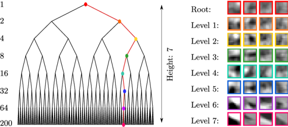
Figure 2: (left) Our obtained search tree (with numbers of nodes for each level). (right) Four patches well represented by each of the eight nodes along the branch highlighted in red in the tree. These patches are randomly sampled from the generative model encoded at each node of the branch (patches on the same column are generated from the same random seed).

As shown in Table I, the step Gaussian selection has a complexity of $\mathcal{O}(NP^{2}K)$, reduced to $\mathcal{O}(NPK\bar{r})$ using the flat tail spectrum approximation. This step remains the biggest bottleneck since each query patch has to be compared to all the $K$ components of the GMM. To make this step even more efficient, we reduce its complexity using a balanced search tree. As described below, such a tree can be built offline by repeatedly collapsing the original GMM to models with fewer components, until the entire model is reduced to a single Gaussian model.

We progressively combine the GMM components from one level to form the level above, by clustering the $K$ components into $L<K$ clusters of similar ones, until the entire model is reduced to a single component. The similarity between two zero-mean Gaussian models with covariance ${\boldsymbol{\Sigma}}_{1}$ and ${\boldsymbol{\Sigma}}_{2}$ is measured by the symmetric Kullback-Leibler (KL) divergence

$$\mathrm{KL}({\boldsymbol{\Sigma}}_{1},{\boldsymbol{\Sigma}}_{2})=\tfrac{1}{2}\operatorname{Tr}({\boldsymbol{\Sigma}}_{2}^{-1}{\boldsymbol{\Sigma}}_{1}+{\boldsymbol{\Sigma}}_{1}^{-1}{\boldsymbol{\Sigma}}_{2}-2\mathrm{Id}_{P}).$$ (17)

Based on this divergence, at each level $n$, we look for a partition $\Omega^{{n}}$ of the $K$ Gaussian components into $L$ clusters (with about equal sizes) minimizing the following optimization problem

$$\underset{\Omega^{{n}}}{\operatorname{argmin}}\;\sum_{l=1}^{L}\sum_{{k_{1},k_{2}\in\Omega_{l}^{{n}}}}\mathrm{KL}({\boldsymbol{\Sigma}}_{k_{1}},{\boldsymbol{\Sigma}}_{k_{1}}),$$ (18)

such that $\bigcup_{l=1}^{L}\Omega_{l}^{{n}}=[K]$ and $\Omega_{l_{1}}^{{n}}\underset{\!l_{1}\neq l_{2}\!}{\cap}\Omega_{l_{2}}^{{n}}=\emptyset$, where $\Omega_{l}^{{n}}$ is the $l$-th set of Gaussian components for the GMM at level $n$. This clustering problem can be approximately solved using the genetic algorithm of [22] for the Multiple Traveling Salesmen Problem (MTSP). MTSP is a variation of the classical Traveling Salesman Problem where several salesmen visit a unique set of cities and return to their origins, and each city is visited by exactly one salesman. This attempts to minimize the total distance traveled by all salesmen. Hence, it is similar to our original problem given in eq. (18) where the Gaussian components and the clusters correspond to $K$ cities and $L$ salesmen, respectively. Given the clustering at level $n$, the new GMM at level $n-1$ is obtained by combining the zero-mean Gaussian components such that, for all $1\leqslant l\leqslant L$:

$$w_{l}^{{n-1}}=\sum\limits_{k\in\Omega_{l}^{{n}}}w_{k}^{{n}}\quad\text{and}\quad{\boldsymbol{\Sigma}}_{l}^{{n-1}}=\frac{1}{w_{l}^{{n-1}}}\sum\limits_{k\in\Omega_{l}^{{n}}}w_{k}^{{n}}{\boldsymbol{\Sigma}}_{k}^{{n}},$$ (19)

where ${\boldsymbol{\Sigma}}^{{n}}_{k}$ and $w^{{n}}_{k}$ are the corresponding covariance matrix and weight of the $k$-th Gaussian component at level $n$. Following this scheme, the original GMM of $K\!=\!200$ components is collapsed into increasingly more compact GMMs with $K\!=\!64$, $32$, $16$, $8$, $4$, $2$ and $1$ components. The main advantage of using MTSP compared to classical clustering approaches, is that this procedure can be adapted easily to enforce approximately equal sized clusters, simply by enforcing that each salesman visits at least $3$ cities for the last level and $2$ for the other ones.

We also experimented with other clustering strategies such as the hierarchical kmeans-like clustering in [17] and hierarchical agglomerative clustering. With no principled way to enforce even-sized clusters, these approaches, in general, lead to unbalanced trees (with comb structured branches) which result in large variations in computation times from one image to another. Although they all lead to similar denoising performances, we opted for MTSP based clustering to build our Gaussian tree in favor of obtaining a stable speed-up profile for our resulting algorithm.

In Fig. 2 we show that the tree obtained using MTSP-based clustering is almost a binary tree (left) and also display the types of patches it encodes along a given path (right). Such a balanced tree structure lets one avoid testing each patch against all $K$ components. Instead, a patch is first compared to the two first nodes in level 1 of the tree, then the branch providing the smallest cost is followed and the operation is repeated at higher levels until a leaf has been reached. Using this balanced search tree reduces the complexity of step Gaussian selection to $\mathcal{O}(NP\bar{r}\log K)$.

III-C Speed-up via the restriction to a random subset of patches

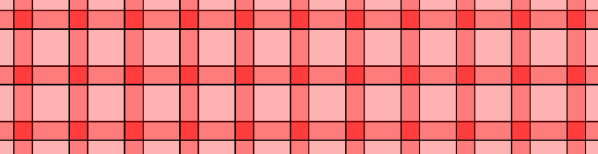
(a) Regular patch subsampling at $(i_{0},j_{0})$

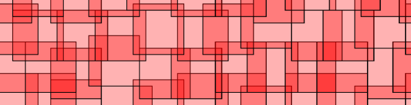
(b) Stochastic patch subsampling at $(i,j)$

Figure 3: Illustration of patch subsampling. Instead of extracting all patches, only a subset of patches is extracted either (a) regularly or (b) with some randomizations. Patches are represented by $8\!\times\!8$ squares and the red intensity represents the number of patches overlapping the corresponding pixel.

The simplest and most effective proposed acceleration consists of subsampling the set $\mathcal{I}$ of $N$ patches to improve the complexity of the four most time-consuming steps, see Table I. One approach, followed by BM3D [8], consists of restricting the set $\mathcal{I}$ to locations on a regular grid with spacing $s\in[1,\sqrt{P}]$ pixels in both directions, leading to a reduction of complexity by a factor $s^{2}$. We refer to this approach as the regular patch subsampling. A direct consequence is that $|\mathcal{I}|\!=\!N/s^{2}$ and the complexity is divided by $s^{2}$. However, we observed that this strategy consistently creates blocky artifacts revealing the regularity of the extraction pattern. A random sampling approach, called "jittering", used in the computer graphics community [7] is preferable to limit this effect. This procedure ensures that each pixel is covered by at least one patch. The location $(i_{0},j_{0})$ of a point of the grid undergoes a random perturbation, giving a new location $(i,j)$ such that

$$i_{0}-\left\lfloor\tfrac{\sqrt{P}-s}{2}\right\rfloor\leqslant i\leqslant i_{0}+\left\lfloor\tfrac{\sqrt{P}-s}{2}\right\rfloor$$

and $$j_{0}-\left\lfloor\tfrac{\sqrt{P}-s}{2}\right\rfloor\leqslant j\leqslant j_{0}+\left\lfloor\tfrac{\sqrt{P}-s}{2}\right\rfloor,$$ (20)

where $\lfloor\cdot\rfloor$ denotes the flooring operation. We found experimentally that independent and uniform perturbations offered the best performance against all other tested strategies. In addition, we also resample these positions at each of the $T$ iterations and add a (random) global shift to ensure that all pixels have the same expected number of patches covering them.

Figure 3 illustrates the difference between a regular grid and a jittered grid of period $s\!=\!6$ for patches of size $P\!=\!8\!\times\!8$. In both cases, all pixels are covered by at least one patch, but the stochastic version reveals an irregular pattern.

Nevertheless, when using random subsampling, a major bottleneck occurs when $\mathcal{A}^{t}\mathcal{A}$ is not diagonal because the inversion involved in eq. (6) cannot be simplified as in Alg. 1. Using a conjugate gradient is a practical solution but will negate the reduction of complexity gained by using subsampling. To the best of our knowledge, this is the main reason why patch subsampling has not been utilized to speed up EPLL. Here, we follow a different path. We opt for approximating the solution of the original problem (involving all patches) rather than evaluating the solution of an approximate problem (involving random subsample of patches). More precisely, we speed up Alg. 1 by replacing the complete set of indices by the random subset of patches. In this case, step Patch reprojection consists of averaging only this subset of overlapping restored patches. This novel and nuanced idea avoids additional overhead and attains dramatic complexity improvements compared to the standard approach.

Experiments conducted on our validation dataset show that this strategy used with $s\!=\!6$ leads to an acceleration of about $36\times$ with less than a $0.2$dB drop in PSNR. In comparison, for a similar drop of PSNR, the regular patch subsampling can only achieve a $9\times$ acceleration with $s\!=\!3$.

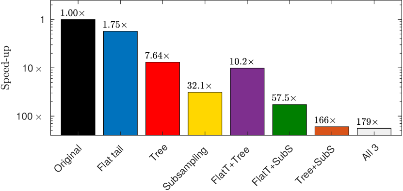
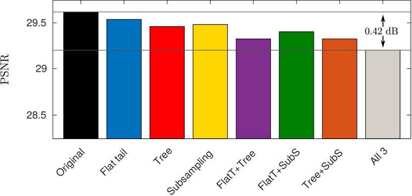
Figure 4: (left) Average speed-up and (right) average PSNR for our three accelerations, and all possible combinations of them, on the $40$ images of the BSDS validation set.

III-D Performance analysis

Figure 4 shows the image restoration performance and speed-up obtained when the three ingredients are applied separately or in combination. The results are averaged over 40 images from the test set of BSDS dataset [28] that is set aside for validation purposes. The speed-up is calculated with respect to the EPLLc implementation which is labeled “original” in Fig. 4. Among the three ingredients, random subsampling or jittering (labeled “subsampling”) leads to the largest speed-up ($32\times$), while the usage of the search tree provides more than $7\times$ faster processing. The average speed-up obtained when combining all three ingredients is around $179\times$ on our validation set consisting of images of size $481\!\times\!321$, for an average drop of PSNR less than $0.5$dB.

IV Related methods

To the best of our knowledge, there are only two other approaches [36, 32] that have attempted to accelerate EPLL. Unlike our approach, these methods focus on accelerating only one of the steps of EPLL namely the Gaussian selection step. Both use machine learning techniques to reduce its runtime.

In [36], the authors use a binary decision tree to approximate the mapping $\tilde{\boldsymbol{z}}_{i}\mapsto k^{*}_{i}$ performed in step Gaussian selection. At each node $k$ and level $n$ of the tree, the patch $\tilde{\boldsymbol{z}}_{i}$ is confronted with a linear separator in order to decide if the recursion should continue on the left or right child given by

$$\langle{\boldsymbol{a}}_{k}^{n},\,\tilde{\boldsymbol{z}}_{i}\rangle+b_{k}^{n}\geqslant 0$$ (21)

where $({\boldsymbol{a}}_{k}^{n},b_{k}^{n})$ are the parameters of the hyperplane for the $k$-th node at level $n$. These separators are trained offline on all pairs of $(\tilde{\boldsymbol{z}}_{i},k^{*}_{i})$ obtained after the first iteration of EPLL for a given $\beta$ and noise level $\sigma$. Once a leaf has been reached, its index provides a first estimate for the index $k^{*}_{i}$. To reduce errors due to large variations among the neighboring pixels, this method further employs a Markov random fields on the resulting map of Gaussian components which runs in $\mathcal{O}(NK)$ complexity. Hence, their overall approach reduces the complexity of step Gaussian selection from $\mathcal{O}(NKP^{2})$ to $\mathcal{O}(N(PD+K))$, where $D=12$ is the depth of the learned decision tree.

TABLE II: PSNR, SSIM and execution time on the BSDS test set (average on 60 images of size $481\!\times\!321$), and on six standard images (each of size $512\!\times\!512$) for the proposed FEPLL and FEPLL^′, EPLL (with timing given for both EPLLm [39] and our EPLLc), BM3D [8], CSF [33] and RoG [32] with 3 different levels of noise.

$\sigma$	Algo.	Berkeley	Barbara	Boat	Couple	Fingerprint	Lena	Mandrill
		PSNR/SSIM
$5$	FEPLL	36.8 / .959	36.9 / .958	36.6 / .930	36.7 / .944	35.4 / .984	38.1 / .941	35.1 / .959
	FEPLL′	37.1 / .962	37.4 / .961	36.8 / .933	37.0 / .948	35.9 / .985	38.4 / .943	35.2 / .960
	EPLL	37.3 / .963	37.6 / .962	36.8 / .933	37.3 / .949	36.5 / .987	38.6 / .944	35.2 / .960
	RoG	37.1 / .959	36.7 / .954	36.5 / .920	37.2 / .946	36.4 / .987	38.3 / .938	35.0 / .956
	BM3D	37.3 / .962	38.3 / .964	37.3 / .939	37.4 / .949	36.5 / .987	38.7 / .944	35.2 / .959
	CSF3×3	36.8 / .952	37.0 / .955	36.7 / .929	37.1 / .945	36.2 / .986	38.2 / .938	34.8 / .953
$20$	FEPLL	29.1 / .812	29.1 / .853	30.1 / .802	29.9 / .812	27.7 / .909	32.3 / .863	26.4 / .786
	FEPLL′	29.3 / .831	29.7 / .869	30.4 / .815	30.2 / .827	28.1 / .920	32.4 / .865	26.6 / .805
	EPLL	29.5 / .836	29.9 / .874	30.6 / .821	30.4 / .833	28.3 / .924	32.6 / .869	26.7 / .808
	RoG	29.3 / .828	28.4 / .838	30.4 / .815	30.2 / .826	28.3 / .922	32.5 / .866	26.5 / .796
	BM3D	29.4 / .824	31.8 / .905	30.8 / .825	30.7 / .842	28.8 / .929	33.0 / .877	26.6 / .796
	CSF3×3	29.0 / .805	28.3 / .822	30.2 / .802	29.9 / .812	28.0 / .917	31.8 / .838	26.1 / .779
$60$	FEPLL	24.5 / .614	23.5 / .634	25.5 / .644	25.0 / .626	22.1 / .721	27.4 / .742	21.4 / .468
	FEPLL′	24.5 / .620	23.8 / .646	25.6 / .646	25.1 / .634	22.4 / .746	27.2 / .729	21.6 / .501
	EPLL	24.8 / .631	24.0 / .658	25.8 / .658	25.3 / .646	22.6 / .754	27.6 / .746	21.7 / .506
	RoG	24.6 / .622	23.3 / .624	25.6 / .653	25.1 / .638	22.4 / .739	27.3 / .744	21.5 / .480
	BM3D	24.8 / .637	26.3 / .756	25.9 / .671	25.5 / .662	23.7 / .800	28.2 / .775	21.7 / .501
	CSF3×3	22.0 / .489	21.4 / .487	22.7 / .504	22.5 / .503	21.2 / .727	23.4 / .509	20.3 / .467
		Time (in seconds)
	FEPLL	000.27	000.42	000.40	000.41	000.38	000.43	000.42
	FEPLL′	000.96	001.91	001.90	001.90	001.90	001.90	001.90
	EPLLc	044.86	078.66	078.71	078.78	078.17	078.13	078.34
	EPLLm	082.68	145.15	143.68	144.30	144.13	144.15	143.86
	RoG	001.19	001.99	001.97	001.96	001.94	001.98	001.96
	BM3D	001.64	002.79	002.91	002.83	002.45	002.87	002.84
	CSF3×3	000.87	001.09	001.09	001.13	001.09	001.09	001.08
	CSF${}_{3\times 3}^{\text{gpu}}$	000.41	000.41	000.41	000.41	000.41	000.40	000.41

In [32], the authors approximate the Gaussian selection step, by using a gating (feed-forward) network with one hidden layer

$$\tilde{\boldsymbol{z}}_{i}\mapsto\iota^{k}\!+\!\sum_{j=1}^{Q}\biggl{(}\log\nu^{k}_{j}\!+\!\omega^{k}_{j}(\tilde{\boldsymbol{d}}_{i})_{j}^{2}\biggr{)}\quad\text{with}\quad\tilde{\boldsymbol{d}}_{i}={\boldsymbol{V}}^{t}\tilde{\boldsymbol{z}}_{i}$$ (22)

where $Q$ is the size of the hidden layer. The matrix ${\boldsymbol{V}}\in\mathbb{R}^{P\times Q}$ encodes the weights of the first layer, $\omega^{k}$ corresponds to the weights of the hidden layer and they are learned discriminatively to approximate the exact posterior probability:

$$\tilde{\boldsymbol{z}}_{i}\mapsto\iota^{k}\!+\!\sum_{j=1}^{P}\biggl{(}\log\nu^{k}_{j}\!+\!\frac{(\tilde{\boldsymbol{c}}_{i}^{k})_{j}^{2}}{\nu^{k}_{j}}\biggr{)}\quad\text{with}\quad\tilde{\boldsymbol{c}}_{i}^{k}={\boldsymbol{U}}_{k}^{t}\tilde{\boldsymbol{z}}_{i}$$ (23)

that we encounter in eq. (7) and (8). Theoretically, a new network will need to be trained for each type of degradations, noise levels and choices of $\beta$ (recall that $\nu^{k}_{j}=({\boldsymbol{S}}_{k})_{jj}+\frac{1}{\beta}$). However, the findings of [32] indicate that applying a network learned on clean patches and with $\frac{1}{\beta}=0$ is effective regardless of the type of degradation or the value of $\beta$. Their main advantage can be highlighted by comparing eq. (22) and (23) where complexity is reduced from $\mathcal{O}(NKP^{2})$ to $\mathcal{O}(NQ(K+P))$. The authors utilize this benefit by choosing $Q=100$.

Unlike these two approaches, our method does not try to learn the Gaussian selection rule directly (which depends on both the noise level through $1/\beta$ and the prior model through the GMM). Instead, we simply define a hierarchical organization of the covariance matrices ${\boldsymbol{\Sigma}}_{k}$. In other words, while the two other approaches try to infer the posterior probabilities (or directly the maximum a posteriori), our approach provides an approximation to the prior model. During runtime, this approximation of the prior is used in the posterior for the Gaussian selection task. Please note that the value of $\beta$ does not play a role in determining the prior. This allows us to use the same search tree independently of the noise level, degradations, etc. Given that the main advantage of EPLL is that the same model can be used for any type of degradations, it is important that this property remains true for the accelerated version. Last but not least, the training of our search tree takes a few minutes while the training steps for the above mentioned approach take from several hours to a few days [36].

In the next section, we show that our proposed accelerations produce restoration results with comparable quality to competing methods while requiring a smaller amount of time.

V Numerical experiments

In this section, we present the results obtained on various image restoration tasks. Our experiments were conducted on standard images of size $512\times 512$ such as Barbara, Boat, Couple, Fingerprint, Lena, Mandrill and on 60 test images of size $481\!\times\!321$ from the Berkeley Segmentation Dataset (BSDS) [28] (the original BSDS test set contains 100 images, the other 40 was used for validation purposes while setting parameters $\rho$ and $s$). For denoising, we compare the performance of our fast EPLL (FEPLL) to the original EPLL algorithm [39] and BM3D [8]. For the original EPLL, we have included timing results given by our own MATLAB/C implementation (EPLLc) and the MATLAB implementation provided by the authors (EPLLm). We also compare our restoration performance and runtime against other fast restoration methods introduced to achieve competitive trade-off between runtime efficiency and image quality. These methods include RoG [32] (a method accelerating EPLL based on feedforward networks described in Sec. IV), and CSF [33] (a fast restoration technique using random field-based architecture).

For deblurring experiments, we additionally compare with field-of-experts (FoE)-based non-blind deconvolution [5] denoted as iPiano. We contacted the corresponding author of [36] and got confirmation that the implementation of their algorithm (briefly described in IV) is not publicly available. Due to certain missing technical details, we were unable to reimplement it faithfully. However, the results reported in [36] indicate that their algorithm performs in par with BM3D in terms of both PSNR and time. Hence, BM3D results can be used as a faithful proxy for the expected performance of Wang et al.’s algorithm [36].

To explicitly illustrate the quality vs. runtime tradeoff of FEPLL, we include results obtained using a slightly slower version of FEPLL referred to as FEPLL^′, that does not use the balanced search tree and uses a flat tail spectrum approximation with $\rho=0.98$. Please note that FEPLL^′ is not meant to be better or worse than FEPLL, it is just another version running at a different PSNR/time tradeoff which allows us to compare our algorithm to others operating in different playing fields.

Finally, to illustrate the versatility of FEPLL, we also include results for other inverse problems such as devignetting, super-resolution, and inpainting.

(a) Reference ${\boldsymbol{x}}$

$\bf 22.1$ / $\bf.368$

(b) Noisy image ${\boldsymbol{y}}$

$\bf 30.6$ / $\bf.872$ ($\bf 1.68$s)

(c) BM3D result $\hat{\boldsymbol{x}}$

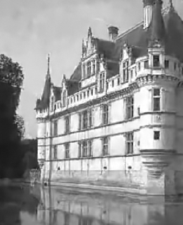
$\bf 30.6$ / $\bf.873$ ($\bf 44.88$s)

(d) EPLLc result $\hat{\boldsymbol{x}}$

$\bf 30.2$ / $\bf.862$ ($\bf 0.36$s)

(e) FEPLL result $\hat{\boldsymbol{x}}$

Figure 5: Illustration of a denoising problem with noise standard deviation $\sigma=20$. Part of: (a) the original image (b) its noisy version (c-e) denoised results of competitive methods with PSNR/SSIM and time (inset).

Parameter settings

In our experiments, we use patches of size $P\!=\!8\!\times\!8$, and the GMM provided by Zoran et al. [39] with $K\!=\!200$ components. The 200-components GMM is progressively collapsed into smaller GMMs with $K\!=\!64,32,16,8,4,2$ and $1$, and then all Gaussians of the tree are modified offline by flat-tail approximations with $\rho\!=\!0.95$. The final estimate for the restored image is obtained after 5 iterations of our algorithm with $\beta$ set to ${\lambda}{\sigma^{-2}}\{1,4,8,16,32\}$ where $\lambda\!=\!\min\{N^{-1}{|\!|\mathcal{A}^{t}\mathcal{A}|\!|_{F}^{2}}{|\!|\mathcal{A}|\!|^{-2}_{2}},250\sigma^{2}\}$. For denoising, where $\mathcal{A}$ is identity, $\lambda\!=\!1$ which boils down to the setting used by Zoran et al. [39]. For inverse problems, we found that the initialization $\hat{\boldsymbol{x}}=(\mathcal{A}^{t}\mathcal{A}+0.2\sigma^{2}/\lambda\nabla)^{-1}\mathcal{A}^{t}{\boldsymbol{y}}$, with $\nabla$ the image Laplacian, provides relevant solutions whatever the linear operator $\mathcal{A}$ and the noise level $\sigma^{2}$. While the authors of [39] do not provide any further direction for setting $\beta$ and the initialization in general inverse problems, our proposed setting leads to competitive solutions irrespective of $\mathcal{A}$ and $\sigma^{2}$. For BM3D [8], EPLLm [39], RoG [32], CSF [33] and iPiano [5] we use the implementations provided by the original authors and use the default parameters prescribed by them.

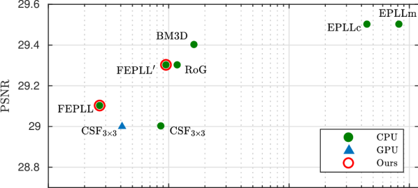
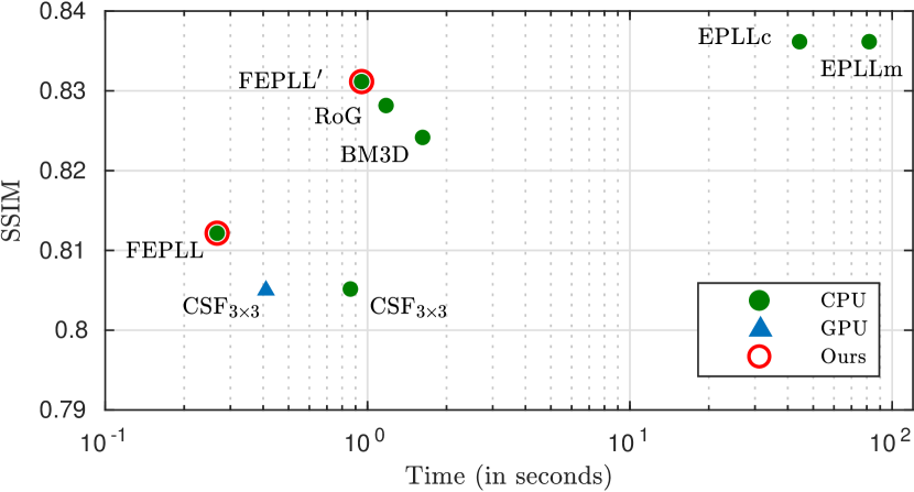
Figure 6: (a) PSNR and (b) SSIM versus time for different restoration methods in a denoising problem with noise standard deviation $\sigma=20$. PSNR, SSIM and time are averaged on the 60 BSDS test images, each of size $481\times 321$. Optimal methods tend to be in the top-left corner.

Denoising

Table II shows the quantitative performances of FEPLL on the denoising task compared to EPLLm [39], EPLLc (our own MATLAB/C implementation), RoG [32] BM3D [8] and CSF [33]. We evaluate the algorithms under low-, mid- and high-noise settings by using Gaussian noise of variance $5^{2}$, $20^{2}$ and $60^{2}$, respectively. The result labeled “Berkeley” is an average over 60 images from the BSDS testing set [28]. Figures 6 provide graphical representations of these performances in terms of PSNR/SSIM versus computation time for the BSDS images for the noise variance setting $\sigma^{2}=20^{2}$. On average, FEPLL results are 0.5dB below regular EPLL and BM3D; however, FEPLL is approximately 7 times faster than BM3D, 170-200 times faster than EPLLc and over 350 times faster than EPLLm. FEPLL outperforms the faster CSF algorithm in terms of both PSNR and time. In this case, FEPLL is even faster than the GPU accelerated version of CSF (CSF${}_{\text{gpu}}$). Our approach is 4 times faster than RoG with a PSNR drop of 0.1-0.3dB. Nevertheless, if we slow down FEPLL to FEPLL^′, we can easily neutralize this quality deficit while still being faster than RoG. Note that these accelerations are obtained purely based on the approximations and no parallel processing is used. Also, in most cases, a loss of 0.5dB may not affect the visual quality of the image. To illustrate this, we show a sample image denoised by BM3D, EPLL and FEPLL in Fig. 5.

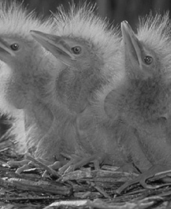
(a) Reference ${\boldsymbol{x}}$ / Blur kernel

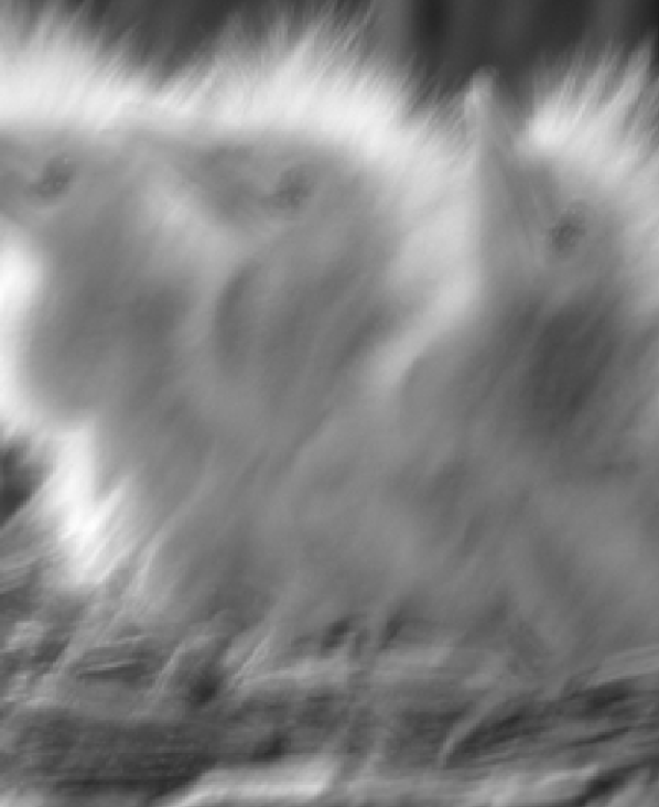
$\bf 24.9$ / $\bf.624$

(b) Blurry image ${\boldsymbol{y}}$

$\bf 31.4$ / $\bf.891$ ($\bf 0.17*$s)

(c) CSF_pw result $\hat{\boldsymbol{x}}$

$\bf 32.2$ / $\bf.910$ ($\bf 1.17$s)

(d) RoG result $\hat{\boldsymbol{x}}$

$\bf 32.7$ / $\bf.924$ ($\bf 0.46$s)

(e) FEPLL result $\hat{\boldsymbol{x}}$

Figure 7: Illustration of a deblurring problem with noise standard deviation $\sigma=0.5$. Part of: (a) the original image and the blur kernel (inset), (b) blurry version (c-e) deblurred results of competitive methods with PSNR/SSIM and time (inset). The ’*’ indicates runtime on GPU while others are CPU times.

Deblurring

Table III shows the performance of FEPLL when used for deblurring as compared to RoG [32], iPiano [5] and CSF [33]. For these experiments, we use the blur kernel provided by Chen et al. [5] along with their algorithm implementation. The results under the label “Berkeley” are averaged over 60 images from the BSDS test dataset [28]. The results labeled “Classic” is averaged over the six standard images (Barbara, Boat, Couple, Fingerprint, Lena and Mandrill). FEPLL consistently outperforms its efficient competitors both in terms of quality and runtime. Although the GPU version of CSF is faster, the restoration quality obtained by CSF is 2-3dB lower than FEPLL. The proposed algorithm outperforms RoG by 1-1.8dB while running 3 and 5 times faster on “Berkeley” and “Classic” datasets, respectively.

The superior qualitative performance of FEPLL is demonstrated in Fig. 7. For brevity, we only include the deblurring results obtained from the top competitors of FEPLL algorithm in terms of both quality and runtime. As observed, FEPLL provides the best quality vs. runtime efficiency trade-off. In contrast, a deblurring procedure using the regular EPLL is around 350 times slower than FEPLL with the original implementation [39]. Specifically, on the sample image shown in Fig. 7, EPLL provides a qualitatively similar result (not shown in the figure) with a PSNR of 32.7 dB and SSIM of 0.922 in 142 seconds.

Other inverse problems

Unlike BM3D, EPLL and FEPLL are more versatile and handle a wide range of inverse problems without any change in formulation. In Fig. 8, we show the results obtained by FEPLL on problems such as (a) devignetting, which involves a progressive loss of intensity, (b) super-resolution and (c) inpainting. To show the robustness of our method, the input images of size $481\!\times\!321$ were degraded with zero-mean Gaussian noise with $\sigma\!=\!2$. All of the restoration results were obtained within/under 0.4 seconds and with the same set of parameters explained above (cf. Parameter settings).

TABLE III: PSNR, SSIM and execution time on the BSDS test set (average of 60 images of size $481\!\times\!321$), and on standard images (average of 6 images of size $512\!\times\!512$) for the proposed FEPLL and FEPLL^′, CSF [33], RoG [32] and Chen et al.’s [5] method that is called iPiano in their implementation. The blur kernel used is the one provided in along with iPiano implementation and noise is set to $\sigma=0.5$.

Algo.	Berkeley		Classic
	PSNR/SSIM	Time (s)	PSNR/SSIM	Time (s)
iPiano	29.5 / .824	29.53	29.9 / .848	59.10
CSF${}_{\text{pw}}$	30.2 / .875	0.50 (0.14*)	30.5 / 0.870	0.47 (0.14*)
RoG	31.3 / .897	1.19	31.8 / .915	2.07
FEPLL	33.1 / .928	0.40	32.8 / .931	0.46
FEPLL’	33.2 / .930	1.01	33.0 / .933	1.82

VI Conclusion

In this paper, we accelerate EPLL by a factor greater than 100 with negligible loss of image quality (less than $0.5$dB). This is achieved by combining three independent strategies: a flat tail approximation, matching via a balanced search tree, and stochastic patch sampling. We show that the proposed accelerations are effective in denoising and deblurring problems, as well as in other inverse problems such as super-resolution and devignetting. An important distinction of the proposed accelerations is their genericity: the accelerated EPLL prior can be applied to many restoration tasks and various signal-to-noise ratios, in contrast to existing accelerations based on learning techniques applied to specific conditions (such as image size, noise level, blur kernel, etc.) and that require an expensive re-training to address a different problem.

Since the speed-up is achieved solely by reducing the algorithmic complexity, we believe that further inclusion of accelerations based on parallelization and/or GPU implementations will allow for real-time video processing. Moreover, the acceleration techniques introduced in this work are general strategies that can be used to speed up other image restoration and/or related machine learning algorithms. For reproducibility purposes, the code of FEPLL is made available on GitHub.

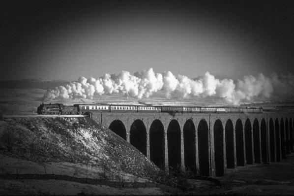
$\bf 11.1$ / $\bf.662$

$\bf 20.8$ / $\bf.598$

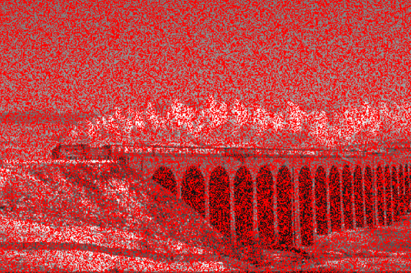
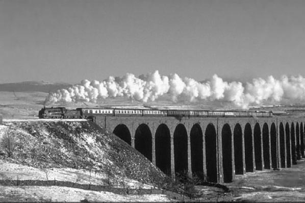
$\bf 8.31$ / $\bf.112$ $\bf 36.8$ / $\bf.972$ ($\bf 0.38$s) (a) devignetting $\bf 23.3$ / $\bf.738$ ($\bf 0.29$s) (b) $\times 3$ super-resolution $\bf 27.0$ / $\bf.905$ ($\bf 0.36$s) (c) $50$% inpainting

Figure 8: FEPLL on various inverse problems. All inputs contain Gaussian noise with $\sigma=2$. Top row: (a) the observation in a devignetting problem, (b) the bi-cubic interpolation and the actual low-resolution size image (inset) in a $\times 3$ super-resolution problem and (c) the observation in an inpainting problem with $50\%$ of missing pixels shown in red. Bottom row: respective FEPLL results all obtained in less than $0.4$s.

References

- [1] M. Aharon, M. Elad, and A. Bruckstein. k -svd: An algorithm for designing overcomplete dictionaries for sparse representation. IEEE Transactions on Signal Processing, 54(11):4311–4322, Nov 2006.
- [2] A. Buades, B. Coll, and J.-M. Morel. A review of image denoising algorithms, with a new one. Multiscale Modeling & Simulation, 4(2):490–530, 2005.
- [3] H. Burger, C. Schuler, and S. Harmeling. Image denoising: Can plain neural networks compete with BM3D? In International Conference on Computer Vision and Pattern Recognition (CVPR), 2012.
- [4] N. Cai, Y. Zhou, S. Wang, B. W.-K. Ling, and S. Weng. Image denoising via patch-based adaptive gaussian mixture prior method. Signal, Image and Video Processing, 10(6):993–999, 2016.
- [5] Y. Chen, R. Ranftl, and T. Pock. Insights into analysis operator learning: From patch-based sparse models to higher order mrfs. IEEE Transactions on Image Processing, 23(3):1060–1072, March 2014.
- [6] Y. Chen, W. Yu, and T. Pock. On learning optimized reaction diffusion processes for effective image restoration. In Proceedings of the IEEE Conference on Computer Vision and Pattern Recognition, pages 5261–5269, 2015.
- [7] R. L. Cook. Stochastic sampling in computer graphics. ACM Transactions on Graphics (TOG), 5(1):51–72, 1986.
- [8] K. Dabov, A. Foi, V. Katkovnik, and K. Egiazarian. Image denoising by sparse 3-D transform-domain collaborative filtering. IEEE Transactions on Image Processing, 16(8):2080–2095, August 2007.
- [9] A. Danielyan, A. Foi, V. Katkovnik, and K. Egiazarian. Image upsampling via spatially adaptive block-matching filtering. In Signal Processing Conference, 2008 16th European, pages 1–5. IEEE, 2008.
- [10] A. Danielyan, A. Foi, V. Katkovnik, and K. Egiazarian. Spatially adaptive filtering as regularization in inverse imaging: Compressive sensing super-resolution and upsampling. Super-Resolution Imaging, pages 123–154, 2010.
- [11] C.-A. Deledalle, J. Salmon, and A. S. Dalalyan. Image denoising with patch based PCA: local versus global. In BMVC 2011-22nd British Machine Vision Conference, pages 25–1. BMVA Press, 2011.
- [12] A. P. Dempster, N. M. Laird, and D. B. Rubin. Maximum likelihood from incomplete data via the EM algorithm. Journal of the royal statistical society. Series B (methodological), pages 1–38, 1977.
- [13] C. Dong, C. C. Loy, K. He, and X. Tang. Image super-resolution using deep convolutional networks. IEEE transactions on pattern analysis and machine intelligence, 38(2):295–307, 2016.
- [14] K. Egiazarian and V. Katkovnik. Single image super-resolution via BM3D sparse coding. In Signal Processing Conference (EUSIPCO), 2015 23rd European, pages 2849–2853. IEEE, 2015.
- [15] D. Geman and C. Yang. Nonlinear image recovery with half-quadratic regularization. IEEE Transactions on Image Processing, 4(7):932–946, 1995.
- [16] D. Glasner, S. Bagon, and M. Irani. Super-resolution from a single image. In IEEE 12th International Conference on Computer Vision, 2009.
- [17] J. Goldberger and S. T. Roweis. Hierarchical clustering of a mixture model. In NIPS, volume 17, pages 505–512, 2004.
- [18] A. Houdard, C. Bouveyron, and J. Delon. High-Dimensional Mixture Models For Unsupervised Image Denoising (HDMI). Preprint hal-01544249, Aug. 2017.
- [19] J. Jancsary, S. Nowozin, and C. Rother. Regression tree fields – an efficient, non-parametric approach to image labeling problems. In 25th IEEE Conference on Computer Vision and Pattern Recognition (CVPR), 2012.
- [20] V. Katkovnik and K. Egiazarian. Nonlocal image deblurring: Variational formulation with nonlocal collaborative L0-norm prior. In Local and Non-Local Approximation in Image Processing, 2009. LNLA 2009. International Workshop on, pages 46–53. IEEE, 2009.
- [21] J. Kim, J. Kwon Lee, and K. Mu Lee. Accurate image super-resolution using very deep convolutional networks. In Proceedings of the IEEE Conference on Computer Vision and Pattern Recognition, pages 1646–1654, 2016.
- [22] J. Kirk. Source code for "multiple traveling salesmen problem - genetic algorithm", https://fr.mathworks.com/matlabcentral/fileexchange/19049-multiple-traveling-salesmen-problem-genetic-algorithm. MATLAB Central File Exchange. Retrieved May 6, 2014, 2008.
- [23] D. Krishnan and R. Fergus. Fast image deconvolution using hyper-laplacian priors. In Advances in Neural Information Processing Systems, pages 1033–1041, 2009.
- [24] M. Lebrun, A. Buades, and J.-M. Morel. A nonlocal bayesian image denoising algorithm. SIAM Journal on Imaging Sciences, 6(3):1665–1688, 2013.
- [25] E. López-Rubio. Superresolution from a single noisy image by the median filter transform. SIAM Journal on Imaging Sciences, 9(1):82–115, 2016.
- [26] E. Luo, S. H. Chan, and T. Q. Nguyen. Adaptive image denoising by mixture adaptation. IEEE Transactions on Image Processing, 25(10):4489–4503, 2016.
- [27] J. Mairal, F. Bach, and J. Ponce. Task-driven dictionary learning. IEEE Transactions on Pattern Analysis and Machine Intelligence, 34(4):791–804, 2012.
- [28] D. Martin, C. Fowlkes, D. Tal, and J. Malik. A database of human segmented natural images and its application to evaluating segmentation algorithms and measuring ecological statistics. In Computer Vision, 2001. ICCV 2001. Proceedings. Eighth IEEE International Conference on, volume 2, pages 416–423. IEEE, 2001.
- [29] V. Papyan and M. Elad. Multi-scale patch-based image restoration. IEEE Transactions on image processing, 25(1):249–261, 2016.
- [30] M. Protter, M. Elad, H. Takeda, and P. Milanfar. Generalizing the nonlocal-means to super-resolution reconstruction. IEEE Transactions on image processing, 18(1):36–51, 2009.
- [31] Y. Ren, Y. Romano, and M. Elad. Example-based image synthesis via randomized patch-matching. arXiv preprint arXiv:1609.07370, 2016.
- [32] D. Rosenbaum and Y. Weiss. The return of the gating network: combining generative models and discriminative training in natural image priors. In Advances in Neural Information Processing Systems, pages 2683–2691, 2015.
- [33] U. Schmidt and S. Roth. Shrinkage fields for effective image restoration. In Proceedings of the IEEE Conference on Computer Vision and Pattern Recognition, pages 2774–2781, 2014.
- [34] A. Singh, F. Porikli, and N. Ahuja. Super-resolving noisy images. In Proceedings of the IEEE Conference on Computer Vision and Pattern Recognition, pages 2846–2853, 2014.
- [35] J. Sulam and M. Elad. Expected patch log likelihood with a sparse prior. In International Workshop on Energy Minimization Methods in Computer Vision and Pattern Recognition, pages 99–111. Springer, 2015.
- [36] Y. Wang, S. Cho, J. Wang, and S.-F. Chang. Discriminative indexing for probabilistic image patch priors. In European Conference on Computer Vision, pages 200–214. Springer, 2014.
- [37] G. Yu, G. Sapiro, and S. Mallat. Solving inverse problems with piecewise linear estimators: From gaussian mixture models to structured sparsity. IEEE Transactions on Image Processing, 21(5):2481–2499, 2012.
- [38] K. Zhang, W. Zuo, Y. Chen, D. Meng, and L. Zhang. Beyond a Gaussian Denoiser: Residual Learning of Deep CNN for Image Denoising. arXiv preprint arXiv:1608.03981, 2016.
- [39] D. Zoran and Y. Weiss. From learning models of natural image patches to whole image restoration. In International Conference on Computer Vision, pages 479–486. IEEE, November 2011.