A semi-parametric estimation for max-mixture spatial processes

Abstract.

We propose a semi-parametric estimation procedure in order to estimate the parameters of a max-mixture model as an alternative to composite likelihood estimation. This procedure uses the F-madogram. We propose to minimize the square difference between the theoretical F-madogram and an empirical one. We evaluate the performance of this estimator through a simulation study and we compare our method to composite likelihood estimation. We apply our estimation procedure to daily rainfall data from East Australia.

1. Introduction

One of the main characteristic of environmental or climatic data is their spatial dependence. The dependencies may be strong even for large distances as observed for heat waves or they may be strong at short distances and weak at larger distances, as observed for cevenol rainfall events. Many dependence structures may arise, for example, asymptotic dependence, asymptotic independence, or both. Max-mixture models as defined in [wadsworth2012dependence] are a mixture between a max-stable process and an Asymptotic Independent (AI) process. These kind of models may be useful to fit e.g. rainfall data (see [bacro2016flexible]).

The estimation of the parameters of these processes remains challenging. The usual way to estimate parameters in spatial contexts is to maximize the composite likelihood. For example, in [padoan2010likelihood], [davison2012geostatistics] and many others, the composite likelihood maximization is used to estimate the parameters of max-stable processes. In [bacro2016flexible] and [wadsworth2012dependence], it is used to estimate the parameters of max-mixture processes. Nevertheless, the estimation remains unsatisfactory in some cases as it seems to have difficulties estimating the AI part. So that, an alternative should be welcomed.
We propose a semi-parametric estimation procedure as an alternative to composite likelihood maximization for max-mixture processes. Our procedure is a least square method on the $F$-madogram. That is, we minimize the squared difference between the theoretical $F$-madogram and the empirical one. Some of literature deals with semi-parametric estimation in modeling spatial extremes. For example, [northrop2015efficient] and [aghakouchak2010semi] provided semi-parametric estimators of extremal indexes. In [buhl2016Semiparametric], another semi-parametric procedure to estimate model parameters is introduced. It is based a non linear least square method based on the extremogram for isotropic space-time Browen-Resnick max-stable processes. The semi-parametric procedure that we propose in this study is close to that article.

Section 2 is dedicated to the main tools used in this study; it contains definitions of some spatial dependence measures and of different dependence structures (asymptotic dependence/independence and mixture of them). In Section 3, we calculate an expression for the $F$-madogram of max-mixture models. Section 4 is devoted to estimation procedures of the parameters of max-mixture processes. We prove that our least square-madogram estimation is consistent, provided that the parameters are identified by the $F$-madogram. In Section 5, simulation study is conducted, it allows us to evaluatere the performance of the estimation procedure. Section 6 is devoted to an application on rainfall real data from East Australia. Finally, concluding remarks are discussed in Section 7.

2. Main tools used in the study

Throughout this study, the spatial process $X:=\{X(s),s\in\mathbb{S}\},\mathbb{S}\in\mathbb{R}^{d}$ is assumed to be strongly stationary and isotopic. We recall some basic facts and definitions related to spatial extreme theory.

2.1. Dependence measures

The extremal dependence behavior of spatial processes may be described by several coefficient / measures.
The upper tail dependence coefficient $\chi$ (see[bacro2013measuring, sibuya1959bivariate]) is defined for a stationary spatial process $X$ on $\mathbb{S}\subset\mathbb{R}^{2}$ with margin $F$ by:

(2.1) $$\chi(h)=\lim_{u\to 1^{-}}\mathbb{P}\big{(}F(X(s+h))>u|F(X(s))>u\big{)}\/.$$

The process is said AI (resp. AD) if for all $h\in\mathbb{S}$ $\chi(h)=0$ (resp. $\chi(h)\neq 0$).

For any $h$ the coefficient $\chi(h)$ can alternatively be expressed as the limit when $u\to 1^{-}$ of the function defined on $\mathbb{S}\times[0,1]$ into $[0,1]$, by

(2.2) $$\chi(h,u)=2-\frac{\log\mathbb{P}\big{(}F(X(s))<u,F(X(t))<u\big{)}}{\log\mathbb{P}\big{(}F(X(s))<u\big{)}},\textnormal{for }h\in\mathbb{S},u\in[0,1[.$$

Such that, $\chi(h)=\lim_{u\to^{-}1}\chi(h,u)$.

For AI processes, $\chi$ cannot reveal the strength of the dependence. This is why the authors in [coles1999dependence], introduced an alternative dependance coefficient called lower tail dependence coefficient $\overline{\chi}$. Consider for any $(s,s+h)\in\mathbb{S}^{2}$

(2.3) $$\overline{\chi}(h,u)=\frac{2\log\mathbb{P}\big{(}F(X(s))>u\big{)}}{\log\mathbb{P}\big{(}F(X(s))>u,F(X(s+h))>u\big{)}}-1,\quad 0\leq u\leq 1$$

and $\overline{\chi}(h)=\lim_{u\to 1}\overline{\chi}(h,u)$.

If $\overline{\chi}(h)=1$ for all $h$, the spatial process is asymptotically dependent. Otherwise, the process is asymptotically independent. Furthermore, if $\overline{\chi}\in]0,1[$ ( resp. $]-1,0[$) the locations $s$ and $s+h$ (for any $s$) are asymptotically positively associated (resp. asymptotically negatively associated).

Another important measure of dependence is the extremal coefficient which was introduced by [buishand1984bivariate, schlather2003dependence].For any $s\in\mathbb{S}$ and $s+h\in\mathbb{S}$ and $x\in\mathbb{R}$, let

$$\theta_{F}(h,x)=\frac{\log(P(X(s)<x,X(s+h)<x))}{\log(P(X(s)<x))}.$$

$\theta_{F}$ is related with the upper tail dependence parameter; indeed if $\lim_{x\rightarrow x_{F}}\theta_{F}(h,x)=\theta(h)$ exists, we have the following relation (see [bacro2013measuring]):

$$\chi(h)=2-\theta_{F}(h),$$

where $x_{F}=\sup\{x|F(x)<1\}$. In that case, $P(X(s)<x,X(s+h)<x))$ may be approximated by $F(x)^{\theta_{F}(h)}$ for $x$ large.

This coefficient is particularly useful when dealing with asymptotic dependence, but useless in case of asymptotic independence. To overcome this problem, [ledford1996statistics] proposed a model allowing to gather all the different dependence behaviors. This model has Fréchet marginal laws and for all $(s,s+h)\in\mathbb{S}^{2}$ the pairwise survivor function is given by:

(2.4) $$\mathbb{P}\big{(}X(s)>x,X(s+h)>x\big{)}=\mathcal{L}_{h}(x)x^{-1/\eta(h)},\quad\textnormal{ as }x\to\infty\/,$$

where $\mathcal{L}_{h}$ is a slowly varying function and $\eta(h)\in(0,1]$ is the tail dependence coefficient. This coefficient determines the decay rate of the bivariate tail probability for large $x$. The interest of this simple modelization, which appears to be quite general, is that the coefficient $\eta(h)$ provides a measure of the extremal dependence between $X(s)$ and $X(x+h)$.
$\mathcal{L}(x)\not\to 0$ (resp. $0<\eta(h)<1$ and $\mathcal{L}(x)\not\to 0$), corresponds to asymptotic dependence (resp. asymptotic independence); see [bacro2013measuring, ledford1996statistics]. Finally, it is important to see the relation between $\eta$ and $\overline{\chi}$. If equation (2.4) is satisfied, then $\overline{\chi}(h)=2\eta(h)-1$.

Another classical tool often used in geostatistics is the variogram. But for spatial processes with Fréchet marginal laws, the variogram does not exist. We shall use the $F$-madogram introduced in [cooley2006variograms] which is defined for any spatial process $X$ with univariate margin $F$ and for all $(s,t)\in\mathbb{S}^{2}$

(2.5) $$\nu^{F}(s-t)=\frac{1}{2}\mathbb{E}|F(X(s))-F(X(t))|.$$

2.2. Spatial extreme models

For completeness, we recall definitions on max-stable, inverse max-stable and max-mixture processes.

2.3. Max-stable model

Max-stable processes are the extension of the multivariate extreme value theory to the infinite dimensional setting [buhl2016Semiparametric]. If there exist two sequences of continuous functions $(a_{n}(\cdot)>0,n\in\mathbb{N})$ and $(b_{n}(\cdot)\in\mathbb{R},n\in\mathbb{N})$ such that for all $n\in\mathbb{N}$ and $n$ i.i.d. $X_{1},\ldots,X_{n}$ and $X$ a process, such that

(2.6) $$\max_{i=1,...,n}\frac{X_{i}-b_{n}}{a_{n}}\stackrel{{\scriptstyle d}}{{\to}}X,\quad n\to\infty,$$

then $X:=\{X(s),s\in\mathbb{S}\}$ is a max-stable process [de2006spatial]. When for all $n\in\mathbb{N}$, $a_{n}=1$ and $b_{n}=0$, the margin distribution of the process $X$ is unit Fréchet, that is for any $s\in\mathbb{S}$ and $x>0$,

$$F(x):=P(X(s)\leq x)=\exp[-1/x]\/,$$

in that case, we say that $X$ is a simple max-stable porcess.
In [de1984spectral] it is proved that a max-stable process $X$ can be constructed by using a random process and a Poisson process. This representation is named the spectral representation. Let $X$ be a max-stable process on $\mathbb{S}$. Then there exists $\{\xi_{i},i\geq 1\}$ i.i.d Poisson point process on $(0,\infty)$, with intensity $d\xi/\xi^{2}$ and a sequence $\{W_{i},i\geq 1\}$ of i.i.d. copies of a positive process $W=(W(s),s\in\mathbb{S})$, such that $\mathbb{E}[W(s)]=1$ for all $s\in\mathbb{S}$ such that

(2.7) $$X=^{d}\max_{i\geq 1}\xi_{i}W_{i}\/.$$

The c.d.f. of a simple max-stable process satisfies: (see [beirlant2006statistics], Section 8.2.2.)

(2.8) $$\mathbb{P}\big{(}X(s_{1})\leq x_{1},...,X(s_{k})\leq x_{k}\big{)}=\exp\{-V(x_{1},...,x_{k})\},$$

where the function

(2.9) $$V(x_{1},...,x_{k})=\mathbb{E}\bigg{[}\max_{\ell=1,...,k}\bigg{(}\frac{W(s_{\ell})}{x_{\ell}}\bigg{)}\bigg{]}.$$

is homogenous of order $-1$ and is named the exponent measure. One of the interests of the exponent measure is its interpretation in terms of dependence. In fact, the homogeneity of the exponent measure $V$ implies

(2.10) $$\max\{1/x_{1},...,1/x_{k}\}\leq V(x_{1},...,x_{k})\leq\{1/x_{1}+...+1/x_{k}\}.$$

In Inequalities (2.10), the lower (resp. upper) bound corresponds to complete dependence (resp. independence).

For simple max-stable process, the extremal coefficient function $\Theta$, for any pairs of sites $(s,s+h)\in\mathbb{S}^{2}$ is the function $\Theta$ defined on $\mathbb{S}$ (or in $\mathbb{R}^{+}$ in isotropic case) with values in $[1,2]$ by

(2.11) $$\mathbb{P}\big{(}X(s)\leq x,X(s+h)\leq x\big{)}=\exp\{-\Theta(h)/x\},\,x>0$$

We have

(2.12) $$\Theta(h)=\mathbb{E}\big{[}\max\{W(s),W(s+h)\}\big{]}=V(1,1)\in[1,2].$$

If for any $h\in\mathbb{S}$, $\Theta(h)=1$ (resp. $\Theta(h)=2$), then we have complete dependence (resp. complete independence). The case $1<\Theta(h)<2$, for all $h\in\mathbb{S}$ corresponds to asymptotic dependence. Remark that, for a simple max-stable process, the coefficients $\Theta$ and $\theta_{F}$ coincide.

Furthermore, it is easy to see the relationship between $\Theta$ and $\chi$; see [wadsworth2012dependence] for any $h\in\mathbb{S}$

(2.13) $$\Theta(h)=2-\chi(h).$$

In the max-stable case, [cooley2006variograms] gives the relation for all $h\in\mathbb{S}$,

(2.14) $$\Theta(h)=\frac{1+2\nu^{F}(h)}{1-2\nu^{F}(h)},$$

which appears to be helpful to estimate the extremal coefficient $\Theta$ from the empirical madogram. The max-stable process $X$ with pairwise distribution function is given by the following equation, for all $(s,s+h)\in\mathbb{S}^{2}$,

(2.15) $$\mathbb{P}\big{(}X(s)\leq x_{1},X(s+h)\leq x_{2}\big{)}=\exp\{-V_{h}(x_{1},x_{2})\},$$

We provide below three examples of well-known max-stable models represented by different exponent measures $V$.

Smith Model (Gaussian extreme value model) [smith1990max] with unit Fréchet margin and exponent measure

(2.16) $$V_{h}(x_{1},x_{2})=\frac{1}{x_{1}}\Phi\bigg{(}\frac{\tau(h)}{2}+\frac{1}{\tau(h)}\log\frac{x_{2}}{x_{1}}\bigg{)}+\frac{1}{x_{2}}\Phi\bigg{(}\frac{\tau(h)}{2}+\frac{1}{\tau(h)}\log\frac{x_{1}}{x_{2}}\bigg{)};$$

$\tau(h)=\sqrt{h^{T}\Sigma^{-1}h}$ and $\Phi(\cdot)$ the standard normal cumulative distribution function. For isotropic case $\tau(h)=\sqrt{\frac{1}{\sigma}\|h\|^{2}}$.
The pairwise extremal coefficient equals

$$\Theta(h)=2\Phi\bigg{(}\frac{{\tau(h}}{{2}}\bigg{)}.$$

Brown-Resnik Model [kabluchko2009stationary] with unit Fréchet margin and exponent measure

$$V_{h}(x_{1},x_{2})=\frac{1}{x_{1}}\Phi\bigg{(}\frac{\sqrt{2\gamma(h)}}{2}+\frac{1}{\sqrt{2\gamma(h)}}\log\frac{x_{2}}{x_{1}}\bigg{)}+\frac{1}{x_{2}}\Phi\bigg{(}\frac{\sqrt{2\gamma(h)}}{2}+\frac{1}{\sqrt{2\gamma(h)}}\log\frac{x_{1}}{x_{2}}\bigg{)};$$

$2\gamma(h)$ is a variogram and $\Phi(\cdot)$ the standard normal cumulative distribution function. The pairwise extremal coefficient given by

$$\Theta(h)=2\Phi\bigg{(}\frac{\sqrt{2\gamma(h)}}{2}\bigg{)}.$$

Truncated extremal Gaussian Model (TEG) [schlather2002models] with unit Fréchet margin and exponent measure

(2.17) $$V_{h}(x_{1},x_{2})=\bigg{(}\frac{1}{x_{1}}+\frac{1}{x_{2}}\bigg{)}\bigg{[}1-\frac{\alpha(h)}{2}\bigg{(}1-\sqrt{1-2(\rho(h)+1)\frac{x_{1}x_{2}}{(x_{1}+x_{2})^{2}}}\bigg{)}\bigg{]}.$$

The extremal coefficient is given by

(2.18) $$\Theta(h)=2-\alpha(h)\left\{1-\bigg{(}\frac{1-\rho(h)}{2}\bigg{)}^{1/2}\right\}$$

where $\alpha(h)=\mathbb{E}\{|\mathcal{B}\cap(h+\mathcal{B})|\}/\mathbb{E}[|\mathcal{B}|]$ and $\mathcal{B}$ is a random set which can consider it a disk with fixed radius $r$. In such a case, $\alpha(h)=\{1-h/2r\}_{+}$ (see [davison2013geostatistics]) and $\chi(h)=0,\forall h\geq 2r$.

2.4. Inverse Max-stable processes

Max-stable processes are either asymptotically Dependent (AS) or independent. This means that they are not useful to model non trivial AI processes. In,[wadsworth2012dependence] a class of asymptotically independent processes is obtained by inverting max-stable processes. These processes are called inverse max-stable processes; their survivor function satisfy Equation (2.4). Let $X^{\prime}:=\{X^{\prime}(s),s\in\mathbb{S}\}$ be a simple max-stable process with exponent measure $V$. Let $g:(0,\infty)\mapsto(0,\infty)$ be defined by $g(x)=-1/\log\{1-e^{-1/x}\}$ and $X(s)=g(X^{\prime}(s))$. Then, $X:=\{X(s),s\in\mathbb{S}\}$ is an asymptotic independent spatial process with unit Fréchet margin. The $d$-dimensional joint survivor function satisfies

(2.19) $$\begin{split}\mathbb{P}\big{(}X(s_{1})>x_{1},...,X(s_{d})>x_{d}\big{)}=&\exp\left\{-V\big{(}g(x_{1}),...,g(x_{d})\big{)}\right\}\/.\end{split}$$

The tail dependent coefficient is given by $\eta(h)=1/\Theta(h)$, where $\Theta(h)$ is the extremal coefficient of the max-stable process $X^{\prime}$. Moreover, we have $\widetilde{\chi}(h)=2/\Theta(h)-1$. With a slight abuse of notations, we shall say that $V$ is the exponent measure of $X$.

2.5. Max-mixture model

In spatial contexts, specifically in an environmental domain, many scenarios of dependence could arise and AD and AI might cohabite. The work by [wadsworth2012dependence] provides a flexible model called max-mixture.
Let $X:=\{X(s),s\in\mathbb{S}\}$ be a simple max-stable process with extremal coefficient $\Theta(h)$ and bivariate distribution function $F_{X}$, and let $Y:=\{Y(s),s\in\mathbb{S}\}$ be an inverse max-stable process whose tail dependence coefficient is $\eta(h)$. Its bivariate distribution function is denoted $F_{Y}$. Assume that $X$ and $Y$ are independent. Let $a\in[0,1]$ and define

(2.20) $$Z(s)=\max\{aX(s),(1-a)Y(s)\},\quad s\in\mathbb{S},$$

then $Z$ unit Fréchet marginals and its pairwise survivor function satisfies

(2.21) $$\mathbb{P}\big{(}Z(s)>z,Z(t)>z\big{)}\sim\frac{a\{2-\Theta(h)\}}{z}+\frac{(1-a)^{1/\eta(h)}}{z^{1/\eta{(h)}}}+O(z^{-2}),\quad z\to\infty.$$

The process $(Z(s))_{s\in\mathbb{S}}$ is called a max-mixture process. Assume there exists finite $h^{*}=inf\{h:\Theta(h)\neq 0\}$; then,

(2.22) $$\chi(h)=a(2-\Theta(h))$$

and

(2.23) $$\overline{\chi}(h)=\mathds{1}_{[h^{*}<h]}(h)+(2\eta(h)-1)\mathds{1}_{[h*\geq h)}.$$

Remark 2.1.

If there exists finite $h^{*}=inf\{h:\Theta(h)\neq 0\}$, then $Z$ is asymptotically dependent up to distance $h^{*}$ and asymptotically independent for larger distances.
Of course, if $a=0$ then $Z$ is AI and if $a=1$ then $Z$ is a simple max-stable process.

In [bacro2016flexible] max-mixture processes are studied. The authors emphasize the fact that these models allow asymptotic dependence and independence to be present at a short and intermediate distances. Furthermore, the process may be independent at long distances (using e.g. TEG processes).

3. $F$-madogram for max-mixture spatial process

In extreme value theory and therefore for spatial extremes, one of the main concerns is to find a dependence measure that can quantify the dependences between locations. The $\chi$ and $\overline{\chi}$ dependence measures are designed to quantify asymptotic dependence and asymptotic independence respectively (see equations (2.22) and (2.23)). Max-mixture processes have been introduced in order to provide both behaviors. We are then faced with the question of finding an adapted tool which would give information on more than one dependence structure.

In [cooley2006variograms], the $F$-madogram has been introduced for max-stable processes. There exists several definitions of madograms. For example, in [naveau2009modelling], the $\lambda$-madogram is considered in order to take into account the dependence information from the exponent measure $V_{h}(u,v)$ when $u\neq v$. This $\lambda$-madogram has been extended in [fonseca2011generalized] to evaluate the dependence between two observations located in two disjoint regions in $\mathbb{R}^{2}$. [guillou2014madogram] adopted a $F$-madogram suitable for asymptotic independence instead of asymptotic dependence only. Finally, [bacro2010testing] used F-madogram as a test statistic for asymptotic independence bivariate maxima.

Below, we calculate $\nu^{F}(h)$ for a max-mixture process. It appears that contrary to $\chi$ and $\overline{\chi}$, it combines the parameters coming from the AD and the AI parts.

Proposition 3.1.

Let $Z$ be a max-mixture process, with mixing coefficient $a\in[0\/,1]$. Let $X$ be its max-stable part with extremal coefficient $\Theta(h)$. Let $Y$ be its inverse max-stable part with tail dependence coefficient $\eta(h)$. Then, the $F$-madogram of $Z$ is given by

(3.1) $$\nu^{F}(h)=\\ \frac{a(\Theta(h)-1)}{a(\Theta(h)-1)+2}-\frac{a\Theta(h)-1}{2a\Theta(h)+2}-\frac{1/\eta(h)}{a\Theta(h)+(1-a)/\eta(h)+1}\beta\bigg{(}\frac{a\Theta(h)+1}{(1-a)},1/\eta(h)\bigg{)}\/,$$

where $\beta$ is beta function.

Proof.

We have

(3.2) $$\nu^{F}(h)=\frac{1}{2}\mathbb{E}|F(Z(s))-F(Z(s+h))|.$$

The equality $|a-b|/2=\max(a,b)-(a+b)/2$ leads to

(3.3) $$\nu^{F}(h)=\mathbb{E}\big{[}\max\big{(}F(Z(s)),F(Z(s+h))\big{)}\big{]}-\mathbb{E}\big{[}F(Z(s))\big{]}.$$

Let $M(h)=\max\big{(}F(Z(s)),F(Z(s+h))\big{)}$, we have:

(3.4) $$\mathbb{P}\big{(}M(h)\leq u\big{)}=\mathbb{P}\big{(}Z(s)\leq F^{-1}(u),Z(s+h)\leq F^{-1}(u)\big{)}.$$

From definition of the max-mixture spatial process $Z$, we have

(3.5) $$\mathbb{P}\big{(}Z(s)\leq z_{1},Z(s+h)\leq z_{2}\big{)}=e^{-aV_{X}^{h}(z_{1},z_{2})}\bigg{[}e^{\frac{-(1-a)}{z_{1}}}+e^{\frac{-(1-a)}{z_{2}}}-1+e^{-V_{Y}^{h}(g(z_{1}),g(z_{2}))}\bigg{]},$$

where $V_{X}$ (resp.$V_{Y}$) corresponding to the exponent measures of $X$ (resp. $Y$) and $g(z)=-1/\log(1-e^{\frac{-(1-a)}{z}})$. That leads to

$$\mathbb{P}\big{(}M(h)\leq u\big{)}=u^{a\Theta(h)}\big{[}2u^{(1-a)}-1+\big{(}1-u^{(1-a)}\big{)}^{1/\eta(h)}\big{]},\quad u\in[0,1]\/.$$

We deduce that

(3.6) $$\begin{split}\mathbb{E}[M(h)]=&\int_{0}^{1}uf_{M}(h)(u)\mathrm{d}u\\ =&\frac{2a(\Theta(h)-1)+2}{a(\Theta(h)-1)+2}-\frac{a\Theta(h)}{a\Theta(h)+1}-\frac{\beta\bigg{(}\frac{a\Theta(h)+1}{(1-a)},1/\eta(h)\bigg{)}}{\eta(h)(1-a)\bigg{[}\frac{a\Theta(h)+1}{(1-a)}+(1/\eta(h))\bigg{]}}.\end{split}$$

where $f_{M(h)}$ is the density of $M(h)$. Recall that $\mathbb{E}(F(Z(s)))=\frac{1}{2}$ because $F(Z(s))\sim{\mathcal{U}}([0\/,1])$ and return to equation (3.3) to get equation (3.1). ∎

In the particular cases where $a=1$ or $a=0$, Proposition 3.1 reduces to known results for max-stable processes (see [cooley2006variograms]) and inverse max-stable processes (see [guillou2014madogram]). That is, the $F$-madogram for a max-stable spatial process is given by

(3.7) $$2\nu^{F}(h)=\frac{\Theta(h)-1}{\Theta(h)+1}.$$

and the $F$-madogram of an asymptotically independent spatial process is given by

(3.8) $$2\nu^{F}(h)=\frac{1-\eta(h)}{1+\eta(h)}$$

In order to have a comprehensive view of the behavior of $\nu^{F}(h)$, we have plotted in Figure 1 below $h\leadsto\nu^{F}(h)$. We have considered two max-mixture models MM1 and MM2 described as follows:

• MM1 max-mixture between a TEG max-stable process $X$ and an inverse Smith max-stable process $Y$;

• MM2 max-mixture between $X$ as in MM1 and an inverse TEG max-stable process $Y$.

In this Figure and for the two models MM1 and MM2, $\nu^{F}(h)$ has two sill one corresponding to $X$ and the second corresponding to $Y$. This is completely in accordance with the nested variogram concept as presented in [wackernagel1998multivariate]. In data analysis, these two levels of the sill gives the researcher a hint about whether there is more than one spatial dependence structure in the data.
Since the $F$-madogram expresses with all the model parameters it should be useful for the parameter estimation.

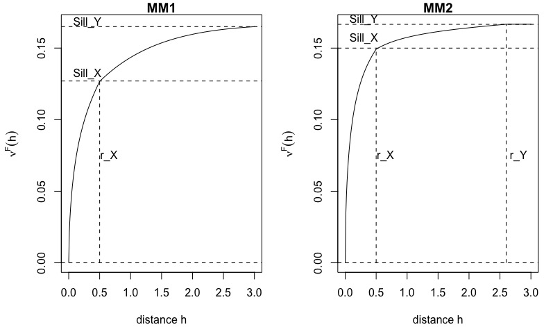
Figure 1. $h\leadsto\nu^{F}(h)$ for the max-mixture processes models MM1 and MM2. In MM1, $X$ has correlation function $\rho(h)=\exp(-h/\theta_{X})$, $r_{X}=0.25$ and fixed radius $\theta_{X}=0.2$ and $Y$ has $\Sigma=\sigma_{Y}\bf I_{d}$, $\sigma_{Y}=0.6$. In MM2, $X$ has the same setting as in MM1 and $Y$ has $\rho_{Y}(h)=\exp(-h/\theta_{Y})$, $\theta_{Y}=0.8$ and fixed radius $r_{Y}=1.35$. For the two models, we set $a=0.5$.

4. Model inference

This section is devoted to the parametric inference for max-mixture processes. We begin with the presentation of the maximum composite likelihood estimation, then we present the least squares madogram estimation.

4.1. Parametric Estimation using Composite Likelihood

Consider $(Z^{k}(s_{1})\/,\ldots\/,Z^{k}(s_{D}))$, $k=1\/,\ldots\/,N$, be $N$ independent copies of a spatial process $(Z(s))_{s\in\mathbb{S}}$, observed at $D$ locations $s_{1}\/,\ldots\/,s_{D}$. Composite likelihood inference is an appropriate approach in estimating the parameter models of a spatial process $X$ ([lindsay1888composite, varin2011overview]). Asymptotic properties of this estimator has been proved in [davis2011comments]. This approach has been applied successfully to spatial max-stable processes by [davison2012geostatistics] and [padoan2010likelihood] and is also used to identify the parameters of data exceedances over a large threshold, for example, [bacro2014estimation] and [thibaud2013threshold]. In this article, we focus on max-mixture models. Composite likelihood inference for max-mixture processes has been studied in [bacro2016flexible] and [wadsworth2012dependence]. We will compare our madogram based estimation to the composite likelihood estimation described in [bacro2016flexible].

If the pairwise density of $Z$ can be computed and its parameter $\psi$ is identifiable, then it is possible to estimate $\psi$ by maximizing the pairwise weighted log likelihood. For simplicity, we denote $Z_{i}^{k}$ for $Z^{k}(s_{i})$. Let

$$\widehat{\psi}_{L}=\max_{\psi}\mathcal{P}(\psi),$$

where

(4.1) $$\mathcal{P}(\psi)=\sum_{k=1}^{N}\sum_{i=1}^{D-1}\sum_{j>i}^{D}w_{ij}\log\mathscr{L}(Z_{i}^{k},Z_{j}^{k};\psi)=:\sum_{k=1}^{N}\mathcal{P}_{k}(\psi)\/.$$

where $\mathscr{L}$ is the likelihood of the pair $(Z_{i}^{k},Z_{j}^{k})$ and $w_{i,j}\geq 0$ is the weight that specifies the contribution for each pair. In [padoan2010likelihood], it is suggested to
In [coles2001introduction], it is suggested to consider a censor approach of the likelihood, taking into account a threshold. This approach has been adopted in this study. Let $G(\cdot,\cdot)$ be a pairwise distribution function and consider the thresholds $u_{1}$ and $u_{2}$; the likelihood contribution is

$$\mathscr{L}(z_{1},z_{2};\psi)=\begin{cases}\partial^{2}_{12}G(z_{1},z_{2};\psi)&\mbox{if}\ z_{1}>u_{1},z_{2}>u_{2},\\ G(z_{1},z_{2};\psi)&\mbox{if}\ z_{1}\leq u_{1},z_{2}\leq u_{2},\end{cases}$$

In [wadsworth2012dependence], the censored likelihood is used in order to improve the estimation of the parameters related to asymptotic independence. This censored approach was also applied by [bacro2016flexible] for the estimation of parameters of max-mixture processes. In that paper, the replications $Z^{1}\/,\ldots\/,Z^{N}$ of $Z$ are assumed to be $\alpha$-mixing rather than independent. We denote generically by $\psi$ the parameters of the model. In [bacro2016flexible], it is proved, under some smoothness assumptions on the composite likelihood, that the composite maximum likelihood estimator $\widehat{\psi}_{L}$ for max-mixture processes is asymptotically normal as $N$ goes to infinity with asymptotic variance

$$\mathscr{G}(\psi)=\mathcal{J}(\psi)[\mathcal{K}(\psi)]^{-1}\mathcal{J}(\psi),$$

where $\mathcal{J}(\psi)=\mathbb{E}[-\nabla^{2}\mathcal{P}(\psi)]$, $\mathcal{K}(\psi)=\mathrm{var}(\nabla\mathcal{P}(\psi))$. The matrix $\mathscr{G}(\psi)$ is called the Godambe information matrix (see [bacro2016flexible] and Theorem 3.4.7 in [guyon1995random]).
An estimator $\widehat{\mathcal{J}}$ of $\mathcal{J}(\psi)$ is obtained from the Hessian matrix computed in the optimization algorithm. The variability matrix ${\mathcal{K}}(\psi)$ has to be estimated too. In our context, we have independent replications of $Z$ and $N$ is large compared with respect to the dimension of $\psi$. Then, we can use the outer product of the estimation of $\widehat{\psi}$. Let

$$\widehat{\mathcal{K}}(\psi)=N^{-1}\sum_{k=1}^{N}\nabla\mathcal{P}_{k}(\widehat{\psi})\nabla\mathcal{P}_{k}(\widehat{\psi})^{\prime}$$

or by Monte Carlo simulation with explicit formula of $\mathcal{P}_{k}(\psi)$ (see section 5. in [varin2011overview]). In the case of samples of $Z$ satisfying the $\alpha$-mixing property, the estimation of $\mathcal{K}(\psi)$ can be done using a subsampling technique introduced by [carlstein1986use]; this was used in [bacro2016flexible]. Finally, model selection can be done by using the composite likelihood information criterion [varin2005note]:

$$\mathrm{CLIC}=-2\bigg{[}\mathcal{P}(\widehat{\psi})-tr(\widehat{\mathcal{J}}^{-1}\widehat{\mathcal{K}})\bigg{]}.$$

Considering several max-stable models, the one that has the smallest CLIC will be chosen. In [thibaud2013threshold], the criterion $\mathrm{CLIC}^{*}=(D-1)^{-1}\mathrm{CLIC}$ is proposed. It is close to Akaike information criterion (AIC).

4.2. Semi-parametric estimation using NLS of F-madogram

In this section, we shall define the non-linear least square estimation procedure of the parameters set $\psi$ corresponding to the max-mixture model $Z$ using the $F$-madogram. This procedure can be considered as an alternative method to the composite likelihood method.
Consider $Z^{k}$, $k=1\/,\ldots\/,N$ copies of an isotropic max-mixture process $Z$ with unit Fréchet marginal laws ($F$ denotes the distribution function of a unit Fréchet law). It may be independent copies for example, if the data is recorded yearly (see [naveau2009modelling]) or we shall consider that $(Z^{k})_{k=1\/,\ldots\/,N}$ satisfies a $\alpha$-mixing property ([bacro2016flexible]). Let $\mathcal{H}$ be a finite subset of $\mathbb{S}$, $J(x,y)=\frac{1}{2}|x-y|$ and $Y_{h,k}=J\big{(}F(Z^{k}(s)),F(Z^{k}(s+h))\big{)}$, $k=1,..,N$ and $h\in\mathcal{H}$. Therefore, for $k=1\/,\ldots\/,N$, the vectors $(Y_{h\/,k})_{h\in\mathcal{H}}$ have the same law and are considered either independent or $\alpha$-mixing (in $k$). The main motivation for using the F-madogram in estimation is that it contains the dependence structure information for a fixed $h$ of $Y_{h,k}$ (see Section 3.2 in [bacro2010testing]).
In what follows, we make the assumption that the vectors $(Y_{h\/,k})_{h\in\mathcal{H}}$ are i.i.d. Note that from the definition of the $F$-madogram, we have $\mathbb{E}[Y_{h,k}]=\nu^{F}(h,\psi)$ where $\nu^{F}(h,\psi)$ is the $F$-madogram of $Z$ with parameters $\psi$ defined in (3.1). If $Z$ has an unknown true parameter $\psi_{0}$ on a compact set $\Psi\subset\mathbb{R}^{d}$, we rewrite

(4.2) $$Y_{h,k}=\nu^{F}(h,\psi_{0})+\varepsilon_{h,k}.$$

The vectors $(\varepsilon_{h,k})_{h\in\mathcal{H}}$ are i.i.d errors with $\mathbb{E}[\varepsilon_{h,k}]=0$ and $\mbox{Var}(\varepsilon_{h,k})=\sigma_{h}^{2}>0$ is finite and unknown.
Let

(4.3) $$\mathcal{L}(\psi)=\sum_{h\in\mathcal{H}}\frac{1}{N}\sum_{k=1,...,N}\big{(}Y_{h,k}-\nu^{F}(h,\psi)\big{)}^{2}$$

Any vector $\widehat{\psi}_{M}$ in $\Psi$ which minimizes $\mathcal{L}(\psi)$ will be called a least square estimate of $\psi_{0}$:

(4.4) $$\widehat{\psi}_{M}\in\operatorname*{argmin}_{\psi\in\Psi}\mathcal{L}(\psi)\/.$$

Theorem 4.1.

Assume that $\Psi\subset\mathbb{R}^{d}$ is compact and that $\psi\mapsto\nu^{F}(h\/,\psi)$ is continuous for all $h\in\mathcal{H}$. We assume that the vectors $(Y_{h\/,k})_{h\in\mathcal{H}}$ are i.i.d. Let $(\widehat{\psi}_{M}^{N})_{N\in\mathbb{N}}$ be least square estimators of $\psi_{0}$. Then, any limit point (as $N$ goes to infinity) $\psi$ of $(\widehat{\psi}_{M}^{N})_{N\in\mathbb{N}}$ satisfies $\nu(h\/,\psi)=\nu(h\/,\psi_{0})$ for all $h\in\mathcal{H}$.

Remark 4.1.

Of course, if $\psi\leadsto(\nu(h\/,\psi))_{h\in\mathcal{H}}$ is injective, then Theorem 4.1 implies that the least square estimation is consistent, i.e. $\widehat{\psi}_{M}^{N}\rightarrow\psi_{0}$ a.s. as $T$ goes to infinity. In the examples considered below, it seems that the injectivity is satisfied provided $|\mathcal{H}|\geq d$, but we were unable to prove it.

Proof.

We follow the proof of Theorem II.5.1 in [antoniadis1992regression]. From (4.2), we have, for all $\psi\in\Psi$

$$\begin{split}\mathcal{L}(\psi)=&\sum_{h\in\mathcal{H}}\frac{1}{N}\sum_{k=1,...,N}\big{(}\nu^{F}(h,\psi_{0})+\varepsilon_{h,k}-\nu^{F}(h,\psi)\big{)}^{2}\\ =&\sum_{h\in\mathcal{H}}\big{(}\nu^{F}(h,\psi_{0})-\nu^{F}(h,\psi)\big{)}^{2}\\ +&\frac{2}{N}\sum_{h\in\mathcal{H}}\big{(}\nu^{F}(h,\psi_{0})-\nu^{F}(h,\psi)\big{)}\left(\sum_{k=1,...,N}\varepsilon_{h,k}\right)+\sum_{h\in\mathcal{H}}\frac{1}{N}\sum_{k=1,...,N}\varepsilon_{h,k}^{2}.\end{split}$$

From the law of large numbers, we have

$$\frac{1}{N}\sum_{h\in\mathcal{H}}\sum_{k=1,...,N}\varepsilon_{h,k}^{2}\to\sum_{h\in\mathcal{H}}\sigma_{h}^{2}\quad\mathrm{a.s.}\quad\mathrm{as}\quad N\to\infty$$

and for any $h\in\mathcal{H}$,

$$\frac{1}{N}\sum_{k=1,...,N}\varepsilon_{h,k}\to 0\ \mbox{a.s.}$$

Therefore,

$$\mathcal{L}(\psi)\to\sum_{h\in\mathcal{H}}\sigma_{h}^{2}+\sum_{h\in\mathcal{H}}\big{(}\nu^{F}(h,\psi_{0})-\nu^{F}(h,\psi)\big{)}^{2}\quad\mathrm{a.s.}\quad\mathrm{as}\quad N\to\infty.$$

Take a sequence $(\widehat{\psi}_{M}^{N})_{N\in\mathbb{N}}$ of least square estimators, taking if necessary a subsequence, we may assume that it converges to some $\psi^{*}\in\Psi$. Using the continuity of $\psi\leadsto\nu^{F}(h\/,\psi)$, we have

$$\mathcal{L}(\widehat{\psi}_{M}^{N})\rightarrow\sum_{h\in\mathcal{H}}\sigma_{h}^{2}+\sum_{h\in\mathcal{H}}\big{(}\nu^{F}(h,\psi_{0})-\nu^{F}(h,\psi^{*})\big{)}^{2}\quad\mathrm{a.s.}\quad\mathrm{as}\quad N\to\infty.$$

Since $\widehat{\psi}_{M}^{N}$ is a least square estimator, $\mathcal{L}(\widehat{\psi}_{M}^{N})\leq\mathcal{L}(\psi_{0})\rightarrow\displaystyle\sum_{h\in\mathcal{H}}\sigma_{h}^{2}$. It follows that

$$\sum_{h\in\mathcal{H}}\big{(}\nu^{F}(h,\psi_{0})-\nu^{F}(h,\psi^{*})\big{)}^{2}=0$$

and thus $\nu(h\/,\psi^{*})=\nu(h\/,\psi_{0})$ for all $h\in\mathcal{H}$. ∎

The asymptotic normality of the least square estimators should also be obtained by following, e.g., [buhl2016Semiparametric] and using the asymptotic normality of the $F$-madogram obtained in [cooley2006variograms]. Nevertheless, the calculation of the asymptotic variance will require to calculate the covariances between $\nu^{F}(h_{1}\/,\psi)$ and $\nu^{F}(h_{2}\/,\psi)$, which is not straightforward.

5. Simulation study

This section is devoted to some simulations in order to evaluate the performance of the least square estimator and to compare it with the maximum composite likelihood estimator. Recall that $\widehat{\psi}_{M}$ denotes the least square estimator of the parameter vector $\psi$ and $\widehat{\psi}_{L}$ denotes the composite likelihood estimator.

5.1. Outline the simulation experiment

In order to evaluate the performance of the non-linear least square estimator $\widehat{\psi}_{M}$ as defined in (3.1), we have generated data from the model MM1 above. The least square madogram estimator $\widehat{\psi}_{M}$ has been compared with true one $\psi_{0}$ and also with parameters estimated by maximum composite likelihood $\widehat{\psi}_{L}$ proposed in [bacro2016flexible, wadsworth2012dependence], on the same simulated data. We considered $50$ sites randomly and uniformly distributed in the square ${\mathcal{A}}=[0,1]^{2}$.
We have generated $N=1.000$ i.i.d observations for each site and replicated this experiment $J=100$ times. We have considered several mixing parameters: $a:=\{0,0.25,0.5,0.75,1\}$. For the composite likelihood estimator $\widehat{\psi}_{L}$, we used the censored procedure with the $0.9$ empirical quantile of data at each site as threshold $u$. The fitting of $\widehat{\psi}_{L}$ was done using the code which was used in [bacro2016flexible] with some appropriated modifications.

5.2. Results on the parameters estimate

In Figure 3, we represented the boxplots of the errors, that is $(\widehat{\psi}_{M}-\psi_{0})$ and $(\widehat{\psi}_{L}-\psi_{0})$ for model MM1. Generally, the estimators above worked well, although the variability in some estimates were relatively large, especially for the asymptotic independence parameters. It also shows some bias in the estimation of the asymptotic independence model parameters.

It is well known that asymptotic independence is difficult to estimate (see [davison2013geostatistics]). Therefore, the estimation accuracy of the parameters is very sensitive. On one other hand, the fitting of $\alpha(h)$ which appears in TEG models in (2.17), is delicate and might lead to quite different estimates with different data [davison2012geostatistics].

 

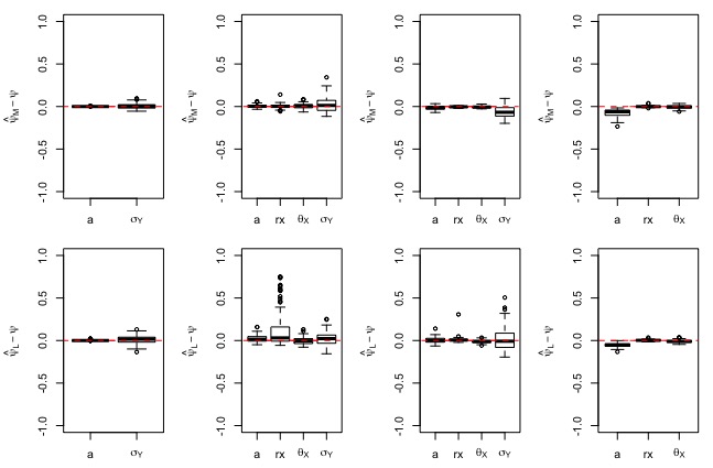
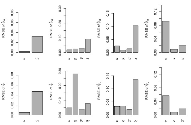
Figure 2. Boxplots display $(\widehat{\psi}-\psi)$ of estimated parameters vector $\widehat{\psi}=(\widehat{a},\widehat{r}_{X},\widehat{\theta}_{X},\widehat{\sigma}_{Y})^{T}$ for the MM1 model by the two estimators $\widehat{\psi}_{M}$ and $\widehat{\psi}_{L}$. The figures in the first row and from left to right concern the estimator $\widehat{\psi}_{M}$ for $a\in\{0,{\color[rgb]{0,0,0}0.25},0.75,1\}$, the second row concerns $\widehat{\psi}_{L}$. We have set, $r_{X}=0.25$, $\theta_{X}=0.20$ and $\sigma_{Y}=0.6$ over a square ${\mathcal{A}}=[0,1]^{2}$.

Figure 3. Barplots display the RMSE of $\widehat{\psi}$ for each estimated parameters $\widehat{\psi}=(\widehat{a},\widehat{r}_{X},\widehat{\theta}_{X},\widehat{\sigma}_{Y})^{T}$ for MM1 and the corresponding two estimators $\widehat{\psi}_{M}$ and $\widehat{\psi}_{L}$. The bars in the first row and from left to right represent the RMSE of the estimator $\widehat{\psi}_{M}$ when $a:=\{0,{\color[rgb]{0,0,0}0.25},0.75,1\}$, respectively and the same for the second row for $\widehat{\psi}_{L}$. We set $r_{X}=0.25$, $\theta_{X}=0.20$ and $\sigma_{Y}=0.6$ over a square ${\mathcal{A}}=[0,1]^{2}$.

Another comparison indicator is the root mean square error (RMSE) ([zheng2015assessing, zheng2014modeling]): let $\widehat{\psi_{j}}$ denote the $j$th estimation (either least square or composite likelihood estimation),

(5.1) $$\mathrm{RMSE}=\bigg{[}J^{-1}\sum_{j=1}^{J}(\widehat{\psi_{j}}-\psi)^{2}\bigg{]}^{1/2},$$

The barplot in Figure 3 displays the RMSE for each parameter of MM1 model. We see on these barplots that when $a$ is close to $0$ ($a=0;0.25$), the estimator $\widehat{\psi}_{M}$ over-performs the estimator $\widehat{\psi}_{L}$ and vice versa when $a\in\{0.75,1\}$. For $a=0.5$ the performance of the two estimators seem equivalent.

5.3. Asymptotic normality

We may figure out whether the least square estimator $\widehat{\psi}_{M}$ is asymptotically normal through the graphe of the errors $\widehat{\psi}_{L}-\psi_{0}$. In Figure 4, the graphs represent the distributions of the errors of each estimated parameters of MM1 model for $a:=\{0,0.5,1\}$. We did $J=500$ simulation experiments.
We can see on Figure 4 that the densities of the errors of the parameters seem close to the shape of centered normal distribution.

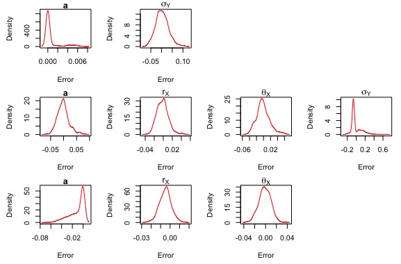
Figure 4. Graphs display the densities of the errors between $\widehat{\psi}_{M}$ and $\psi_{0}$ for each estimated parameters in the set $\psi=(a,r_{X},\theta_{X},\sigma_{Y})^{T}$ of MM1 model. The graphs from first row and last one represent the densities of the errors $\widehat{\psi}_{M}-\psi_{0}$ when $a:=\{0,0.5,1\}$. We set $r_{X}=0.25$, $\theta_{X}=0.20$ and $\sigma_{Y}=0.6$ over a square ${\mathcal{A}}=[0,1]^{2}$.

6. Real data example

In this section, we analyze a real data and fit it to some models considered in this study by composite likelihood and LS-madogram procedures.

6.1. Data analysis

We analyzed daily rainfall along the east coast of Australia. We selected 39 locations randomly from this region. The data is daily measured in the period from April to September for 35 years from 1982-2016. The data is available from the Australian Bureau of Meteorology (http://www.bom.gov.au/climate/data/).

In order to explore the possibility of anisotropy of the spatial dependence, we used the same test as in [bacro2016flexible]. We divided all data set according to directional sectors $(-\pi/8,\pi/8]$, $(\pi/8,3\pi/8]$, $(3\pi/8,5\pi/8]$ and $(5\pi/8,7\pi/8]$, where $0$ indicate to north direction. We use the empirical F-madogram $\widehat{\nu}^{F}(h)$. The directional loss smoothing of such empirical measure in the Figure 5. (A), shows no evidence of anisotropy.

In Figure 5. (B), the empirical F-madogram is plotted for the whose data set. It seems that asymptotic dependence between the locations is present up to distance 500 km and asymptotic independence could be present at the remaining distance.

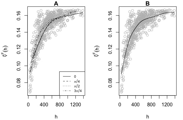
Figure 5. Empirical evaluation of $\widehat{\nu}^{F}(h)$. The Grey circles represented the empirical value between all pairs. The lines in (A) represent the smoothed value of the empirical of $\widehat{\nu}^{F}(h)$ according to directional sectors $(-\pi/8,\pi/8]$, $(\pi/8,3\pi/8]$, $(3\pi/8,5\pi/8]$ and $(5\pi/8,7\pi/8]$. The line in (B) represent the smoothed value of the empirical of $\widehat{\nu}^{F}(h)$ for all directions.

6.2. Data fitting

Our interest in this section is to chose a reasonable model for the data. We considered $7$ models described below, for each model, the parameters are estimated by LS-madogram and maximum composite likelihood. The selection criteria for LS-madogram estimator $\widehat{\psi}_{M}$ is computed as the following:

$$MIC:=\log{\mathcal{L}(\widehat{\psi})}+(2k(k+1)/(T-k-1)),$$

where $k$ is the number of parameters in the model and $T$ is the number of the observations, that is: $T=N\times|\mathcal{H}|$, where $|\mathcal{H}|$ is the number of observed pairs. With respect to censored composite likelihood estimators we adopted the CLIC selection criteria. The two criteria selected the model MM1 as the best model.
We consider the following models:

MM1:

max-mixture between asymptotic dependence process represented by TEG max-stable process $X$ with exponential correlation function $\rho(h)=\exp\{-(h/\theta_{X})\},\theta_{x}>0$ and $\mathcal{B}_{X}$ is a disk of fixed and unknown radius $r_{X}$. The asymptotic independence is represented by an inverse Brown-Resnik max-stable process $Y$ with variogram $2\gamma(h)=2\sigma^{2}{(1-\exp\{-(h/\theta_{Y})\})}$, $\theta_{Y},\sigma>0$; $\sigma^{2}$ is the sill of the variogram.

MM2:

max-mixture between $X$ as in MM1 and an inverse inverse Smith max-stable process $Y$ with $\tau(h)=h/\sqrt{\sigma_{Y}}$.

M1:

A TEG max-stable process $X$ specified in MM1.

M2:

A Brown-Resnik max-stable process $X$ as specified in MM1.

M3:

An inverse Brown-Resnik max-stable process $Y$ as specified in MM1.

M4:

A Smith max-stable process $X$ as specified in M2.

M5:

A inverse Smith max-stable process $Y$ as specified in M2.

For all the considered models, the margin distribution are assumed to be unit Fréchet. Therefore it requires to transform the data set to Fréchet. Most of papers (see for example [bacro2016flexible] and [wadsworth2012dependence]) use parametric transformations: they fit GEV parameters for each location separately and then transform the data to Fréchet. In this study, we adopted a non-parametric transformation by using the empirical c.d.f.. For censored composite likelihood procedures, we set $u=0.9$ and $\delta=\infty$.

Table 1. Summary of the fitted models. the distance scale is kilometres. Composite likelihood procedure indicated by CL and LS-madogram procedure indicated by LS with selection criteria SC are CLIC and MIC, respectively.

Model		a	$\theta_{X}$	$r_{X}$	$\theta_{Y}$	$\sigma_{Y}$	SC
MM1	CL	0.262	1217.3	1364.5	3102.4	3.457	6807406
	LS	0.259	1285.7	1390.0	5794.8	2.013	1.917034
MM2	CL	0.248	31.16	70.15	998.84		7924609
	LS	0.185	35.51	48.14	871.19		1.917234
		$\theta_{X}$	$r_{X}$
M1	CL	931	307.86				7926261
	LS	1270	255.64				1.945177
		$\theta_{X}$	$\sigma_{X}$	$\theta_{Y}$	$\sigma_{Y}$
M2	CL	931.02	3.078663				7926261
	LS	361.36	1.90816				1.96165
M3	CL			1644.76	2.702282		7918643
	LS			1383.08	1.394928		1.924574
M4	CL		85.34				8016633
	LS		193.43				1.988753
M5	CL					256.39	7988838
	LS					334.60	1.929235

We remark that the two Decision Criteria (CLIC and MIC) choose the same model. We would like to emphasize that CLIC and MIC are not comparable, one is related to the composite likelihood while the other one is related to the least squared madogram difference. For the tested models, we would keep the model with the smallest CLIC or the smallest MIC, depending on the used estimation method. Also, the least squared madogram estimation is involves less computations, indeed, the maximum composite likelihood estimation requires to estimate the Godambe matrix in order to compute the CLIC.

7. Conclusions

The calculation of the F-madogram for max-mixture processes show that it writes with both the AD and the AI parameters. This leads us to propose a semi-parametric estimation procedure using F-madogram ${\nu}^{F}(h)$ as an alternative to composite likelihood. The simulation study showed that the estimation procedure based on $\nu^{F}(h)$ performs better than the composite likelihood procedure when the model is near to asymptotic independence. We applied these estimator procedures to real data example. On the considered example, the results obtained by composite likelihood maximization and least squared madogram difference are similar.
 
Acknowledgements: This work was supported by the LABEX MILYON (ANR-10-LABX-0070) of Université de Lyon, within the program “Investissements d’Avenir” (ANR-11-IDEX-0007) operated by the French National Research Agency (ANR). We also acknowledge the projet LEFE CERISE.