Verifications of primal energy identities for variational problems with obstacles

Abstract

We discuss error identities for two classes of free boundary problems generated by obstacles. The identities suggest true forms of the respective error measures which consist of two parts: standard energy norm and a certain nonlinear measure. The latter measure controls (in a weak sense) approximation of free boundaries. Numerical tests confirm sharpness of error identities and show that in different examples one or another part of the error measure may be dominant.

1 Introduction

New types of error identities were recently derived [8] for two types of inequalities generated by obstacle type conditions: a classical obstacle problem and a two-phase obstacle problem. Both problems belong to the class of variational problems

$$\inf\limits_{v\in V}J(v),\qquad J(v)=G(\Lambda v)+F(v),$$ (1)

where $\Lambda:V\rightarrow Y$ is a bounded linear operator, $G:Y\rightarrow{\mathbb{R}}$ is a convex, coercive, and lower semicontinuous functional, $F:V\rightarrow{\mathbb{R}}$ is another convex lower semicontinuous functional, and $Y$ and $V$ are reflexive Banach spaces. Henceforth, we use results of [6] related to derivation of a posteriori error estimates for this class of problems.

1.1 The classical obstacle problem

The classical obstacle problem (see, e.g. [2, 3]) is characterized by

$$G(\Lambda v)=\frac{1}{2}\int\limits_{\Omega}A\nabla v\cdot\nabla v\,dx,\qquad F(v)=-\int\limits_{\Omega}fv\,dx+\chi_{K}(v),$$

where the characteristic functional is defined as

$$\chi_{K}(v):=\left\{\begin{array}[]{cc}0&{\rm if}\;\phi\leq v\leq\psi,\\ +\infty&{\rm else}\end{array}\right.$$

and the admissible set reads

$$K:=\{v\in V_{0}:=H^{1}_{0}(\Omega)\,\mid\,\phi(x)\,\leq v(x)\,\leq\psi(x)\;{\rm a.e.\,in\,}\Omega\}.$$

Here, $H^{1}_{0}(\Omega)$ denotes the Sobolev space of functions vanishing on $\partial\Omega$ (hence we consider the case $u_{D}=0$), $\Omega\subset\mathbb{R}^{d}$ ($d\in\{1,2,3\}$) is a bounded domain with a Lipschitz continuous boundary $\partial\Omega$ and $\phi,\psi\in H^{2}(\Omega)$ are two given functions (lower and upper obstacles) such that

$$\phi(x)\leq 0\;{\rm on}\;\partial\Omega,\quad\psi(x)\geq 0\;{\rm on}\;\partial\Omega,\quad\phi(x)\leq\psi(x),\quad\forall x\in\Omega.$$

It is assumed that $A$ is a symmetric matrix subject to the condition

$$A(x)\xi\cdot\xi\geq c_{1}\,|\xi|^{2}\qquad c_{1}>0,\qquad\forall\xi\in\mathbb{R}^{d}$$ (3)

almost everywhere in $\Omega$. Under the assumptions made, the unique solution $u\in K$ exists. The mechanical motivation of the obstacle problem is to find the equilibrium position of an elastic membrane whose boundary is held fixed, and which is constrained to lie between given lower and upper obstacles $\phi$ and $\psi$.

1.2 The two-phase obstacle problem

The functional $J(v)$ of the two-phase-obstacle problem (see, e.g. [9]) is defined by the relation

$$J(v):=\int\limits_{\Omega}\Big{(}\frac{1}{2}A\nabla v\cdot\nabla v-fv+\alpha_{+}(v)_{+}+\alpha_{-}(v)_{-}\Big{)}\,dx.$$ (4)

The functional $J(v)$ is minimized on the set

$$V_{0}+u_{D}:=\{v=v_{0}+u_{D}\,:\,v_{0}\in V_{0},\;u_{D}\in H^{1}(\Omega)\}.$$

Here $u_{D}$ is a given bounded function that defines the boundary condition ($u_{D}$ may attain both positive and negative values on different parts of the boundary $\partial\Omega$). It is assumed that the coefficients $\alpha_{+},\alpha_{-}:\Omega\rightarrow\mathbb{R}$ are positive constants (without essential difficulties the consideration and main results can be extended to the case where they are positive Lipschitz continuous functions). Also, it is assumed that $f\in L^{\infty}(\Omega)$, $A\in L^{\infty}(\Omega,\mathbb{R}^{d\times d})$, and the condition (3) holds. Since the functional $J(v)$ is strictly convex and continuous on $V$, existence and uniqueness of a minimizer $u\in V_{0}+u_{D}$ is guaranteed by well known results of the calculus of variations. The mechanical motivation of the two-phase obstacle problem is to find the equilibrium position of an elastic membrane in the two-phase matter with different gravitation densities related to $\alpha_{-}$ and $\alpha_{+}$.

2 Error identities

The solution $u$ of the classical obstacle problem divides $\Omega$ into three sets:

$$\Omega^{u}_{-}:= \{x\in\Omega\,\mid\,u(x)=\phi(x)\}\,,$$

$$\Omega^{u}_{+}:= \{x\in\Omega\,\mid\,u(x)=\psi(x)\}\,,$$

$$\Omega^{u}_{0}:= \{x\in\Omega\,\mid\,\phi(x)<u(x)<\psi(x)\}\,.$$

The sets $\Omega^{u}_{-}$ and $\Omega^{u}_{+}$ are the lower and upper coincidence sets and $\Omega^{u}_{0}$ is an open set, where $u$ satisfies the Poisson equation ${\rm div}(A\nabla u)+f=0$. Thus, the problem involves free boundaries, which are unknown a priori. Let $v$ be an approximation of $u$. It defines approximate sets

$$\Omega^{v}_{-}:= \{x\in\Omega\,\mid\,v(x)=\phi(x)\}\,,$$

$$\Omega^{v}_{+}:= \{x\in\Omega\,\mid\,v(x)=\psi(x)\}\,,$$

$$\Omega^{v}_{0}:= \{x\in\Omega\,\mid\,\phi(x)<v(x)<\psi(x)\}\,.$$

Notice that unlike the sets in (2), the sets (2) are known.

Theorem 2.1 ([8])

Let $v\in K$ be any approximation of the exact solution $u\in K$ of the classical obstacle problem. Then it holds

$$\frac{1}{2}||\nabla(u-v)||_{A}^{2}+\mu_{\phi\psi}(v)=J(v)-J(u),$$ (7)

where

$$\mu_{\phi\psi}(v):=\!\int\limits_{\Omega^{u}_{-}}\!\!{\sf W}_{\phi}(v-\phi)\,dx+\int\limits_{\Omega^{u}_{+}}\!\!{\sf W}_{\psi}(\psi-v)\,dx,$$ (8)

and ${\sf W}_{\phi}:=-({\rm div}A\nabla\phi+f),{\sf W}_{\psi}:={\rm div}A\nabla\psi+f$ are two nonnegative weight functions generated by the source term $f$, the obstacles $\psi,\phi$ and the diffusion $A$.

Here, $\mu_{\phi\psi}(v)$ represents a certain (non-negative) measure, which controls (in a weak integral sense) whether or not the function $v$ coincides with obstacles $\psi,\phi$ on true coincidence sets $\Omega^{u}_{-}$ and $\Omega^{u}_{+}$.

Remark 1

The error identity (7) was derived for the homogeneous boundary condition $u=0$ on $\partial\Omega$, but it is possible to extend it in the same form to for the nonhomogeneous boundary condition $u\not=0$ on $\partial\Omega$.

For the two-phase obstacle problem, we introduce two decompositions (diffent from the classical obstacle problem) of $\Omega$ associated with the minimizer $u$ and an approximation $v$:

$$\Omega^{u}_{-}:=\{x\in\Omega\,\mid\,u(x)<0\},$$

$$\Omega^{u}_{+}:=\{x\in\Omega\,\mid\,u(x)>0\},$$ (9)

$$\Omega^{u}_{0}:=\{x\in\Omega\,\mid\,u(x)=0\},$$

and

$$\Omega^{v}_{-}:=\{x\in\Omega\,\mid\,v(x)<0\},$$

$$\Omega^{v}_{+}:=\{x\in\Omega\,\mid\,v(x)>0\},\$$ (10)

$$\Omega^{v}_{0}:=\{x\in\Omega\,\mid\,v(x)=0\}.$$

These decompositions generate exact and approximate free boundaries. If we introduce new sets

$$\omega_{+}:=\Omega^{v}_{+}\cap\Omega^{u}_{0},\quad\omega_{-}:=\Omega^{v}_{-}\cap\Omega^{u}_{0},\quad\omega_{\pm}:=\left\{\Omega^{v}_{+}\cap\Omega^{u}_{-}\right\}\cup\left\{\Omega^{v}_{-}\cap\Omega^{u}_{+}\right\},$$

we can formulate an error identity for the two-phase obstacle problem.

Theorem 2.2 ([7],[8])

Let $v\in V_{0}+u_{D}$ be any approximation of the exact solution $u\in V_{0}+u_{D}$ of the two-phase obstacle problem. Then it holds

$$\frac{1}{2}||\nabla(u-v)||_{A}^{2}+\mu_{\omega}(v)=J(v)-J(u),$$ (11)

where

$$\mu_{\omega}(v):=\int\limits_{\omega}\alpha(x)|v|\,dx,\quad\omega:=\omega_{+}\cup\omega_{-}\cup\omega_{\pm}$$ (12)

and

$$\alpha(x):=\left\{\begin{array}[]{ll}\alpha(x)=\alpha_{+}&{\rm if}\;x\in\,\omega_{+},\\ \alpha(x)=\alpha_{-}&{\rm if}\;x\in\,\omega_{-},\\ \alpha(x)=\alpha_{+}+\alpha_{-}&{\rm if}\;x\in\,\omega_{\pm}.\end{array}\right.$$ (16)

Here, $\mu_{\omega}(v)$ represents another nonlinear measure (which differs from $\mu_{\phi\psi}$).

3 Numerical verifications

We verify a posteriori error identities (7) and (11) for both obstacle problems and focus on interpretation of their nonlinear measures $\mu_{\phi\psi}(\cdot)$ and $\mu_{\omega}(\cdot)$. Another goal is to present examples with different balance between two components of the overall error measure.

3.1 The classical obstacle problem in 2D

We assume a 2D example taken from [5]. In this example, $\Omega=(-1,1)^{2},A=\mathbb{I},\phi=0,\psi=+\infty$ It is known that for

$$f(x,y)=\left\{\begin{array}[]{lrl}-16(x^{2}+y^{2})+8R^{2}&\quad\textrm{if}&\sqrt{x^{2}+y^{2}}>R\\ -8(R^{4}+R^{2})+8R^{2}(x^{2}+y^{2})&\quad\textrm{if}&\sqrt{x^{2}+y^{2}}\leq R\end{array}\right.,$$

where $R\in[0,1)$ is given, the exact solution to the obstacle problem reads

$$u(x,y)=\left\{\begin{array}[]{lrll}\left(\max\{x^{2}+y^{2}-R^{2},0\}\right)^{2}&\quad\mbox{if}&(x,y)\in\Omega\\ \left(x^{2}+y^{2}-R^{2}\right)^{2}&\quad\mbox{if}&(x,y)\in\partial\Omega\end{array}\right..$$

The corresponding energy can be computed (see [4]) and it reads

$$J(u)=192\left(\frac{12}{35}-\frac{28R^{2}}{45}+\frac{R^{4}}{3}\right)-32R^{2}\left(\frac{28}{45}-\frac{4R^{2}}{3}+R^{4}\right)+\frac{2}{3}\pi R^{8}.$$

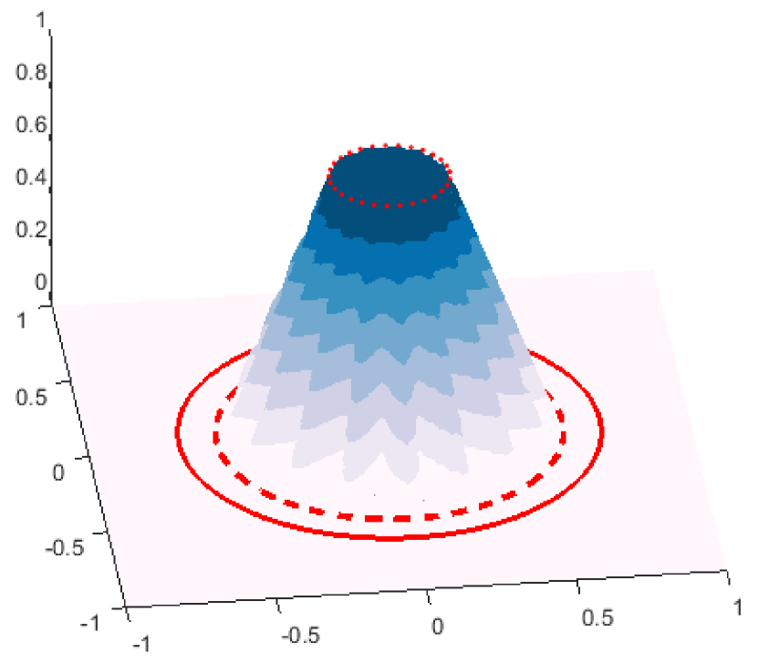
Figure 1: A perturbation function $w$ (left) generated by parameters $R=0.7,r=0.2,k=16$ and the same corresponding coincidence set $\Omega^{v}_{-}$ (right) for all approximative solutions $v=u+\epsilon\,w$, where $\epsilon>0$. The boundary of $\Omega^{u}_{-}$ is indicated by the full circle, the inner radius $r$ by the dotted circle and the intermediate radius $\frac{r+3R}{4}$ by the dashed circle.

We consider approximations $v$ in the form

$$v_{\epsilon}:=u+\epsilon\,w,$$ (17)

where $\epsilon>0$ is a given amplitude and $w$ is a solution perturbation defined in polar coordinates $(\rho,\theta)$ as

$$w(\rho,\theta):=\left\{\begin{array}[]{ll}1,&\text{if }\rho\leq r\\ 1-\frac{\rho-r}{\tilde{r}(\theta)-r},&\text{if }r\leq\rho\leq\tilde{r}(\theta)\\ 0,&\text{if }\rho\geq\tilde{r}(\theta)\end{array}\right..$$ (18)

Here, $0<r<R$ is given internal radius and a variable radius $\tilde{r}(\theta)$ is defined as

$$\tilde{r}(\theta):=r+(R-r)\left(\frac{2+\cos(k\theta)}{4}\right)$$ (19)

for some $k\in\mathbb{Z}$. This construction ensures that

$$r<\frac{3r+R}{4}\leq\tilde{r}(\theta)\leq\frac{r+3R}{4}<R$$ (20)

and consequently $\nabla w$ is bounded. An examples of perturbations $w$ is visualized in Figure 1 together with corresponding coincidence sets $\Omega^{v}_{-}$. For given $k$ and $r$, there is always a convergence in the energy error

$$v_{\epsilon}\rightarrow u\qquad(\mbox{in }K)\qquad\mbox{ as }\epsilon\rightarrow 0$$ (21)

and consequently the nonlinear measure must also converge

$$\mu_{\phi\psi}(v_{\epsilon})\rightarrow\mu_{\phi\psi}(u)=0\qquad\mbox{ as }\epsilon\rightarrow 0.$$ (22)

It should be noted the shape of $\Omega_{-}^{v_{\epsilon}}$ depends on $k$ and $r$ only and it is completely independent of $\epsilon$. Therefore, $\Omega_{-}^{v_{\epsilon}}$ never approximates $\Omega^{u}_{-}=\{x\in\Omega:||x||\leq R\}$ for any choice of $\epsilon$!

$\epsilon$	$\frac{1}{2}\|\nabla(u-v_{\epsilon})\|^{2}_{A}$	$\mu_{\phi\psi}(v_{\epsilon})$	$J(v_{\epsilon})-J(u)$	$\kappa(v_{\epsilon})\,[\%]$
1.0000	7.1531e+00	4.4311e+00	1.1584e+01	38.2512
0.1000	7.1531e-02	4.4311e-01	5.1464e-01	86.1008
0.0100	7.1531e-04	4.4311e-02	4.5027e-02	98.4113
0.0010	7.1531e-06	4.4311e-03	4.4388e-03	99.8388
0.0001	7.1531e-08	4.4311e-04	4.4375e-04	99.9839

Table 1: The error identity parts computed for various $v_{\epsilon}=u+\epsilon w$, where the exact coincidence set $\Omega^{u}_{-}$ is represented by the circle of the radius $R=0.7$ and the perturbation $w$ is defined by the choice $r=0.2,k=16$.

Table 1 reports on values of terms in the energy identity (7) for few approximations $v_{\epsilon}$, where $\epsilon$ decreases to $0$ and $u$ and $w$ are given by the choice of $R$ and $r,k$. If $\epsilon$ tends to zero, the term $\frac{1}{2}\|\nabla(u-v_{\epsilon})\|^{2}_{A}$ converges quadratically to 0 and the nonlinear measure $\mu_{\phi\psi}(v_{\epsilon})$ only linearly to 0. The contribution of the nonlinear measure to the energy identity is measured by the quantity

$$\kappa(v_{\epsilon}):=100\,\frac{\mu_{\phi\psi}(v_{\epsilon})}{J(v_{\epsilon})-J(u)}\quad[\%].$$ (23)

We see in this example, the contribution of $\mu_{\phi\psi}(v_{\epsilon})$ dominates over the contribution of $\frac{1}{2}\|\nabla(u-v_{\epsilon})\|^{2}_{A}$.

3.2 The two-phase obstacle problem in 1D

This subsection extends results of [7]. We consider the two-phase obstacle problem in 1D from [1]. Here, $\Omega=(-1,1),f=0,A=\mathbb{I},\alpha_{\oplus}=\alpha_{\ominus}=8$ and the Dirichlet boundary conditions $u(-1)=-1,u(1)=1.$ The exact solution is given by

$$u(x)=\left\{\begin{array}[]{ll}-4x^{2}-4x-1,&x\in\left[-1,-0.5\right],\\ 0,&x\in\left[-0.5,0.5\right],\\ 4x^{2}-4x+1,&x\in\left[0.5,1\right]\end{array}\right.$$

and $J(u)=5\frac{1}{3}.$

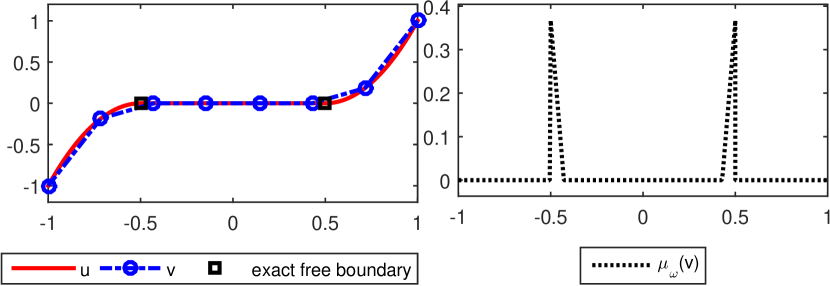
Figure 2: Exact solution $u$ of the two-phase obstacle problem and its approximations $v_{N}$ (left) for $N=8$ and the distributions of $\mu_{\omega}(v_{N})$ (right).

We consider a sequence of approximations

$$v_{N}(x)=I_{N}(u)(x),\quad x\in\left[-1,1\right],$$

where $I_{N}$ (for $N=2,3,\dots$) denotes a piecewise linear nodal interpolant of the function $u$ in $N$ uniformly distributed nodes $\{-1,-1+h,\dots,1-h,1\},$ where $h=2/(N-1)$. Table 2 reports on terms in the energy identity (11) for some increasing values of $N$. In general, it holds

$$\mu_{\omega}(v_{N})=0\qquad\mbox{for }N=4k+1,k\in\mathbb{N}.$$

In these cases, two interpolation nodes lie on the exact free boundary at $x=\pm 0.5$ and sets $\Omega^{-}_{v_{N}},\Omega^{0}_{v_{N}},\Omega^{+}_{v_{N}}$ coincide with $\Omega^{-}_{u},\Omega^{0}_{u},\Omega^{+}_{u}$. For all other approximations $v_{N}$ (see Figure 2 for $N=8$), it holds $\mu_{\omega}(v_{N})>0$. The contribution of the nonlinear measure to the energy identity is measured by the quantity

$$\kappa(v_{N}):=100\,\frac{\mu_{\omega}(v_{N})}{J(v_{N})-J(u)}\quad[\%].$$ (24)

We see in this benchmark, the contribution of $\frac{1}{2}\|\nabla(u-v_{N})\|^{2}_{A}$ dominates over the contribution of the nonlinear measure term $\mu_{\omega}(v_{N})$.

$N$	$\frac{1}{2}\|\nabla(u-v_{N})\|^{2}_{A}$	$\mu_{\omega}(v_{N})$	$J(v_{N})-J(u)$	$\kappa(v_{N})\,[\%]$
2	1.67e+00	2.00e+00	3.67e+00	54.55
5	6.67e-01	00	6.67e-01	0.00
6	3.59e-01	7.20e-02	4.31e-01	16.72
7	2.59e-01	7.41e-02	3.33e-01	22.22
8	2.16e-01	2.62e-02	2.42e-01	10.82
9	1.67e-01	00	1.67e-01	0.00
10	1.20e-01	1.23e-02	1.32e-01	9.33
30	1.23e-02	3.69e-04	1.27e-02	2.91
60	3.06e-03	4.38e-05	3.10e-03	1.41
120	7.53e-04	5.34e-06	7.58e-04	0.70

Table 2: The error identity terms computed for various approximation $v_{N}$.

Acknowledgments.

The first author acknowledges the support of RICAM during Special Semester on Computational Methods in Science and Engineering 2016, Linz, Austria. The second author has been supported by GA CR through the projects GF16-34894L and 17-04301S.

References

- [1] F. Bozorgnia: Numerical solutions of a two-phase membrane problem, Applied Numerical Mathematics 61 (2011), no. 1, 92–107.
- [2] G. Duvaut and G.-L. Lions: Inequalities in mechanics and physics, Springer, Berlin-New York, 1976.
- [3] I. Ekeland and R. Temam, Convex Analysis and Variational Problems, North-Holland, Amsterdam, 1976.
- [4] P. Harasim, J. Valdman: Verification of functional a posteriori error estimates for obstacle problem in 2D. Kybernetika, 50 (6), 978 – 1002, 2014.
- [5] R. H. Nochetto, K. G. Seibert, A. Veeser: Pointwise a posteriori error control for elliptic obstacle problems. Numer. Math., 95, 2003, 631–658.
- [6] S. Repin: A posteriori error estimation for variational problems with uniformly convex functionals. Math. Comp. 69, No. 230, 481–500 (2000).
- [7] S. Repin and J. Valdman: A posteriori error estimates for two-phase obstacle problem, J. Math.Sci. 20, No. 2, 324–336 (2015).
- [8] S. Repin, J. Valdman: Error identities for variational problems with obstacles, arXiv:1702.08689 .
- [9] H. Shahgholian, N. N. Uraltseva, G. S.Weiss: The two-phase membrane problem regularity of the free boundaries in higher dimensions, Int. Math. Res. Not. 2007, No. 8, ID rnm026 (2007).