Probing Higgs self-coupling of a classically scale invariant model
in $e^{+}e^{-}\to Zhh$: Evaluation at physical point

Abstract

A classically scale invariant extension of the standard model predicts large anomalous Higgs self-interactions. We compute missing contributions in previous studies for probing the Higgs triple coupling of a minimal model using the process $e^{+}e^{-}\to Zhh$. Employing a proper order counting, we compute the total and differential cross sections at the leading order, which incorporate the one-loop corrections between zero external momenta and their physical values. Discovery/exclusion potential of a future $e^{+}e^{-}$ collider for this model is estimated. We also find a unique feature in the momentum dependence of the Higgs triple vertex for this class of models.

1 Introduction

The properties of the Higgs boson, now being uncovered through measurements at the LHC experiments, seem to point to an increasingly consistent picture with predictions of the Standard Model (SM) of particle physics. In particular, up to now measured interactions of the Higgs boson with other SM particles agree well with the SM predictions and no sign of significant deviation has been observed [1, 2, 3, 4].

In view of the current status, it would be worth considering a class of models beyond the SM, which possess Higgs portal couplings and at the same time induce the electroweak symmetry breaking via the Coleman–Weinberg (CW) mechanism [5]. On the one hand, in such models anomalies tend to be suppressed in the interactions among the SM particles other than the Higgs boson, as well as in the interactions of the Higgs boson with other SM particles. On the other hand, large anomalies are predicted in the Higgs self-interactions, since the global shape of the Higgs potential [which is given by a $\phi^{4}\log\phi$–type potential at the leading-order (LO)] significantly deviates from that of the SM. Furthermore, this class of models are discussed within the context of dark matter physics [6, 7, 8, 9, 10, 11, 12, 13, 14, 15, 16].

Testability of this class of models has been studied. The CW-type potential predicts a universal value of the three-point Higgs self-coupling from computation of the one-loop effective potential, which is given by $\lambda_{hhh}=5/3\times\lambda_{hhh}^{\rm SM}$ [17, 18, 19]. The large deviation from the SM value can be probed relatively easily using the process $e^{+}e^{-}\to Zhh$ [20] at a future linear collider with the center-of-mass energy around $500$ GeV [21].

There is, however, a caveat in these testability analyses. The value of the above three-point coupling is determined at the zero external momentum limit $p_{i}\to 0$, and this constant value has been used to scale the tree-level $h^{3}$–vertex in the analyses. The CW mechanism is unique in that certain one-loop contributions become comparable to tree-level contributions, the very reason why it is called a radiative symmetry breaking mechanism. This feature applies to the Higgs self-interactions, and one needs to include a part of the one-loop corrections even in the LO analyses, if the proper order counting is respected. According to this order counting the one-loop corrections between $p_{i}=0$ and $p_{i}\sim{\cal O}(m_{t})$ become formally the same order as the three-point coupling determined at $p_{i}\to 0$. Most pessimistically before explicit computation, one could be worried if the large deviation predicted at $p_{i}=0$ may even be almost canceled at the physical values of the external momenta.

In this paper we compute the total and differential cross sections for $e^{+}e^{-}\to Zhh$ in a CW-type Higgs portal model, at the LO of the proper order counting. We take up the minimal model analyzed in ref.[18] which includes $N$ singlet scalar particles and use the order counting developed in ref.[22]. This model has a high predictability because of the small number of model parameters. Let us describe briefly the current status of this model. It is known that this model can be tested by direct dark matter searches [23]. Using the most recent bounds by the XENON1T experiment [24], the model is excluded in the region $N\geq 2$, while the case $N=1$ is marginal. Nevertheless, this test assumes that the reheating temperature of the Universe exceeds the singlet mass scale, and that the dark matter is thermalized. Hence the model cannot be excluded without this assumption, or alternatively, we can put bounds on the reheating temperature ($T\ll m_{s}$). It was also pointed that this model may be tested using $WW$ scattering processes in the future [22].

We show that in this model one-loop corrections induce non-trivial kinematical dependences to the $e^{+}e^{-}\to Zhh$ cross sections, which cannot be accounted for by the constant scaling of the Higgs triple coupling. The kinematical dependence of the $h^{3}$–vertex reflects characteristic features of the model. We also show a general feature valid for CW-type Higgs portal models with more general non-SM sectors.

In Sec. 2 we describe our model and its order counting rule. In Sec. 3 we define an effective Higgs triple coupling. The total and differential cross sections for $e^{+}e^{-}\to Zhh$ are computed in Sec. 4. Conclusion is given in Sec. 5. In A, loop functions are defined. In B, a relation between the $h^{3}$–vertex and the Higgs wave function renormalization is derived using derivative expansion of the effective potential.

2 CSI model

Lagrangian

We consider a model, which has an extended Higgs sector with classical scale invariance (CSI). Throughout the paper we adopt the Landau gauge and dimensional regularization with $d=4-2\epsilon$ space-time dimensions. The bare Lagrangian of the CSI model is given by

$${\cal L}^{\rm CSI}= \,\left[{\cal L}^{\text{SM}}\right]_{\mu^{2}_{\text{H}}\rightarrow 0}+\frac{1}{2}(\partial_{\mu}{\vec{S}_{B}})^{2}-{\lambda^{(B)}_{\text{HS}}}\,(H_{B}^{\dagger}H_{B})(\vec{S}_{B}\cdot\vec{S}_{B})-\frac{\lambda_{S}^{(B)}}{4}(\vec{S}_{B}\cdot\vec{S}_{B})^{2}\,.$$ (1)

$\vec{S}=(S_{1},\cdots,S_{N})^{T}$ denotes a real scalar field, which is a SM singlet and belongs to the $N$ representation of a global $O(N)$ symmetry. The above Lagrangian is invariant under the SM gauge symmetry and the $O(N)$ symmetry and is perturbatively renormalizable. $H$ denotes the doublet Higgs field. Subscripts or superscripts “$B$” in eq. (1) show that the corresponding fields or couplings are the bare quantities. The Higgs interaction terms relevant in our analysis are given by

$${\cal L}^{\rm CSI}_{\text{H--int}} =-\mu^{2\epsilon}(\lambda_{\rm H}+\delta\lambda_{\rm H})(H^{\dagger}H)^{2}-\mu^{2\epsilon}(\lambda_{\rm HS}+\delta\lambda_{\rm HS})H^{\dagger}H\,S_{i}S_{i}\,.$$ (2)

Here we have re-expressed the interaction terms by renormalized quantities and counter-terms: $H$ and $S_{i}$ denote the renormalized fields; $\lambda_{\rm H}$ and $\lambda_{\rm HS}$ represent the renormalized coupling constants; the terms proportional to $\delta\lambda_{\rm H}$ and $\delta\lambda_{\rm HS}$ represent the counter-terms; $\mu$ denotes the renormalization scale.

The Higgs field acquires a non-zero vacuum expectation value (VEV) via the CW mechanism, whereas the singlet field does not [18]. The singlet particles become massive and degenerate (with mass $m_{s}=\lambda_{\rm HS}^{1/2}v$). We expand the Higgs field about the VEV as $H=(G^{+},(v\mu^{-\epsilon}+h+iG^{0})/\sqrt{2})^{T}$ and set $S_{i}=0$, where $h$, $G^{0}$ and $G^{+}$ represent the physical Higgs, neutral- and charged-NG bosons, respectively; $v$ denotes the Higgs VEV. Substituting them into eq. (2), one obtains the Feynman rules for the CSI model.

Order counting: $\xi$ expansion

According to ref.[22] we introduce an auxiliary expansion parameter $\xi$ and rescale the parameters of the model as follows:

$$\lambda_{\rm HS}\rightarrow\xi\,\lambda_{\rm HS}\,,~{}~{}~{}\lambda_{\rm H}\rightarrow\xi^{2}\,\lambda_{\rm H}\,,~{}~{}~{}y_{t}\rightarrow\xi^{1/2}\,y_{t},~{}~{}~{}\mbox{others}\rightarrow{\cal O}(\xi^{2})\,,$$ (3)

where $y_{t}=\sqrt{2}m_{t}/v$ denotes the top-quark Yukawa coupling. Then we expand each physical observable in series expansion in $\xi$, and in the end we set $\xi=1$. If an observable is given as $A(\xi)=\xi^{n}(a_{0}+a_{1}\xi+a_{2}\xi^{2}+\dots)$, we define the LO term of $A$ as $a_{0}$, the next-to-leading order (NLO) term of $A$ as $a_{1}$, etc. From previous experiences we expect the size of the effective expansion parameter in these series expansions to be order 10–30%, depending on the observables. It follows from the above counting that $m_{h}^{2}\sim{\cal O}(\xi^{2})$ and $m_{t}^{2},m_{s}^{2}\sim{\cal O}(\xi)$. The reason for assigning $\xi^{2}$ to the other couplings (in particular to the electroweak gauge couplings) will be made clear below.

Determination of parameters

Following Sec. II of ref.[22], we can determine $\lambda_{\rm H}$ and $\lambda_{\rm HS}$ from the tadpole condition and the on-shell Higgs mass condition in terms of VEV $v=246.6~{}{\rm GeV}$, the Higgs mass $m_{H}=125.03\pm 0.27~{}{\rm GeV}$ [25, 26] and the top-quark mass $m_{t}=173.34\pm 0.76~{}{\rm GeV}$ [27]. $\lambda_{\rm H}$ and $\delta\lambda_{\rm H}$ depend on renormalization scheme; if the counter-terms are defined by the $\overline{\rm MS}$ scheme,

$$\lambda_{\rm H} = \frac{N\lambda_{\rm HS}}{16\pi^{2}}\left(1-\ln[\lambda_{\rm HS}v^{2}/\mu^{2}]\right)-\frac{3y_{t}^{4}}{16\pi^{2}}\left(1-\ln[y_{t}^{4}v^{2}/(2\mu^{2})]\right),$$ (4)

$$\delta\lambda_{\rm H} = \frac{1}{\epsilon}\left(\frac{N\lambda_{\rm HS}}{16\pi^{2}}-\frac{3y_{t}^{4}}{16\pi^{2}}\right).$$ (5)

The on-shell Higgs mass condition is given by

$$\Sigma(m_{h}^{2})=0,$$ (6)

where $\Sigma(q^{2})$ denotes the Higgs self-energy, counted as ${\cal O}(\xi^{2})$, whose order is the same as $m_{h}^{2}$. The analytic expression of $\Sigma(q^{2})$ is given in ref.[22]. The values of $\lambda_{\rm HS}$ and $m_{s}$ determined by eq. (6) and $v=246.6$GeV are summarized in Table 1.

$N$	$1$	$4$	12
$\lambda_{\rm HS}$	$4.87$	$2.45$	$1.42$
$m_{s}~{}{\rm GeV}$	543	385	293

Table 1: Values of $\lambda_{\rm HS}$ and $m_{s}$ for $N=1,~{}4,~{}12$

3 Higgs triple coupling

We define an effective Higgs triple coupling for $h^{*}\to hh$ as

$$\lambda_{hhh}(q^{2})=\frac{q^{2}-m_{h}^{2}}{q^{2}-m_{h}^{2}-\Sigma_{h}(q^{2})}\times\frac{1}{v}\Gamma_{hhh}(q^{2}),$$ (7)

where $\Gamma_{hhh}(q^{2})$ denotes the 1PI three-point vertex of the Higgs boson, see Fig. 1.

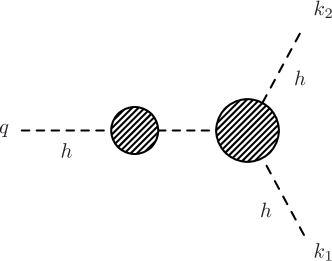
Figure 1: Schematic diagram for the effective Higgs triple coupling for $h^{*}\to hh$.

The two external Higgs bosons corresponding to the final state are taken to be on-shell, while the invariant mass $q$ of the initial (off-shell) Higgs boson is taken as a variable.

The diagrams contributing to $\Gamma_{hhh}(q^{2})$ are shown in Fig. 2.

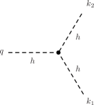
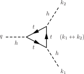
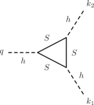
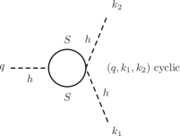
Figure 2: Diagrams contributing to $\Gamma_{hhh}(q^{2})$ at LO.

Its analytic expression is given by

$$\frac{1}{v}\Gamma_{hhh}(q^{2}) = 6(\lambda_{H}+\delta\lambda_{H})$$ (8)

$$+\frac{3m_{t}y_{t}^{3}}{4\sqrt{2}\pi^{2}v}B_{0}\left(q^{2},m_{t}^{2},m_{t}^{2}\right)+\frac{3m_{t}y_{t}^{3}}{2\sqrt{2}\pi^{2}v}B_{0}\left(0,m_{t}^{2},m_{t}^{2}\right)$$

$$-\frac{3m_{t}y_{t}^{3}}{8\sqrt{2}\pi^{2}v}(q^{2}-8m_{t}^{2})C_{0}\left(q^{2},0,0,m_{t}^{2},m_{t}^{2},m_{t}^{2}\right)$$

$$-\frac{N\lambda_{\text{HS}}^{2}}{8\pi^{2}}B_{0}\left(q^{2},m_{s}^{2},m_{s}^{2}\right)-\frac{N\lambda_{\text{HS}}^{2}}{4\pi^{2}}B_{0}\left(0,m_{s}^{2},m_{s}^{2}\right)$$

$$-\frac{N\lambda_{\text{HS}}^{3}v^{2}}{2\pi^{2}}C_{0}\left(q^{2},0,0,m_{s}^{2},m_{s}^{2},m_{s}^{2}\right),$$

where $B_{0}\left(p^{2},m^{2},m^{2}\right)$ and $C_{0}\left(p_{1}^{2},p^{2}_{2},p^{2}_{3},m^{2},m^{2},m^{2}\right)$ represent loop functions defined in A. $\Sigma(q^{2})$ and $\Gamma(q^{2})$ do not depend on the renormalization scale $\mu^{2}$, due to cancellation between $\lambda_{\rm H}$ and loop functions. We can use $\lambda_{hhh}(q^{2})/\lambda_{hhh}^{\rm SM,tree}$ to scale the tree-level SM Higgs three-point vertex in the Higgs exchange diagram for $e^{+}e^{-}\to Zhh$.

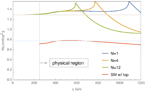
(a)

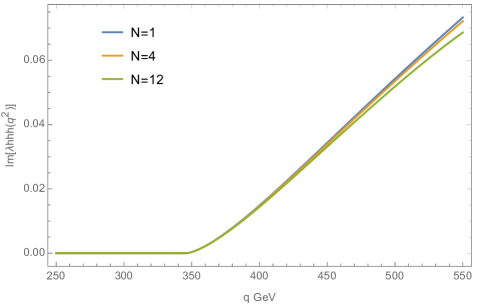
(b)

Figure 3: (a) ${\rm Re}\,\lambda_{hhh}(q^{2})$ at LO (blue ($N=1$), orange ($N=4$), green ($N=12$)) vs. $q$. Also shown are $\lambda_{hhh}$ as determined from the one-loop effective potential (light brown) and ${\rm Re}\,\lambda_{hhh}^{\rm SM}$ tree (light blue) and including the tree plus top-quark one-loop contributions (red). Physical region, indicated by the arrow, corresponds to $2m_{h}\leq q$. (b) Same as (a) but for ${\rm Im}\,\lambda_{hhh}(q^{2})$.

We show the real and imaginary parts of $\lambda_{hhh}(q^{2})$ as functions of $q$ in Figs. 3 a,b. We use eq. (7) to make the plot. For comparison we also show $\lambda_{hhh}$ as determined from the one-loop effective potential, $\frac{5}{3}\lambda^{\rm SM}_{hhh}$, which corresponds to setting all the external momenta to zero. By comparison we see non-trivial $q^{2}$ dependence in $\lambda_{hhh}(q^{2})$. In the same figures we also show $\lambda_{hhh}^{\rm SM}$ including the tree plus top-quark one-loop contribution, where the $q^{2}$ dependence stems from the top-loop contribution. The top-quark loop contribution raises the couplings at $q\hbox{ \raise 3.0pt\hbox to0.0pt{$>$}\raise-3.0pt\hbox{$\sim$} }2m_{t}$, which is common in the SM and CSI model.

It is useful to examine $q^{2}$ expansion of $\lambda_{hhh}(q^{2})$ for model identification. $q^{2}$ expansion is reasonable for singlet contribution at $q\simeq 2m_{h}$, because $q^{2}/m_{s}^{2}\ll 1$. We show in B, using derivative expansion of the effective action, that the coefficient of the $q^{2}$ term of this expansion is determined by the divergent part of the wave function renormalization for the Higgs boson in a general CSI-model. Since the singlet-loop does not contribute to the divergent part of the Higgs wave function renormalization, there is no $q^{2}$ term from the singlet-loop in $\lambda_{hhh}(q^{2})$. The absence of $q^{2}$ term in the singlet contribution is also confirmed by an explicit calculation of $\Gamma_{hhh}$:

$$-\frac{N\lambda_{\text{HS}}^{2}}{8\pi^{2}}B_{0}\left(q^{2},m_{s}^{2},m_{s}^{2}\right)-\frac{N\lambda_{\text{HS}}^{2}}{4\pi^{2}}B_{0}\left(0,m_{s}^{2},m_{s}^{2}\right)-\frac{N\lambda_{\text{HS}}^{3}v^{2}}{2\pi^{2}}C_{0}\left(q^{2},0,0,m_{s}^{2},m_{s}^{2},m_{s}^{2}\right)$$ (9)

$$= ({\rm const.})+\left[\frac{1}{6}\frac{N\lambda_{\text{HS}}^{2}}{8\pi^{2}}-\frac{1}{24m_{s}^{2}}\frac{N\lambda_{\text{HS}}^{3}v^{2}}{2\pi^{2}}\right]\left(\frac{q^{2}}{m_{s}^{2}}\right)+\left[\frac{1}{60}\frac{N\lambda_{\text{HS}}^{2}}{4\pi^{2}}-\frac{1}{180m_{s}^{2}}\frac{N\lambda_{\text{HS}}^{3}v^{2}}{2\pi^{2}}\right]\left(\frac{q^{2}}{m_{s}^{2}}\right)^{2}+\cdots$$

$$= ({\rm const.})+0\times\frac{q^{2}}{m_{s}^{2}}+\frac{N\lambda^{2}_{\rm HS}}{1440\pi^{2}}\left(\frac{q^{2}}{m_{s}^{2}}\right)^{2}+\cdots.$$

See eq.(8). In the third line, $m_{s}^{2}=\lambda_{\rm HS}v^{2}$ is used. Thus, the $q^{2}$ dependence starts at order $q^{4}$ for the singlet contribution. On the other hand, since the top-quark contributes to the divergent part of the Higgs wave function renormalization, the $q^{2}$ term of $\lambda_{hhh}(q^{2})$ stems solely from the top-quark contribution at LO. This is why $N$ dependence is almost absent until very close to the singlet-pair threshold in Fig. 3 a,b. Hence, using this unique feature of CSI models, we can test the origin if the anomaly by looking at the behavior of the Higgs triple coupling near the Higgs pair threshold.

4 $e^{+}e^{-}\to Zhh$ cross sections

In the SM there are four tree-level diagrams which contribute to the process $e^{+}e^{-}\to Zhh$. See Fig. 4.

Figure 4: Diagrams which contribute to $e^{+}e^{-}\to Zhh$.

One of the diagrams contains the Higgs three-point vertex, while the other three diagrams contribute as irreducible background diagrams for probing the triple Higgs coupling. To compute the cross section for the CSI model, we replace the tree-level $\lambda_{hhh}^{\rm SM}$ by $\lambda_{hhh}(q^{2})$. The background diagrams and the signal diagram are counted as the same order in $\xi$ since we assign $\xi^{2}$ to the electroweak gauge couplings. Numerically this order counting is reasonable.

We calculate the total and differential cross sections using MadGraph5 [28], with the initial $e^{\pm}$ longitudinal polarizations $P(e^{+},e^{-})=(0.3,-0.8)$. At $\sqrt{s}=500$ GeV, the total cross section is evaluated to be $\sigma^{\rm CSI}_{\rm tot}(e^{+}e^{-}\to Zhh)=0.341$ fb. This amounts to $+47$% deviation compared to the tree-level SM total cross section. We show the $\sqrt{s}$ dependence of the total cross section in Fig. 5. The deviation of the total cross section from the tree-level SM prediction decreases as $\sqrt{s}$ increases.

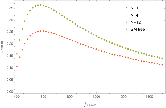
Figure 5: Total cross section $\sigma$ for $e^{+}e^{-}\to Zhh$ vs. $\sqrt{s}$ at SM (red), $N=1$ (blue), $N=4$ (orange),$N=12$ (green).

We also compute $d\sigma/dq$ at $\sqrt{s}=500$ GeV for $N=1$ and at several $\sqrt{s}$ between $600-1200$ GeV for $N=12$, where $q^{2}=m_{hh}^{2}=(p_{1}+p_{2})^{2}$. The results are shown in Figs. 6 and 7.

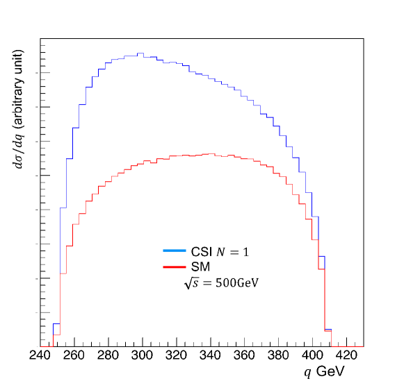
Figure 6: Differential cross section $d\sigma/dq$ at $\sqrt{s}=500$ GeV for $e^{+}e^{-}\to Zhh$, where $q^{2}=(p_{h1}+p_{h2})^{2}$. $d\sigma/dq$ is non-zero only in $2m_{h}\leq q\leq\sqrt{s}-m_{Z}$.

The kinematically allowed range is given by $2m_{h}\leq q\leq\sqrt{s}-m_{Z}$. In Fig. 6, the enhancement from the SM prediction in the low $q$ region is due to the enhancement of the triple Higgs coupling at low $q$. The relative enhancement factor decreases as $q$ increases, since the relative weight of the signal diagram is reduced due to rapid decrease of the Higgs propagator $1/(q^{2}-m_{h}^{2}-\Sigma_{h})$. In Fig. 7, no peak is visible corresponding to the singlet pair creation at $q\simeq 2m_{s}(\simeq 600{\rm GeV})$, because of the suppression by the Higgs propagator. The difference between the prediction using $\lambda_{hhh}(q^{2})$ and $\lambda_{hhh}=\frac{5}{3}\lambda^{\rm SM}_{hhh}$ determined from the effective potential, is found in small $q$ region in the $N=12$ case. From these figures we see that it is challenging to detect different $q$-dependences, which would require huge statistics.

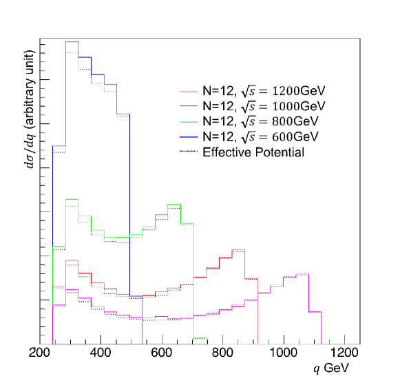
Figure 7: Differential cross sections $d\sigma/dq$ at $N=12$, $\sqrt{s}=600({\rm blue})$, $800({\rm green})$, $1000({\rm red})$ and $1200({\rm magenta})$ GeV for $e^{+}e^{-}\to Zhh$, where $q^{2}=(p_{h1}+p_{h2})^{2}$. Black dotted lines show the same cross sections using $\lambda_{hhh}$ determined from the effective potential.

Integrated luminosity necessary for a discovery at $5\sigma$ (an exclusion at $3\sigma$) of this model is estimated to be $710~{}{\rm fb}^{-1}$ ($260~{}{\rm fb}^{-1}$) at $\sqrt{s}=500{\rm GeV}$. This estimation uses the number of signal and background events from the full simulation of International Linear Collider (ILC) experiment given in ref.[29] for $e^{+}e^{-}\to Zhh$, $h\to b\bar{b}$ process and $m_{h}=120$GeV at $\sqrt{s}=500$GeV, with events corresponding to $2{\rm ab}^{-1}$. We rescaled the number of the signal event $N_{\rm sig}$ by the ratio of the total cross sections and of the branching ratios for $h\to b\bar{b}$ as

$$N_{\rm sig}\to N^{\rm CSI}_{\rm sig}=(\sigma^{\rm CSI}_{\rm tot}/\sigma^{\rm SM}_{\rm tot})(Br^{m_{h}=125{\rm GeV}}_{h\to b\bar{b}}/Br^{m_{h}=120{\rm GeV}}_{h\to b\bar{b}})^{2}N_{\rm sig},$$ (10)

while the $1\sigma$ standard deviation is approximated by $N_{\rm sig}/\sqrt{N_{\rm BG}}$.

To end this section we give some discussion. The $W$-fusion process is another process at ILC to measure the triple Higgs coupling and is the dominant process at $\sqrt{s}\gtrsim 1200$GeV in SM. It turns out that the total cross section of this process decreases as the triple Higgs coupling increases due to a negative interference [30], while the $Zhh$ cross section are enhanced by positive interference. As a result it is advantageous to analyze $e^{+}e^{-}\to Zhh$ rather than $W$-fusion process for the CSI model.

It is pointed that this model has a Landau pole around $3.5~{}{\rm TeV}~{}(N=1)$, $16~{}{\rm TeV}~{}(N=4)$ and $28~{}{\rm TeV}~{}(N=12)$ at LO [18]. The existence of the Landau pole indicates that perturbative expansion of the model does not work around its scale or the model turns into some UV theory. Perturbative validity has been discussed in the leading-logarithmic analyses of the effective potential and $WW$-scattering amplitude [22]. Since our analysis deals with the energy scale well below the Landau pole, we consider that the perturbative analysis given in this paper is justified, where we regard this model as an effective theory valid around $\mathcal{O}(100{\rm GeV})$.

5 Conclusion

In the minimal CSI model, we have incorporated the one-loop corrections between the zero external momenta and physical point in the total and differential cross sections for $e^{+}e^{-}\to Zhh$. We find that the bulk of the large anomaly predicted at the zero-external-momentum limit remains, while a non-trivial $q^{2}$ dependence of the Higgs triple interaction is induced. We also find that at LO, the effect of the singlet scalar boson has no $q^{2}$ term in $q^{2}$ expansion of the Higgs triple coupling. This feature does not depend on the number or mass spectrum of the singlet scalars and is a general feature of CW-type models with singlet scalar bosons, as shown in B. The top loop effects induce a non-negligible $q^{2}$ dependence, in accord with the expectation based on order counting. In contrast, $N$-dependent effects by the singlet-loop are found to remain small below the singlet pair threshold due to this unique feature of the $q^{2}$ expansion. We have estimated sensitivity of the $e^{+}e^{-}\to Zhh$ total cross section to the deviation from the SM and found that it is fairly promising.

Appendix A Loop functions

The loop functions used in Sec. 3 are defined as follows. Here, $d=4-2\epsilon$, $\mu$ represents the renormalization scale, and $\kappa=(2\pi\mu)^{2\epsilon}/(i\pi^{2})$:

$$B_{0}(p^{2},m^{2},m^{2}) = \kappa\int\frac{d^{d}q}{[q^{2}-m^{2}][(q+p)^{2}-m^{2}]},$$ (11)

$$C_{0}(p_{1}^{2},p_{2}^{2},p_{3}^{2},m^{2},m^{2},m^{2}) = \kappa\int\frac{d^{d}q}{[q^{2}-m^{2}][(q+p_{1})^{2}-m^{2}][(q+p_{2})^{2}-m^{2}]}.$$ (12)

These can be expressed as

$$B_{0}(p^{2},m^{2},m^{2}) = \frac{1}{\bar{\epsilon}}+\ln[\mu^{2}]-\int^{1}_{0}dx\ln[m^{2}-x(1-x)p^{2}-i0],$$ (13)

$$C_{0}(p_{1}^{2},p_{2}^{2},p_{3}^{2},m^{2},m^{2},m^{2})=\int^{1}_{0}dx\int^{1-x}_{0}\!\!\!\!\!dy[m^{2}-x(1-x)p_{1}^{2}+xy(p^{2}_{3}-p^{2}_{1}-p^{2}_{2})-y(1-y)p_{2}^{2}-i0]^{-1},$$ (14)

where $p_{1}+p_{2}+p_{3}=0$, and $1/\bar{\epsilon}=1/\epsilon-\gamma+\ln[4\pi]$ ($\gamma=0.5772\cdots$ denotes Euler’s number).

The expansion of $B_{0}(p^{2},m^{2},m^{2})$ and $C_{0}(p^{2},0,0,m^{2},m^{2},m^{2})$ in $p^{2}$ are given by

$$B_{0}(p^{2},m^{2},m^{2}) = \frac{1}{\bar{\epsilon}}-\ln\left(\frac{m^{2}}{\mu^{2}}\right)-\frac{1}{6}\left(\frac{p^{2}}{m^{2}}\right)-\frac{1}{60}\left(\frac{p^{2}}{m^{2}}\right)^{2}+\cdots,$$ (15)

$$C_{0}(p^{2},0,0,m^{2},m^{2},m^{2}) = \frac{1}{2m^{2}}+\frac{1}{24m^{2}}\left(\frac{p^{2}}{m^{2}}\right)+\frac{1}{180m^{2}}\left(\frac{p^{2}}{m^{2}}\right)^{2}+\cdots.$$ (16)

Appendix B Expansion of effective action and momentum dependence of $\lambda_{hhh}(q^{2})$

We consider a general CSI model. The derivative expansion of the effective action in terms of classical Higgs field $\Phi$ in the symmetric phase is given by

$$\Gamma[\Phi] = -V(\Phi^{{\dagger}}\Phi)$$ (17)

$$+(\partial_{\mu}\Phi)^{{\dagger}}(\partial_{\mu}\Phi)~{}\Gamma^{1,1}[\Phi^{{\dagger}}\Phi]+\Phi^{{\dagger}}(\partial^{2}\Phi)\Gamma^{1,2}[\Phi^{{\dagger}}\Phi]$$

$$+((\partial_{\mu}\Phi)^{{\dagger}}(\partial_{\mu}\Phi))^{2}~{}\Gamma^{2,1}[\Phi^{{\dagger}}\Phi]+\cdots,$$

where $V(\Phi^{{\dagger}}\Phi)$ is the effective potential and $\Gamma^{n,i}[\Phi^{{\dagger}}\Phi]$ denotes the coefficient of the $i^{\rm th}$ term of $2n^{\rm th}$ derivative terms. The mass dimension of $\Gamma^{n,i}[\Phi^{{\dagger}}\Phi]$ is equal to $4-4n$. By setting $\Phi\to(0,(v+h)/\sqrt{2})$, the $q^{2}$ term of the physical Higgs ($h$) three-point function stems from

$$(\partial_{\mu}\Phi)^{{\dagger}}(\partial_{\mu}\Phi)~{}\Gamma^{1,1}[\Phi^{{\dagger}}\Phi] \ni \left.\frac{\delta\Gamma^{1,1}[(v+h)^{2}/2]}{\delta h}\right|_{h\to 0}(\partial_{\mu}h)^{2}h,$$ (18)

$$\Phi^{{\dagger}}(\partial^{2}\Phi)\Gamma^{1,2}[\Phi^{{\dagger}}\Phi] \ni \left.\frac{\delta\Gamma^{1,2}[(v+h)^{2}/2]}{\delta h}\right|_{h\to 0}(\partial^{2}h)h^{2}.$$ (19)

Hence, the $q^{2}$ term of three point function is defined by $\Gamma^{1,i}$. On the other hand, $\left.\Gamma^{1,i}[\Phi^{{\dagger}}\Phi]\right|_{\Phi\to(0,(v+h)/\sqrt{2})}$ determine the Higgs wave function renormalization $Z$,

$${\mathcal{L}}\ni\frac{1}{2}Z(\partial_{\mu}h)(\partial_{\mu}h).$$ (20)

This means that the $q^{2}$ term of the three-point function is controlled by the wave function renormalization.

In a general CSI-model, the form of $\Gamma^{1,i}$ is fixed at LO by the following argument. Since the bare Lagrangian has classical scale invariance, the effective action has only the classical field $\Phi$ and renormalization scale $\mu^{2}$ as dimensionful parameters, and since $\mu^{2}$ always appears in the logarithm, the form of $\Gamma^{1,i}$ is given by

$$\Gamma^{1,i}[\Phi^{{\dagger}}\Phi]=a^{i}+b^{i}\ln(\Phi^{{\dagger}}\Phi/\mu^{2}),$$ (21)

where $a^{i}$ and $b^{i}$ represent dimensionless constants determined by coupling constants. $a^{i}$ does not contain $\Phi$, only the logarithmic term contributes to eqs.(18,19). Furthermore, $\ln(\mu^{2})$ is associated with the $1/\epsilon$ part of the wave function renormalization.

The above argument does not apply to models with dimensionful parameters such as $m^{2}$, since polynominal of $\Phi^{{\dagger}}\Phi/m^{2}$ contributes to eq.(21).

In this paper, we consider a CSI model with SM gauge singlet scalar bosons. Since the VEV of the singlet bosons is equal to zero, the previous argument applies and the contribution of the singlet-loops is expressed by eq.(21). Noting that the wave function renormalization by the singlet-loop is finite $(a^{i}<\infty,~{}b^{i}=0)$ , the singlet bosons do not contribute to the $q^{2}$ term of the three-point function.

On the other hand, the fermion and vector bosons, e.g. the top, $W$ and $Z$, contribute to the divergent part of the Higgs wave function renormalization since the mass dimension of a fermion propagator is equal to $-1$ and $VVh$ has derivative couplings. As a result, fermions and vector bosons generally contribute to the $q^{2}$ term of the Higgs three-point function.

References

References

- [1] M. Aaboud et al. [ATLAS Collaboration], “Search for additional heavy neutral Higgs and gauge bosons in the ditau final state produced in 36 fb-1 of collisions at = 13 TeV with the ATLAS detector”, [arXiv:1709.07242 [hep-ex]].
- [2] V. Khachatryan et al. [CMS Collaboration], “Search for the associated production of the Higgs boson with a top-quark pair”, JHEP 1409, 087 (2014), [arXiv:1408.1682 [hep-ex]].
- [3] G. Aad et al. [ATLAS Collaboration], “Search for the associated production of the Higgs boson with a top quark pair in multilepton final states with the ATLAS detector”, Phys. Lett. B 749, 519 (2015), [arXiv:1506.05988 [hep-ex]].
- [4] CMS Collaboration [CMS Collaboration], “Search for Higgs boson production in association with top quarks in multilepton final states at ”, CMS-PAS-HIG-17-004.
- [5] S. R. Coleman and E. J. Weinberg, “Radiative Corrections as the Origin of Spontaneous Symmetry Breaking”, Phys. Rev. D 7, 1888 (1973).
- [6] C. P. Burgess, M. Pospelov and T. ter Veldhuis, “The Minimal model of nonbaryonic dark matter: A Singlet scalar”, Nucl. Phys. B 619, 709 (2001), [hep-ph/0011335].
- [7] P. Ghosh, A. K. Saha and A. Sil, “Study of Electroweak Vacuum Stability from Extended Higgs Portal of Dark Matter and Neutrinos”, arXiv:1706.04931 [hep-ph].
- [8] V. Silveira and A. Zee, “Scalar Phantoms”, Phys. Lett. 161B, 136 (1985).
- [9] J. McDonald, “Gauge singlet scalars as cold dark matter”, Phys. Rev. D 50, 3637 (1994), [hep-ph/0702143 [HEP-PH]].
- [10] J. M. Cline, K. Kainulainen, P. Scott and C. Weniger, “Update on scalar singlet dark matter”, Phys. Rev. D 88, 055025 (2013), [arXiv:1306.4710 [hep-ph]].
- [11] W. L. Guo and Y. L. Wu, “The Real singlet scalar dark matter model”, JHEP 1010, 083 (2010), [arXiv:1006.2518 [hep-ph]].
- [12] K. Endo and K. Ishiwata, “Direct detection of singlet dark matter in classically scale-invariant standard model,” Phys. Lett. B 749, 583 (2015) [arXiv:1507.01739 [hep-ph]].
- [13] K. Ishiwata, Phys. Lett. B 710, 134 (2012) doi:10.1016/j.physletb.2012.02.048 [arXiv:1112.2696 [hep-ph]].
- [14] M. Heikinheimo, A. Racioppi, M. Raidal, C. Spethmann and K. Tuominen, “Physical Naturalness and Dynamical Breaking of Classical Scale Invariance,” Mod. Phys. Lett. A 29, 1450077 (2014) [arXiv:1304.7006 [hep-ph]].
- [15] E. Gabrielli, M. Heikinheimo, K. Kannike, A. Racioppi, M. Raidal and C. Spethmann, “Towards Completing the Standard Model: Vacuum Stability, EWSB and Dark Matter,” Phys. Rev. D 89, no. 1, 015017 (2014) [arXiv:1309.6632 [hep-ph]].
- [16] H. Davoudiasl and I. M. Lewis, “Right-Handed Neutrinos as the Origin of the Electroweak Scale,” Phys. Rev. D 90, no. 3, 033003 (2014) [arXiv:1404.6260 [hep-ph]].
- [17] D. Chway, T. H. Jung, H. D. Kim and R. Dermisek, “Radiative Electroweak Symmetry Breaking Model Perturbative All the Way to the Planck Scale”, Phys. Rev. Lett. 113, no. 5, 051801 (2014), [arXiv:1308.0891 [hep-ph]].
- [18] K. Endo and Y. Sumino, “A Scale-invariant Higgs Sector and Structure of the Vacuum”, JHEP 1505, 030 (2015), [arXiv:1503.02819 [hep-ph]].
- [19] K. Hashino, S. Kanemura and Y. Orikasa, “Discriminative phenomenological features of scale invariant models for electroweak symmetry breaking”, Phys. Lett. B 752, 217 (2016), [arXiv:1508.03245 [hep-ph]].
- [20] G. J. Gounaris, D. Schildknecht and F. M. Renard, Phys. Lett. 83B, 191 (1979). doi:10.1016/0370-2693(79)90683-X
- [21] T. Barklow, K. Fujii, S. Jung, M. E. Peskin and J. Tian, “Model-Independent Determination of the Triple Higgs Coupling at e+e- Colliders”, [arXiv:1708.09079 [hep-ph]].
- [22] K. Endo, K. Ishiwata and Y. Sumino, “ scattering in a radiative electroweak symmetry breaking scenario”, Phys. Rev. D 94, no. 7, 075007 (2016), [arXiv:1601.00696 [hep-ph]].
- [23] J. McKay [GAMBIT Collaboration], “Global fits of the scalar singlet model using GAMBIT”, [arXiv:1710.02467 [hep-ph]].
- [24] E. Aprile et al. [XENON Collaboration], “First Dark Matter Search Results from the XENON1T Experiment”, [arXiv:1705.06655 [astro-ph.CO]].
- [25] G. Aad et al. [ATLAS Collaboration], “Measurement of the Higgs boson mass from the and channels with the ATLAS detector using 25 fb-1 of collision data”, Phys. Rev. D 90, no. 5, 052004 (2014), [arXiv:1406.3827 [hep-ex]].
- [26] V. Khachatryan et al. [CMS Collaboration], “Observation of the diphoton decay of the Higgs boson and measurement of its properties”, Eur. Phys. J. C 74, no. 10, 3076 (2014), [arXiv:1407.0558 [hep-ex]].
- [27] [ATLAS and CDF and CMS and D0 Collaborations], “First combination of Tevatron and LHC measurements of the top-quark mass”, arXiv:1403.4427 [hep-ex].
- [28] J. Alwall et al., “The automated computation of tree-level and next-to-leading order differential cross sections, and their matching to parton shower simulations”, JHEP 1407, 079 (2014), [arXiv:1405.0301 [hep-ph]].
- [29] J. Tian, “Study of Higgs self-coupling at the ILC based on the full detector simulation at GeV and TeV”,
- [30] J. Tian et al. [ILD Collaboration], “Measurement of Higgs couplings and self-coupling at the ILC”, PoS EPS -HEP2013, 316 (2013), [arXiv:1311.6528 [hep-ph]].