The magnetic dipole-dipole interaction induced by electromagnetic field

Abstract

We give a derivation for the indirect interaction between two magnetic dipoles induced by the quantized electromagnetic field. It turns out that the interaction between permanent dipoles directly returns to the classical form; the interaction between transition dipoles does not directly return to the classical result, yet returns in the short-distance limit. In a finite volume, the field modes are highly discrete, and both the permanent and transition dipole-dipole interactions are changed. For transition dipoles, the changing mechanism is similar with the Purcell effect, since only a few number of nearly resonant modes take effect in the interaction mediation; for permanent dipoles, the correction comes from the boundary effect: if the dipoles are placed close to the boundary, the influence is strong, otherwise, their interaction does not change too much from the free space case.

I Introduction

The interaction between particles is induced by their local interaction with the field. This is a basic understanding in modern physics, and should also applies for the interaction between two electric/magnetic dipoles. Thus, by controlling the property of the electromagnetic (EM) field, one can artificially engineer the dipole-dipole interaction Liao and Zubairy (2014); Liao et al. (2015); Lambert et al. (2016); Baranov et al. (2016); Liao et al. (2016); Shahmoon and Kurizki (2013a, b); Cai et al. (2016); Shahmoon (2017); Donaire et al. (2017); Cortes and Jacob (2017), which widely appears in many different microscopic systems, such as the interaction between the Josephson qubit and the dielectric defects Martinis et al. (2005); Paik et al. (2011); Rigetti et al. (2012); Lisenfeld et al. (2016), the interaction between the nitrogen-vacancy and the nuclear spins around Doherty et al. (2013); Zhao et al. (2012), as well as the dipoles in chemical and biology molecular Yang et al. (2010); El-Ganainy and John (2013); Dong et al. (2016).

In classical electrodynamics, the interactions between two electric/magnetic dipoles are given by Jackson (1998)

$$V_{\mathrm{e}} =\frac{1}{4\pi\epsilon_{0}}\frac{\vec{p}_{1}\cdot\vec{p}_{2}-3(\vec{p}_{1}\cdot\hat{\mathrm{e}}_{\mathbf{r}})(\vec{p}_{2}\cdot\hat{\mathrm{e}}_{\mathbf{r}})}{r^{3}},$$

$$V_{\mathrm{m}} =\frac{\mu_{0}}{4\pi}\frac{\vec{m}_{1}\cdot\vec{m}_{2}-3(\vec{m}_{1}\cdot\hat{\mathrm{e}}_{\mathbf{r}})(\vec{m}_{2}\cdot\hat{\mathrm{e}}_{\mathbf{r}})}{r^{3}}.$$ (1)

Thus it is natural to expect such interaction can be derived using quantum mechanics, based on the idea of the mediation of the quantized EM field.

The field induced interaction between two electric dipoles has been studied based on both the Heisenberg equation Lyuboshitz (1968); Lehmberg (1970); Ficek et al. (1987) and the master equation Agarwal (1974); Ficek and Swain (2005). In these studies, two resonant electric dipoles with the same transition frequency are concerned, and an interaction Hamiltonian $\hat{H}_{\mathrm{e}}=\xi(\hat{\sigma}_{1}^{+}\hat{\sigma}_{2}^{-}+\hat{\sigma}_{1}^{-}\hat{\sigma}_{2}^{+})$ is derived from the mediation of the field. The interaction strength $\xi$ does not directly return to the above classical result, but returns in the short-distance limit $r/\lambda\ll 1$ Dicke (1954), where $r$ is the distance between the two dipoles, and $\lambda$ is the wavelength of the transition frequency.

Notice that there is also some conceptual difficulty when studying the electric dipole interaction induced by the EM field, i.e., the static electric interaction is induced by the longitudinal modes of the EM field, which are not quantized in the Coulomb gauge Agarwal (1974); Cohen-Tannoudji et al. (1989). If the Lorenz gauge is adopted, some other conceptual difficulties, e.g., the negative probability problem, also arise Ryder (1996), which makes it uneasy to get a clear picture on this problem.

On the contrast, the magnetic interaction only involves the transverse modes of the EM field, which can be well quantized under the Coulomb gauge, thus it could be clear to study the magnetic dipole-dipole interaction Baranov et al. (2016); Lambert et al. (2016). In this paper, we give a simple derivation for this indirect interaction between two magnetic dipoles induced by the EM field. Our derivation goes through the following procedure:

1) First, only dipole-1 is put in the EM field, and that generates a dipole field.

2) The magnetic field contains both the vacuum field and the dipole field, and the interaction between dipole-2 and the dipole field leads to the dipole-dipole interaction.

Based on this idea, we obtain an interaction Hamiltonian for the two magnetic dipoles, which is formally exact and naturally has a retarded structure. After proper Markovian approximation and rotating-wave approximation (RWA), the interaction reduces to a time-local one.

Here we concern both the permanent dipole and transition dipole, which correspond to the diagonal and off-diagonal elements of the dipole operator respectively. Our result shows that, in free space, the interaction between the permanent dipoles directly returns to the classical interaction; the interaction between transition dipoles has the same form with the previous studies on electric dipole interaction Agarwal (1974); Lehmberg (1970); Ficek et al. (1987), and it does not directly return to the classical result, but returns in the limit $r/\lambda\ll 1$.

We also study the dipole-dipole interaction in a finite volume, where the field modes are highly discrete. Both the permanent and transition dipole-dipole interactions are changed from the free space case, but by different mechanisms. For transition dipoles, this changing mechanism is similar with the Purcell effect Purcell et al. (1946); Scully and Zubairy (1997), since only a few number of nearly resonant modes take effect in the mediation of the interaction; for permanent dipoles, still all the field modes take effect for the interaction mediation, and the correction comes from the boundary effect: if the dipoles are placed close to the boundary, the influence is strong, if they are both placed far away from the boundary, their interaction does not change too much from the free space case, and this is also similar with the situation in classical electrodynamics.

The paper is arranged as follows: in Sec. II, we derive the retarded dipole-dipole interaction which is formally exact. In Sec. III, proper approximations are made and the time-local interaction is obtained. In Sec. IV, we study the dipole-dipole interaction in a finite volume. Finally, we draw summary in Sec. V. Some calculation details are presented in the Appendices.

II Retarded interaction between two magnetic dipoles

We first consider there are two magnetic dipoles fixed in the EM field, and the total Hamiltonian is $\hat{{\cal H}}=\hat{H}_{1}+\hat{H}_{2}+\hat{H}_{\text{{em}}}+\hat{H}_{\mathrm{int}}$. Here $\hat{H}_{1,2}$ are self-Hamiltonians of the two dipoles, which are modeled as two-level systems ($|\mathsf{g}_{i}\rangle$, $|\mathsf{e}_{i}\rangle$), and $\hat{H}_{i}=\hbar\Omega_{i}|\mathsf{e}_{i}\rangle\langle\mathsf{e}_{i}|$ for $i=1,2$. $\hat{H}_{\text{{em}}}$ represents the Hamiltonian of the EM field. And $\hat{H}_{\mathrm{int}}$ is the interaction Hamiltonian between the magnetic dipoles and the field (Appendix A) Weinberg (2012)

$$\hat{H}_{\mathrm{int}}=-\hat{\boldsymbol{\mathfrak{m}}}_{1}\cdot\hat{\mathbf{B}}(\mathbf{x}_{1})-\hat{\boldsymbol{\mathfrak{m}}}_{2}\cdot\hat{\mathbf{B}}(\mathbf{x}_{2}),$$ (2)

where $\hat{\boldsymbol{\mathfrak{m}}}_{i}$ is the magnetic dipole operator, and $\mathbf{x}_{i}$ is the position of dipole-$i$. The magnetic field operator, $\hat{\mathbf{B}}(\mathbf{x})=\nabla\times\hat{\mathbf{A}}(\mathbf{x})$, reads as

$$\hat{\mathbf{B}}(\mathbf{x})=\sum_{\mathbf{k},\sigma}i\hat{\mathrm{e}}_{\mathbf{k}\check{\sigma}}\overline{Z}_{k}(\hat{a}_{\mathbf{k}\sigma}e^{i\mathbf{k}\cdot\mathbf{x}}-\hat{a}_{\mathbf{k}\sigma}^{\dagger}e^{-i\mathbf{k}\cdot\mathbf{x}}),$$ (3)

where $\overline{Z}_{k}:=\sqrt{\mu_{0}\hbar\omega_{k}/2V}$, and $\hat{\mathrm{e}}_{\mathbf{k}\check{\sigma}}:=\hat{\mathrm{e}}_{\mathbf{k}}\times\hat{\mathrm{e}}_{\mathbf{k}\sigma}$. The index $\check{\sigma}$ means the polarization direction orthogonal to $\hat{\mathrm{e}}_{\mathbf{k}\sigma}$.

The magnetic dipole operator should be treated more carefully. Generally, the dipole operator can be written as

$$\hat{\boldsymbol{\mathfrak{m}}}=\big{(}\vec{m}_{\mathsf{ee}}|\mathsf{e}\rangle\langle\mathsf{e}|+\vec{m}_{\mathsf{gg}}|\mathsf{g}\rangle\langle\mathsf{g}|\big{)}+\big{(}\vec{m}_{\mathsf{eg}}|\mathsf{e}\rangle\langle\mathsf{g}|+\mathbf{h.c.}\big{)},$$

where $\vec{m}_{xy}:=\langle x|\hat{\boldsymbol{\mathfrak{m}}}|y\rangle$ for $x,y=\mathsf{e},\mathsf{g}$. The diagonal part should be regarded as the permanent dipole, since it means the expectation value of the dipole moment on each level; the off-diagonal part is the transition dipole, which is widely discussed in radiation problems.

Therefore, for the above two dipoles, we denote $\hat{\boldsymbol{\mathfrak{m}}}_{i}=(\hat{\boldsymbol{\mathfrak{m}}}_{i}^{\mathsf{e}}+\hat{\boldsymbol{\mathfrak{m}}}_{i}^{\mathsf{g}})+\hat{\boldsymbol{\mathfrak{m}}}_{i}^{\text{{t}}}$, where

$$\hat{\boldsymbol{\mathfrak{m}}}_{i}^{\text{{t}}} =\vec{m}_{i}^{\text{{t}}}(|\mathsf{e}_{i}\rangle\langle\mathsf{g}_{i}|+|\mathsf{e}_{i}\rangle\langle\mathsf{g}_{i}|):=\vec{m}_{i}^{\text{{t}}}\,\hat{\tau}_{i}^{\text{{t}}},$$

$$\hat{\boldsymbol{\mathfrak{m}}}_{i}^{\mathsf{e}} =\vec{m}_{i}^{\mathsf{e}}|\mathsf{e}_{i}\rangle\langle\mathsf{e}_{i}|:=\vec{m}_{i}^{\mathsf{e}}\,\hat{\tau}_{i}^{\mathsf{e}},$$ (4)

$$\hat{\boldsymbol{\mathfrak{m}}}_{i}^{\mathsf{g}} =\vec{m}_{i}^{\mathsf{g}}|\mathsf{g}_{i}\rangle\langle\mathsf{g}_{i}|:=\vec{m}_{i}^{\mathsf{g}}\,\hat{\tau}_{i}^{\mathsf{g}}.$$

Here $\hat{\tau}_{i}^{\text{{t}}}:=|\mathsf{e}_{i}\rangle\langle\mathsf{g}_{i}|+|\mathsf{e}_{i}\rangle\langle\mathsf{g}_{i}|$ and $\hat{\tau}_{i}^{\mathsf{e}(\mathsf{g})}:=|\mathsf{e}_{i}(\mathsf{g}_{i})\rangle\langle\mathsf{e}_{i}(\mathsf{g}_{i})|$ are unitless operators. A certain phase is chosen to make sure $\vec{m}_{i}^{\text{{t}}}=\langle\mathsf{e}_{i}|\hat{\boldsymbol{\mathfrak{m}}}_{i}^{\text{{t}}}|\mathsf{g}_{i}\rangle$ is real. $\hat{\boldsymbol{\mathfrak{m}}}_{i}^{\mathsf{e},\mathsf{g}}$ are the permanent dipole operators, where $\vec{m}_{i}^{\mathsf{e}}:=\langle\mathsf{e}_{i}|\hat{\boldsymbol{\mathfrak{m}}}|\mathsf{e}_{i}\rangle$ and $\vec{m}_{i}^{\mathsf{g}}:=\langle\mathsf{g}_{i}|\hat{\boldsymbol{\mathfrak{m}}}|\mathsf{g}_{i}\rangle$ are the permanent dipole moments on $|\mathsf{e}_{i}\rangle$, $|\mathsf{g}_{i}\rangle$ correspondingly, and they do not have to be equal to each other. Later we will see that the permanent and transition dipole operators indeed show quite different behaviors in dynamics, as well as the field induced interaction.

With these notation, the interaction Hamiltonian is rewritten as $\hat{H}_{\mathrm{int}}=\sum_{i,\mu}\hat{\tau}_{i}^{\mu}\hat{B}_{i}^{\mu}$ for $i=1,2$ and $\mu=\text{{t}},\mathsf{e},\mathsf{g}$, where

$$\hat{B}_{i}^{\mu} =\sum_{\mathbf{k}\sigma}g_{i,\mathbf{k}\sigma}^{\mu}\hat{a}_{\mathbf{k}\sigma}+(g_{i,\mathbf{k}\sigma}^{\mu})^{*}\hat{a}_{\mathbf{k}\sigma}^{\dagger},$$

$$g_{i,\mathbf{k}\sigma}^{\mu} =-i(\vec{m}_{i}^{\mu}\cdot\hat{\mathrm{e}}_{\mathbf{k}\check{\sigma}})\overline{Z}_{k}e^{i\mathbf{k}\cdot\mathbf{x}_{i}}.$$ (5)

The coefficients $g_{i,\mathbf{k}\sigma}^{\mu}$ enclose contributions from the EM field, the dipole moments ($\vec{m}_{i}^{\mu}$), and the positions ($\mathbf{x}_{i}$).

Now we derive the dipole-dipole interaction induced by field. First, considering only dipole-1 is placed in the field, due to the interaction with dipole-1, the field dynamics is given by the Heisenberg equation as

$$\partial_{t}\hat{a}_{\mathbf{k}\sigma} =-i\omega_{\mathbf{k}}\hat{a}_{\mathbf{k}\sigma}-\sum_{\mu}^{\text{{t}},\mathsf{e},\mathsf{g}}\frac{i}{\hbar}(g_{1,\mathbf{k}\sigma}^{\mu})^{*}\,\hat{\tau}_{1}^{\mu},$$ (6)

$$\hat{a}_{\mathbf{k}\sigma}(t) =\hat{a}_{\mathbf{k}\sigma}(0)e^{\text{--}i\omega_{\mathbf{k}}t}-\sum_{\mu}^{\text{{t}},\mathsf{e},\mathsf{g}}\frac{i(g_{1,\mathbf{k}\sigma}^{\mu})^{*}}{\hbar}\int_{0}^{t}ds\,e^{\text{--}i\omega_{\mathbf{k}}(t\text{--}s)}\hat{\tau}_{1}^{\mu}(s).$$

The first term in $\hat{a}_{\mathbf{k}\sigma}(t)$ comes from the free evolution of the EM field, and the second term comes from the interaction with dipole-1.

Then we put this $\hat{a}_{\mathbf{k}\sigma}(t)$ into the field operator Eq. (3), and the magnetic field can be arranged as $\hat{\mathbf{B}}(\mathbf{x},t)=\hat{\mathbf{B}}_{0}(\mathbf{x},t)+\hat{\mathbf{B}}_{1}(\mathbf{x},t)$, where

$$\hat{\mathbf{B}}_{0} =\sum_{\mathbf{k}\sigma}i\hat{\mathrm{e}}_{\mathbf{k}\check{\sigma}}\overline{Z}_{k}\left[\hat{a}_{\mathbf{k}\sigma}(0)e^{i\mathbf{k}\cdot\mathbf{x}-i\omega_{k}t}-\mathbf{h.c.}\right],$$ (7)

$$\hat{\mathbf{B}}_{1} =\sum_{\mathbf{k}\sigma,\mu}\frac{\hat{\mathrm{e}}_{\mathbf{k}\check{\sigma}}\overline{Z}_{k}e^{i\mathbf{k}\cdot\mathbf{x}}}{\hbar}(g_{1,\mathbf{k}\sigma}^{\mu})^{*}\int_{0}^{t}ds\,e^{-i\omega_{\mathbf{k}}(t-s)}\hat{\tau}_{1}^{\mu}(s)+\mathbf{h.c.}$$

are the vacuum field and the dipole field correspondingly.

Now we consider dipole-2 is put into the field, and interacts with the EM field via $-\hat{\boldsymbol{\mathfrak{m}}}_{2}\cdot\hat{\mathbf{B}}(\mathbf{x}_{2})$. The dipole-dipole interaction is induced by the dipole field $\hat{\mathbf{B}}_{1}(\mathbf{x},t)$, which gives (denoting $s^{\prime}:=t-s$)

$$\hat{H}_{12} =-\hat{\boldsymbol{\mathfrak{m}}}_{2}\cdot\hat{\mathbf{B}}_{1}(\mathbf{x}_{2})=\sum_{\mathbf{k}\sigma,\mu\nu}-\frac{i}{\hbar}(g_{1,\mathbf{k}\sigma}^{\mu})^{*}g_{2,\mathbf{k}\sigma}^{\nu}\int_{0}^{t}ds\,e^{-i\omega_{\mathbf{k}}(t-s)}\hat{\tau}_{1}^{\mu}(s)\hat{\tau}_{2}^{\nu}(t)+\mathbf{h.c.}$$

$$=\sum_{\mu\nu}^{\text{{p,t}}}-\frac{i}{\hbar}\int_{0}^{t}ds^{\prime}\left(\int_{0}^{\infty}\frac{d\omega}{2\pi}\,\big{[}J_{12}^{\mu\nu}(\omega)e^{-i\omega s^{\prime}}-J_{21}^{\mu\nu}(\omega)e^{i\omega s^{\prime}}\big{]}\right)\hat{\tau}_{1}^{\mu}(t-s^{\prime})\hat{\tau}_{2}^{\nu}(t).$$ (8)

Here $J_{ij}^{\mu\nu}(\omega):=2\pi\sum_{\mathbf{k}\sigma}(g_{i,\mathbf{k}\sigma}^{\mu})^{*}g_{j,\mathbf{k}\sigma}^{\nu}\delta(\omega-\omega_{\mathbf{k}})$ is the coupling spectral density ($i,j=1,2$, and $\mu,\nu=\text{{t}},\mathsf{e},\mathsf{g}$) Breuer and Petruccione (2002); Li et al. (2015), which is adopted to convert the summation into an integral.

We should also consider the reverse procedure, i.e., first put dipole-2 in the field, then consider the interaction between dipole-1 and the field generated by dipole-2. That gives a Hamiltonian $\hat{H}_{21}$, and the complete dipole-dipole interaction should be $(\hat{H}_{12}+\hat{H}_{21})/2$.

Up to now, $\hat{H}_{12}$ [Eq. (8)] is an exact result, and quite naturally, it has a retarded form, which indicates the interaction between the two dipoles is not instantaneous. This Hamiltonian contains interaction of both the permanent and transition dipoles, and the transition frequencies do not have to be resonant with each other.

III Time-local interaction

Here we further adopt several approximations to get a time-local interaction. Since Eq. (8) is already in the 2nd order of the interaction strength $g_{i,\mathbf{k}\sigma}^{\mu}$, approximately we only keep the 0-th order of $\hat{\tau}_{i}^{\text{{t}},\mathsf{e},\mathsf{g}}(t)$ which is governed by $\hat{H}_{i}=\hbar\Omega_{i}|\mathsf{e}_{i}\rangle\langle\mathsf{e}_{i}|$, and that is (considering the resonance case $\Omega_{1}=\Omega_{2}:=\Omega$) Lehmberg (1970)

$$\hat{\tau}_{i}^{\mathsf{e}(\mathsf{g})}(t)\simeq\hat{\tau}_{i}^{\mathsf{e}(\mathsf{g})},\qquad\hat{\tau}_{i}^{\text{{t}}}(t)\simeq\hat{\tau}_{i}^{-}e^{-i\Omega t}+\hat{\tau}_{i}^{+}e^{i\Omega t},$$ (9)

where $\hat{\tau}_{i}^{-}:=|\mathsf{g}_{i}\rangle\langle\mathsf{e}_{i}|$ and $\hat{\tau}_{i}^{+}:=|\mathsf{e}_{i}\rangle\langle\mathsf{g}_{i}|$.

Clearly, the permanent and transition dipoles show quite different behaviors in dynamics. The transition dipole contains a rotation with frequency $\Omega$, but the permanent dipoles $\hat{\tau}_{i}^{\mathsf{e},\mathsf{g}}(t)$ are “static” and independent of time, since they only contains diagonal elements. Or we can also regard them as rotating with zero frequency. Below we will see such a distinction in their dynamics also influences the behavior when they exchange interactions through the field.

We apply RWA to the term $\hat{\tau}_{1}^{\mu}(t-s^{\prime})\hat{\tau}_{2}^{\nu}(t)$ Breuer and Petruccione (2002); Li et al. (2014, 2015), and omit the fast-oscillating terms with coefficients $e^{\pm i\Omega t}$ or $e^{\pm 2i\Omega t}$, then the remaining terms are $\hat{\tau}_{2}^{+}\hat{\tau}_{1}^{-}e^{i\Omega s^{\prime}}$, $\hat{\tau}_{2}^{-}\hat{\tau}_{1}^{+}e^{-i\Omega s^{\prime}}$ and $\hat{\tau}_{1}^{x}\hat{\tau}_{2}^{y}$ ($x,y=\mathsf{e},\mathsf{g}$). The first two terms describe the transition dipole interaction, and the third one describes the permanent dipole interaction. Again we see they contains the oscillating frequency of $\Omega$ and 0 respectively.

Transition dipole: We first look at the interaction between transition dipoles. Put $\hat{\tau}_{2}^{+}\hat{\tau}_{1}^{-}e^{i\Omega s^{\prime}}$, $\hat{\tau}_{2}^{-}\hat{\tau}_{1}^{+}e^{-i\Omega s^{\prime}}$ into Eq. (8), and that gives

$$\hat{H}_{12}^{\text{{t}}} =-\frac{i}{\hbar}\int_{0}^{t}ds^{\prime}\int_{0}^{\infty}\frac{d\omega}{2\pi}\,\big{[}J_{12}^{\text{{t}}\text{{t}}}(\omega)e^{-i\omega s^{\prime}}-J_{21}^{\text{{t}}\text{{t}}}(\omega)e^{i\omega s^{\prime}}\big{]}$$

$$\qquad\times(\hat{\tau}_{2}^{+}\hat{\tau}_{1}^{-}e^{i\Omega s^{\prime}}+\hat{\tau}_{2}^{-}\hat{\tau}_{1}^{+}e^{-i\Omega s^{\prime}}).$$ (10)

Usually the dipole-dipole interaction is established after very short time, thus the upper limit of the above time integral can be extended to $\infty$ (Markovian approximation) Gardiner and Zoller (2004); Li (2017). After the time integration, we obtain $\hat{H}_{12}^{\text{{t}}}=\xi^{\text{{t}}}(\hat{\tau}_{2}^{+}\hat{\tau}_{1}^{-}+\hat{\tau}_{2}^{-}\hat{\tau}_{1}^{+})$ , where the interaction strength $\xi^{\text{{t}}}$ is obtained by substituting the coupling spectral density for the EM field into the above integral, and that gives [here we have $J_{12}^{\text{{tt}}}(-\omega)=-J_{12}^{\text{{tt}}}(\omega)$, and $J_{12}^{\text{{tt}}}(\omega)=J_{21}^{\text{{tt}}}(\omega)$, see Appendix B]

$$\xi^{\text{{t}}}=-\int_{-\infty}^{\infty}\frac{d\omega}{2\pi\hbar}\,\frac{J_{12}^{\text{{tt}}}(\omega)}{\omega-\Omega}$$ (11)

$$= \frac{\mu_{0}}{4\pi r^{3}}\Big{\{}-\big{[}\vec{m}_{1}^{\text{{t}}}\cdot\vec{m}_{2}^{\text{{t}}}-(\vec{m}_{1}^{\text{{t}}}\cdot\hat{\mathrm{e}}_{\mathbf{r}})(\vec{m}_{2}^{\text{{t}}}\cdot\hat{\mathrm{e}}_{\mathbf{r}})\big{]}x_{\Omega}^{2}\cos x_{\Omega}$$

$$+ \big{[}\vec{m}_{1}^{\text{{t}}}\cdot\vec{m}_{2}^{\text{{t}}}-3(\vec{m}_{1}^{\text{{t}}}\cdot\hat{\mathrm{e}}_{\mathbf{r}})(\vec{m}_{2}^{\text{{t}}}\cdot\hat{\mathrm{e}}_{\mathbf{r}})\big{]}(\cos x_{\Omega}-x_{\Omega}\sin x_{\Omega})\Big{\}}.$$

Here we denote $x_{\Omega}:=2\pi r/\lambda$, $r:=|\mathbf{x}_{2}-\mathbf{x}_{1}|$ is the distance between the two dipoles, and $\lambda$ is the wavelength of the transition frequency $\Omega$. In the short-distance limit $r/\lambda\rightarrow 0$, this interaction strength $\xi^{\text{{t}}}$ returns to the same form with the classical result [Eq. (1)]. This is the same with the situation in previous studies about the field induced dipole-dipole interaction where two resonant electric transition dipoles were concerned Agarwal (1974); Ficek et al. (1987); Ficek and Swain (2005); Lehmberg (1970).

Permanent dipole: Now we consider the remaining terms $\hat{\tau}_{1}^{x}\hat{\tau}_{2}^{y}$ ($x,y=\mathsf{e},\mathsf{g}$) of RWA, which indicate the permanent dipole interactions. Following the same approach as above, the interaction Hamiltonian gives $\hat{H}_{12}^{xy}=\xi^{xy}\hat{\tau}_{1}^{x}\hat{\tau}_{2}^{y}$, where the interaction strength $\xi^{xy}$ is ($x,y=\mathsf{e},\mathsf{g}$)

$$\xi^{xy}= -\int_{-\infty}^{\infty}\frac{d\omega}{2\pi\hbar}\,\frac{J_{12}^{xy}(\omega)}{\omega}$$

$$= \frac{\mu_{0}}{4\pi r^{3}}\big{[}\vec{m}_{1}^{x}\cdot\vec{m}_{2}^{y}-3(\vec{m}_{1}^{x}\cdot\hat{\mathrm{e}}_{\mathbf{r}})(\vec{m}_{2}^{y}\cdot\hat{\mathrm{e}}_{\mathbf{r}})\big{]}.$$ (12)

This integral can be also regarded as setting $\Omega=0$ in Eq. (11), since the permanent dipoles are “static” and do not oscillate, as we mentioned before (the rotating frequency is 0).

Therefore, the interaction between the two permanent dipoles is

$$\hat{H}_{12}^{xy}=\frac{\mu_{0}}{4\pi r^{3}}\big{[}\hat{\boldsymbol{\mathfrak{m}}}_{1}^{x}\cdot\hat{\boldsymbol{\mathfrak{m}}}_{2}^{y}-3(\hat{\boldsymbol{\mathfrak{m}}}_{1}^{x}\cdot\hat{\mathrm{e}}_{\mathbf{r}})(\hat{\boldsymbol{\mathfrak{m}}}_{2}^{y}\cdot\hat{\mathrm{e}}_{\mathbf{r}})\big{]},$$ (13)

for $x,y=\mathsf{e},\mathsf{g}$. Remember $\hat{\boldsymbol{\mathfrak{m}}}_{i}^{\mathsf{e}}=\vec{m}_{i}^{\mathsf{e}}|\mathsf{e}_{i}\rangle\langle\mathsf{e}_{i}|$ and $\hat{\boldsymbol{\mathfrak{m}}}_{i}^{\mathsf{g}}=\vec{m}_{i}^{\mathsf{g}}|\mathsf{g}_{i}\rangle\langle\mathsf{g}_{i}|$ are the dipole operators for $|\mathsf{e}_{i}\rangle$ and $|\mathsf{g}_{i}\rangle$ respectively, and the values $\vec{m}_{i}^{\mathsf{e}}$ and $\vec{m}_{i}^{\mathsf{g}}$ do not have to equal to each other. $\hat{H}_{12}^{xy}$ describes the permanent dipole-dipole interaction when the two dipoles stay in states $|x\rangle$ and $|y\rangle$ respectively, and it has exactly the same form with the classical magnetic dipole-dipole interaction [Eq. (1)].

Notice that the above derivation process also implies that this interaction does not relies on the state of the EM field, e.g., whether it is in a thermal state or squeezed state. The generalization to multilevel systems is straightforward. This result indicates that the diagonal part of the dipole operator corresponds to classical physics, and the off-diagonal part contains quantum corrections.

IV Interaction in a finite periodic box

We have shown that the interaction between two remote dipoles can be derived through their interaction with the EM field. Especially, the interaction between permanent dipoles exactly returns to the classical result. Then an intriguing question arises: if the property of the EM field is changed, whether the dipole-dipole interaction can be changed.

Here we consider that the two dipoles are confined in a box with a finite volume $V=L^{3}$, and the modes of the EM field are highly discrete. This can be realized by 3D metal cavity in experiments Rigetti et al. (2012); Paik et al. (2011). For simplicity, here we consider a box geometry with periodic boundary condition, thus, the coupling strengths $g_{i,\mathbf{k}\sigma}^{\mu}$ are the same with the above calculations.

The derivation for the dipole-dipole interaction follows the same way as the above procedure, but we should pause at the first line of Eq. (8), where the summation cannot be turned into integral now. After RWA and Markovian approximation as before, we still obtain permanent/transition dipole-dipole interactions as $\hat{H}_{12}^{xy}=\xi^{xy}\hat{\tau}_{1}^{x}\hat{\tau}_{2}^{y}$ and $\hat{H}_{12}^{\text{{t}}}=\xi^{\text{{t}}}(\hat{\tau}_{2}^{+}\hat{\tau}_{1}^{-}+\hat{\tau}_{2}^{-}\hat{\tau}_{1}^{+})$, except the coupling strengths should be recalculated.

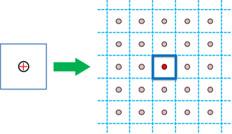
Figure 1: (Color online) Demonstration for the boundary condition of Eq. (17). The influence of the periodic boundary condition can be equivalently replaced by the point “charge” lattice in free space, which is similar like the method of image charges.

Permanent dipole: We first look at the interaction of permanent dipoles $\hat{H}_{12}^{xy}=\xi^{xy}\hat{\tau}_{1}^{x}\hat{\tau}_{2}^{y}$ ($x,y=\mathsf{e},\mathsf{g}$). After the time integration as above, the interaction strength $\xi^{xy}$ is given by ($\mathbf{r}:=\mathbf{x}_{2}-\mathbf{x}_{1}$)

$$\xi^{xy} =\sum_{\mathbf{k},\sigma}-\frac{(g_{1,\mathbf{k}\sigma}^{x})^{*}g_{2,\mathbf{k}\sigma}^{y}}{\hbar\omega_{\mathbf{k}}}+\mathbf{h.c.}$$ (14)

$$= \sum_{\mathbf{k}\neq 0}-\frac{\mu_{0}}{2V}\Big{[}\vec{m}_{1}^{x}\cdot\vec{m}_{2}^{y}+(\vec{m}_{1}^{x}\cdot\nabla_{\mathbf{r}})(\vec{m}_{2}^{y}\cdot\nabla_{\mathbf{r}})\frac{1}{\mathbf{k}^{2}}\Big{]}e^{i\mathbf{k}\cdot\mathbf{r}}+\mathbf{h.c.}$$

Utilizing the normalization relation of $e^{i\mathbf{k}\cdot\mathbf{r}}$ inside the periodic box , the first term in the above summation leads to

$$-\mu_{0}\vec{m}_{1}^{x}\cdot\vec{m}_{2}^{y}\big{[}\sum_{\mathbf{k}\neq 0}\frac{e^{i\mathbf{k}\cdot\mathbf{r}}}{V}\big{]}=\frac{\mu_{0}}{V}\vec{m}_{1}^{x}\cdot\vec{m}_{2}^{y}\big{[}1-V\delta^{(3)}(\mathbf{r})\big{]}.$$ (15)

The second summation term can be calculated by $-\mu_{0}(\vec{m}_{1}^{x}\cdot\nabla_{\mathbf{r}})(\vec{m}_{2}^{y}\cdot\nabla_{\mathbf{r}})\chi_{\text{{p}}}(\mathbf{r})$, where

$$\chi_{\text{{p}}}(\mathbf{r})=\sum_{\mathbf{k}\neq 0}\frac{1}{\mathbf{k}^{2}}\frac{e^{i\mathbf{k}\cdot\mathbf{r}}}{V}$$ (16)

is a generation function. For a finite volume, the field modes are discrete, still the summation in $\chi_{\text{{p}}}(\mathbf{r})$ cannot be turned into integral. Notice that the generation function $\chi_{\text{{p}}}(\mathbf{r})$ is a periodic function $\chi_{\text{{p}}}(\mathbf{r})=\chi_{\text{{p}}}(\mathbf{r}+\mathbf{r}_{\mathbf{n}})$, where $\mathbf{r}_{\mathbf{n}}:=L(n_{x},n_{y},n_{z})$ is a periodicity vector ($n_{i}$ are integers), and it satisfies the following differential equation

$$\nabla^{2}\chi_{\text{{p}}}(\mathbf{r})=-\sum_{\mathbf{k}\neq 0}\frac{e^{i\mathbf{k}\cdot\mathbf{r}}}{V}=-\sum_{\mathbf{n}}\delta^{(3)}(\mathbf{r}-\mathbf{r}_{\mathbf{n}})+\frac{1}{V}.$$ (17)

Here $\chi_{\text{{p}}}(\mathbf{r})$ can be regarded as an “electric potential” in free space, with $-\sum\delta^{(3)}(\mathbf{r}-\mathbf{r}_{n})$ as negative “charges” at $\mathbf{r}_{\mathbf{n}}$, and $1/V$ as a homogenous positive “background” (Fig. 1). Thus, the solution of the above equation is

$$\chi_{\text{{p}}}(\mathbf{r})=\sum_{\mathbf{n}}\frac{1}{4\pi}\frac{-1}{\left|\mathbf{r}-\mathbf{r}_{\mathbf{n}}\right|}+\frac{\mathbf{r}^{2}}{2V}.$$ (18)

Therefore, the permanent dipole interaction strength is

$$\xi^{xy} =\frac{\mu_{0}\,\vec{m}_{1}^{x}\cdot\vec{m}_{2}^{y}}{V}-\mu_{0}(\vec{m}_{1}^{x}\cdot\nabla_{\mathbf{r}})(\vec{m}_{2}^{y}\cdot\nabla_{\mathbf{r}})\chi_{\text{{p}}}(\mathbf{r})$$ (19)

$$=\frac{\mu_{0}}{4\pi}\sum_{\mathbf{n}}\frac{\vec{m}_{1}^{x}\cdot\vec{m}_{2}^{y}-3(\vec{m}_{1}^{x}\cdot\hat{\mathrm{e}}_{\delta\mathbf{r}_{\mathbf{n}}})(\vec{m}_{2}^{y}\cdot\hat{\mathrm{e}}_{\delta\mathbf{r}_{\mathbf{n}}})}{|\Delta\mathbf{r}_{\mathbf{n}}|^{3}},$$

where $\Delta\mathbf{r}_{\mathbf{n}}:=\mathbf{r}-\mathbf{r}_{\mathbf{n}}$, and $\hat{\mathrm{e}}_{\delta\mathbf{r}_{\mathbf{n}}}:=\Delta\mathbf{r}_{\mathbf{n}}/|\Delta\mathbf{r}_{\mathbf{n}}|$.

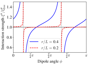
Figure 2: (Color online) Numerical estimation for the dipole-dipole interaction strength in a finite volume [Eq. (19)] comparing with the free space result. Here as an example, we choose $\hat{\mathrm{e}}_{\mathbf{r}}=(1,2,3)/\sqrt{14}$, and set the two dipoles parallel to each other in the direction $\hat{\mathrm{e}}_{1,2}=(\cos\phi,0,\sin\phi)$. When $r/L$ is large, the correction from the boundary effect is significant. It turns out Eq. (19) converges quite fast, and only very few “image” terms is needed ($|n_{x,y,z}|\lesssim 2$) to get a precise enough result, which means only the nearest “image” dipoles are important.

The above result $\xi^{xy}$ only depends on the relative distance $\mathbf{r}=\mathbf{x}_{2}-\mathbf{x}_{1}$, but does not depend the absolute positions $\mathbf{x}_{1,2}$. This is because the box with periodic boundary condition is translationally symmetric, thus every point can be regarded as the box center. Without generality, we set the position of dipole-1 ($\mathbf{x}_{1}$) as the origin, then the position of dipole-2 is $\mathbf{x}_{2}=\mathbf{r}$.

Notice that, the 0-th term [$\mathbf{n}=(0,0,0)$] in the above summation is exactly the same with the free space result Eq. (12). The other summation terms can be regarded as contributions from “image” dipoles of dipole-2 at the positions $\mathbf{r}-\mathbf{r}_{\mathbf{n}}$ reflecting the boundary effect, and they are of order $\sim V^{-1}$. Thus, when $V\rightarrow\infty$, this result returns to the previous free space case.

Fig. 2 shows a numerical estimation for this permanent dipole interaction strength in a finite volume [Eq. (19)] comparing with the free space result [Eq. (12)]. In a finite volume, the dipole-dipole interaction strength can be either enhanced ($\xi^{xy}/\xi_{\mathrm{free}}^{xy}>1$) or decreased ($\xi^{xy}/\xi_{\mathrm{free}}^{xy}<1$), depending on the dipole orientations. There are two diverging points shown in the figure (dashed gray line), this is because around these dipole orientations, $\vec{m}_{1}^{x}\cdot\vec{m}_{2}^{y}-3(\vec{m}_{1}^{x}\cdot\hat{\mathrm{e}}_{\mathbf{r}})(\vec{m}_{2}^{y}\cdot\hat{\mathrm{e}}_{\mathbf{r}})\simeq 0$, thus the free space result approaches zero, which makes $\xi^{xy}/\xi_{\mathrm{free}}^{xy}$ diverge.

If both the two dipoles are placed far away from the boundary, we have $r/L\ll 1$, thus only the 0-th term is important, and that means the dipole interaction is almost the same with free space case. On the other hand, if they are close to the boundary, effectively they get close to the “image” dipoles, thus the correction from the boundary effect becomes significant. This is also quite similar with the situation in classical electrodynamics.

Transition dipole: Now we consider the interaction between two transition dipoles. The interaction strength is

$$\xi^{\text{{t}}} =\sum_{\mathbf{k},\sigma}-\frac{(g_{1,\mathbf{k}\sigma}^{\text{{t}}})^{*}g_{2,\mathbf{k}\sigma}^{\text{{t}}}}{\hbar\omega_{\mathbf{k}}}[1+\frac{\Omega}{\omega_{\mathbf{k}}-\Omega}]+\mathbf{h.c.}$$ (20)

$$=\xi_{0}^{\text{{t}}}+\frac{\mu_{0}\,\vec{m}_{1}^{\text{{t}}}\cdot\vec{m}_{2}^{\text{{t}}}}{V}-\mu_{0}(\vec{m}_{1}^{\text{{t}}}\cdot\nabla_{\mathbf{r}})(\vec{m}_{2}^{\text{{t}}}\cdot\nabla_{\mathbf{r}})\chi_{\text{{t}}}(\mathbf{r}).$$

Here $\xi_{0}^{\text{{t}}}$ has the same form with the permanent dipole interaction Eq. (19), except the dipole index should be changed to “t”, and $\chi_{\text{{t}}}$ is a generation function:

$$\chi_{\text{{t}}}(\mathbf{r}):=\sum_{\mathbf{k}\neq 0}\frac{\Omega}{\omega_{\mathbf{k}}-\Omega}\cdot\frac{e^{i\mathbf{k}\cdot\mathbf{r}}}{\mathbf{k}^{2}}\cdot\frac{1}{V}.$$ (21)

Comparing with the generation function $\chi_{\text{{p}}}$ in the permanent dipoles case, here $\chi_{\text{{t}}}$ contains a sharp envelop $\Omega/(\omega_{\mathbf{k}}-\Omega)$ in the summation. Therefore, only the nearly resonant terms with $\omega_{\mathbf{k}}\simeq\Omega$ contribute significantly in the summation, and they could even dominate over $\xi_{0}^{\text{{t}}}$. Thus, the interaction strength can be also approximately recalculated by

$$\xi^{\text{{t}}}=\sum_{\mathbf{k}}^{\omega_{\mathbf{k}}\simeq\Omega}-\frac{(g_{1,\mathbf{k}\sigma}^{\text{{t}}})^{*}g_{2,\mathbf{k}\sigma}^{\text{{t}}}}{\hbar(\omega_{\mathbf{k}}-\Omega)}+\mathbf{h.c.}$$ (22)

Notice that this result also has a similar form with some previous studies based on adiabatic elimination ($2|g|^{2}/\Delta$) Lambert et al. (2016). Thus, the correction mechanism to the transition dipole interaction in a finite volume is quite similar with the Purcell effect Purcell et al. (1946); Baranov et al. (2016).

V Summary

In this paper, we derived the indirect interaction between two magnetic dipoles induced by the quantized EM field for both free space and finite volume case. A retarded interaction is obtained, and it reduces to a time-local one after RWA and Markovian approximation.

Our result showed that the permanent and transition dipoles should be treated separately. In free space, the interaction between the permanent dipoles directly returns to the classical interaction; the interaction between transition dipoles has the same form with the previous studies on electric dipole interaction, and it does not return to the classical result directly, yet returns in the short-distance limit $r/\lambda\ll 1$.

In a finite volume, both the permanent and transition dipole-dipole interactions are changed, but by different mechanisms. For transition dipoles, this changing mechanism is similar with the Purcell effect, since only a few number of nearly resonant modes take effect in the interaction mediation; for permanent dipoles, still all the field modes take effect for the interaction mediation, but the correction comes from the boundary effect: if the dipoles are placed close to the boundary, the influence is strong, if they are both placed far away from the boundary, their interaction does not change too much from the free space case.

Acknowledgement - This study is supported by Office of Naval Research (Award No. N00014-16-1-3054) and Robert A. Welch Foundation (Grant No. A-1261). S.-W. Li is very grateful for the helpful discussions with Z. Yi at Texas A&M University.

Appendix A The interaction between a magnetic dipole and the EM field

Here we derive the interaction between a magnetic dipole and the EM field. We start from the Hamiltonian of a single atom coupled with the EM field

$$\hat{H}_{S} =\frac{[\hat{\mathbf{p}}-e\hat{\mathbf{A}}(\hat{\mathbf{x}})]^{2}}{2m}+\varphi(\hat{\mathbf{x}}-\mathbf{x}_{0}),$$

$$\hat{H}_{\text{{em}}} =\int dV\,\frac{1}{2}[\epsilon_{0}\mathbf{E}^{2}+\frac{1}{\mu_{0}}\,\mathbf{B}^{2}]=\sum_{\mathbf{k},\sigma}\frac{1}{2}\hbar\omega_{\mathbf{k}}(\hat{a}_{\mathbf{k}\sigma}^{\dagger}\hat{a}_{\mathbf{k}\sigma}+\hat{a}_{\mathbf{k}\sigma}\hat{a}_{\mathbf{k}\sigma}^{\dagger}).$$ (23)

Here $\varphi(\mathbf{x})$ is the electric potential, and $\hat{\mathbf{A}}(\mathbf{x})$ is the field operator

$$\hat{\mathbf{A}}(\mathbf{x})=\sum_{\mathbf{k},\sigma}\hat{\mathrm{e}}_{\mathbf{k}\sigma}\overline{N}_{k}(\hat{a}_{\mathbf{k}\sigma}e^{i\mathbf{k}\cdot\mathbf{x}}+\hat{a}_{\mathbf{k}\sigma}^{\dagger}e^{-i\mathbf{k}\cdot\mathbf{x}}),\qquad\overline{N}_{k}:=\sqrt{\frac{\hbar}{2\epsilon_{0}\omega_{\mathbf{k}}V}}.$$ (24)

We omit the $\hat{\mathbf{A}}^{2}$ term in $\hat{H}_{S}$, and expand $\hat{\mathbf{A}}(\hat{\mathbf{x}})$ around the nucleus position $\mathbf{x}_{0}$ by $e^{i\mathbf{k}\cdot\hat{\mathbf{x}}}\simeq e^{i\mathbf{k}\cdot\mathbf{x}_{0}}\big{[}1+i\mathbf{k}\cdot\hat{\mathbf{r}}+\dots\big{]}$, where $\hat{\mathbf{r}}:=\hat{\mathbf{x}}-\mathbf{x}_{0}$. The zeroth order just gives the interaction of dipole approximation, $\hat{H}_{\mathrm{int}}^{(0)}=-\frac{e}{m}\hat{\mathbf{p}}\cdot\hat{\mathbf{A}}(\mathbf{x}_{0})$ Weinberg (2012).

Now we consider the 1st order in the expansion, which gives

$$\hat{H}_{\mathrm{int}}^{(1)}=\sum_{\mathbf{k},\sigma}-\frac{e}{m}\cdot\overline{N}_{k}(\hat{\mathbf{p}}\cdot\hat{\mathrm{e}}_{\mathbf{k}\sigma})(i\mathbf{k}\cdot\hat{\mathbf{r}})\,(\hat{a}_{\mathbf{k}\sigma}e^{i\mathbf{k}\cdot\mathbf{x}_{0}}-\hat{a}_{\mathbf{k}\sigma}^{\dagger}e^{-i\mathbf{k}\cdot\mathbf{x}_{0}}).$$ (25)

With the help of the relation (denoting $\hat{\mathbf{L}}:=\hat{\mathbf{r}}\times\hat{\mathbf{p}}$)

$$(\hat{\mathbf{p}}\cdot\hat{\mathrm{e}}_{\mathbf{k}\sigma})(i\mathbf{k}\cdot\hat{\mathbf{r}}) =(\hat{\mathbf{p}}\cdot i\mathbf{k})(\hat{\mathbf{r}}\cdot\hat{\mathrm{e}}_{\mathbf{k}\sigma})+(\hat{\mathbf{r}}\times\hat{\mathbf{p}})\cdot(i\mathbf{k}\times\hat{\mathrm{e}}_{\mathbf{k}\sigma})$$

$$=\frac{i|\mathbf{k}|}{2}[(\hat{\mathbf{p}}\cdot\hat{\mathrm{e}}_{\mathbf{k}\sigma})(\hat{\mathbf{r}}\cdot\hat{\mathrm{e}}_{\mathbf{k}})+(\hat{\mathbf{p}}\cdot\hat{\mathrm{e}}_{\mathbf{k}})(\hat{\mathbf{r}}\cdot\hat{\mathrm{e}}_{\mathbf{k}\sigma})]+\frac{1}{2}\hat{\mathbf{L}}\cdot(i\mathbf{k}\times\hat{\mathrm{e}}_{\mathbf{k}\sigma}),$$ (26)

the above interaction Hamiltonian can be written into two terms $\hat{H}_{\mathrm{int}}^{(1)}=\hat{H}_{\mathrm{md}}+\hat{H}_{\mathrm{eq}}$, where $\hat{H}_{\mathrm{md}}$ is the interaction between the magnetic dipole and the EM field (denoting $\hat{\boldsymbol{\mathfrak{m}}}_{L}:=\frac{e}{2m}\hat{\mathbf{L}}$)

$$\hat{H}_{\mathrm{md}}=\sum_{\mathbf{k},\sigma}-\frac{e}{2m}\,\hat{\mathbf{L}}\cdot(i\mathbf{k})\times\hat{\mathrm{e}}_{\mathbf{k}\sigma}\,\overline{N}_{k}(\hat{a}_{\mathbf{k}\sigma}e^{i\mathbf{k}\cdot\mathbf{x}_{0}}-\hat{a}_{\mathbf{k}\sigma}^{\dagger}e^{-i\mathbf{k}\cdot\mathbf{x}_{0}})=-\frac{e}{2m}\hat{\mathbf{L}}\cdot\nabla_{\mathbf{x}_{0}}\times\hat{\mathbf{A}}(\mathbf{x}_{0})=-\hat{\boldsymbol{\mathfrak{m}}}_{L}\cdot\hat{\mathbf{B}}(\mathbf{x}_{0}),$$ (27)

and $\hat{H}_{\mathrm{eq}}$ gives the electric quadrupole interaction (denoting $\hat{p}_{i}=\hat{\mathbf{p}}\cdot\hat{\mathrm{e}}_{i}$, $\hat{r}_{i}=\hat{\mathbf{r}}\cdot\hat{\mathrm{e}}_{i}$) Weinberg (2012)

$$\hat{H}_{\mathrm{eq}} =\sum_{\mathbf{k},\sigma}-\frac{i|\mathbf{k}|e}{2m}\,\big{(}\hat{p}_{\mathbf{k}}\hat{r}_{\sigma}+\hat{p}_{\sigma}\hat{r}_{\mathbf{k}}\big{)}\,\overline{N}_{k}(\hat{a}_{\mathbf{k}\sigma}e^{i\mathbf{k}\cdot\mathbf{x}_{0}}-\hat{a}_{\mathbf{k}\sigma}^{\dagger}e^{-i\mathbf{k}\cdot\mathbf{x}_{0}}).$$ (28)

Appendix B Coupling spectral density in free space

Here we show the derivation of the coupling spectral density $J_{12}^{\mu\nu}(\omega)$ in free space, which is define by

$$J_{12}^{\mu\nu}(\omega)=2\pi\sum_{\mathbf{k}\sigma}(g_{1,\mathbf{k}\sigma}^{\mu})^{*}g_{2,\mathbf{k}\sigma}^{\nu}\delta(\omega-\omega_{\mathbf{k}}),\qquad g_{i,\mathbf{k}\sigma}^{\mu}=-i\vec{m}_{i}^{\mu}\cdot(\hat{\mathrm{e}}_{\mathbf{k}}\times\hat{\mathrm{e}}_{\mathbf{k}\sigma})e^{i\mathbf{k}\cdot\mathbf{x}_{i}}\sqrt{\frac{\mu_{0}\hbar\omega_{k}}{2V}}.$$ (29)

Since the index $\mu$ only appears on $\vec{m}_{i}^{\mu}$ in $J_{12}^{\mu\nu}(\omega)$ to represent the transition/permanent dipole, hereafter we omit it for simplicity.

The summation over $\mathbf{k},\sigma$ is changed into integral by

$$\sum_{\mathbf{k},\sigma}[...]\quad\longrightarrow\quad\sum_{\sigma}\frac{V}{(2\pi)^{3}}\int d^{3}\mathbf{k}\,[...]=\sum_{\sigma}\frac{V}{(2\pi c)^{3}}\int\omega^{2}d\omega\int d\Omega\,[...]$$ (30)

Thus the coupling spectral density $J_{12}(\omega)$ is given by (denoting $\mathbf{r}:=\mathbf{x}_{2}-\mathbf{x}_{1}$)

$$J_{12}(\omega) =\frac{2\pi}{(2\pi c)^{3}}\,\frac{\mu_{0}\hbar\omega^{3}}{2}\int_{0}^{2\pi}d\varphi\int_{0}^{\pi}\sin\theta d\theta\,e^{i\mathbf{k}\cdot(\mathbf{x}_{2}-\mathbf{x}_{1})}\sum_{\sigma}[\vec{m}_{1}\cdot(\hat{\mathrm{e}}_{\mathbf{k}}\times\hat{\mathrm{e}}_{\mathbf{k}\sigma})][\vec{m}_{2}\cdot(\hat{\mathrm{e}}_{\mathbf{k}}\times\hat{\mathrm{e}}_{\mathbf{k}\sigma})]$$

$$=\frac{1}{(2\pi)^{2}c^{3}}\,\frac{\mu_{0}\hbar\omega^{3}}{2}\int_{0}^{2\pi}d\varphi\int_{0}^{\pi}\sin\theta d\theta\,e^{i\mathbf{k}\cdot\mathbf{r}}\Big{[}\vec{m}_{1}\cdot\vec{m}_{2}-(\vec{m}_{1}\cdot\hat{\mathrm{e}}_{\mathbf{k}})(\vec{m}_{2}\cdot\hat{\mathrm{e}}_{\mathbf{k}})\Big{]}.$$ (31)

To calculate the above integral, we use the vector $\mathbf{r}$ and $\vec{m}_{1}$ to span a proper coordinate. We set $\hat{\mathrm{e}}_{z}:=\mathbf{r}/r:=\hat{\mathrm{e}}_{\mathbf{r}}$, and $\hat{\mathrm{e}}_{y}:=\lambda^{\text{-}1}\mathbf{r}\times\vec{m}_{1}$, where $\lambda=\sqrt{r^{2}\vec{m}_{1}^{2}+(\mathbf{r}\cdot\vec{m}_{1})^{2}}$ is a normalization factor, and $r:=|\mathbf{r}|$; then we have $\hat{\mathrm{e}}_{x}=\hat{\mathrm{e}}_{y}\times\hat{\mathrm{e}}_{z}=\lambda^{\text{-}1}[r\vec{m}_{1}-(\mathbf{r}\cdot\vec{m}_{1})\mathbf{r}/r]$.

With this basis $\hat{\mathrm{e}}_{x,y,z}$, the vectors in the above integral can be written as

$$\hat{\mathrm{e}}_{\mathbf{k}} =\sin\theta\cos\varphi\,\hat{\mathrm{e}}_{x}+\sin\theta\sin\varphi\,\hat{\mathrm{e}}_{y}+\cos\theta\,\hat{\mathrm{e}}_{z},$$

$$\vec{m}_{1} =\frac{\lambda}{r}\hat{\mathrm{e}}_{x}+(\vec{m}_{1}\cdot\hat{\mathrm{e}}_{\mathbf{r}})\hat{\mathrm{e}}_{z},$$ (32)

$$\vec{m}_{2} =\sum_{i}(\vec{m}_{2}\cdot\hat{\mathrm{e}}_{i})\hat{\mathrm{e}}_{i}=\frac{r}{\lambda}[\vec{m}_{2}\cdot\vec{m}_{1}-(\vec{m}_{1}\cdot\hat{\mathrm{e}}_{\mathbf{r}})(\vec{m}_{2}\cdot\hat{\mathrm{e}}_{\mathbf{r}})]\hat{\mathrm{e}}_{x}+\frac{r}{\lambda}(\hat{\mathrm{e}}_{\mathbf{r}}\cdot\vec{m}_{1}\times\vec{m}_{2})\hat{\mathrm{e}}_{y}+(\vec{m}_{2}\cdot\hat{\mathrm{e}}_{\mathbf{r}})\hat{\mathrm{e}}_{z}.$$

Thus the products in the integral give

$$\vec{m}_{1}\cdot\hat{\mathrm{e}}_{\mathbf{k}}= \frac{\lambda}{r}\sin\theta\cos\varphi+(\vec{m}_{1}\cdot\hat{\mathrm{e}}_{\mathbf{r}})\cos\theta,$$

$$\vec{m}_{2}\cdot\hat{\mathrm{e}}_{\mathbf{k}}= \frac{r}{\lambda}(\vec{m}_{1}\times\hat{\mathrm{e}}_{\mathbf{r}})\cdot(\vec{m}_{2}\times\hat{\mathrm{e}}_{\mathbf{r}})\sin\theta\cos\varphi+\frac{r}{\lambda}(\hat{\mathrm{e}}_{\mathbf{r}}\cdot\vec{m}_{1}\times\vec{m}_{2})\sin\theta\sin\varphi+(\vec{m}_{2}\cdot\hat{\mathrm{e}}_{\mathbf{r}})\cos\theta.$$ (33)

In the product $(\vec{m}_{1}\cdot\hat{\mathrm{e}}_{\mathbf{k}})(\vec{m}_{2}\cdot\hat{\mathrm{e}}_{\mathbf{k}})$, if we first integrate over $\varphi\in[0,2\pi]$, it turns out that most terms vanish directly, and the remaining terms are

$$\mathbf{I}_{0} =\int_{0}^{2\pi}d\varphi\int_{0}^{\pi}\sin\theta d\theta\,e^{ikr\cos\theta}\vec{m}_{2}\cdot\vec{m}_{1}=4\pi\vec{m}_{2}\cdot\vec{m}_{1}\,\frac{\sin kr}{kr},$$

$$\mathbf{I}_{1} =\int_{0}^{2\pi}d\varphi\int_{0}^{\pi}\sin\theta d\theta\,e^{ikr\cos\theta}(\vec{m}_{1}\times\hat{\mathrm{e}}_{\mathbf{r}})\cdot(\vec{m}_{2}\times\hat{\mathrm{e}}_{\mathbf{r}})\sin^{2}\theta\cos^{2}\varphi=4\pi(\vec{m}_{1}\times\hat{\mathrm{e}}_{\mathbf{r}})\cdot(\vec{m}_{2}\times\hat{\mathrm{e}}_{\mathbf{r}})\big{[}\frac{\sin kr}{(kr)^{3}}-\frac{\cos kr}{(kr)^{2}}\big{]},$$

$$\mathbf{I}_{2} =\int_{0}^{2\pi}d\varphi\int_{0}^{\pi}\sin\theta d\theta\,e^{ikr\cos\theta}(\hat{m}_{1}\cdot\hat{\mathrm{e}}_{\mathbf{r}})(\hat{m}_{2}\cdot\hat{\mathrm{e}}_{\mathbf{r}})\cos^{2}\theta=4\pi(\vec{m}_{1}\cdot\hat{\mathrm{e}}_{\mathbf{r}})(\vec{m}_{2}\cdot\hat{\mathrm{e}}_{\mathbf{r}})\big{[}\frac{\sin kr}{kr}+\frac{2\cos kr}{(kr)^{2}}-\frac{2\sin kr}{(kr)^{3}}\big{]}.$$ (34)

Therefore, we have

$$J_{12}(\omega=ck)= \frac{\mu_{0}\hbar k^{3}}{2\pi}\Big{\{}\vec{m}_{1}\cdot\vec{m}_{2}\frac{\sin kr}{kr}-(\vec{m}_{1}\times\hat{\mathrm{e}}_{\mathbf{r}})\cdot(\vec{m}_{2}\times\hat{\mathrm{e}}_{\mathbf{r}})\big{[}\frac{\sin kr}{(kr)^{3}}-\frac{\cos kr}{(kr)^{2}}\big{]}$$

$$-(\vec{m}_{1}\cdot\hat{\mathrm{e}}_{\mathbf{r}})(\vec{m}_{2}\cdot\hat{\mathrm{e}}_{\mathbf{r}})\,\big{[}\frac{\sin kr}{kr}+\frac{2\cos kr}{(kr)^{2}}-\frac{2\sin kr}{(kr)^{3}}\big{]}\Big{\}}.$$ (35)

which is an odd function $J_{12}(-\omega)=-J_{12}(\omega)$, and we also have $J_{12}(\omega)=J_{21}(\omega)$.

Notice that, using this coupling spectral density (proper indices for $\text{{t}},\mathsf{e},\mathsf{g}$ should be added to $\vec{m}_{i}$), the interaction strength of the permanent dipoles is

$$\xi^{\text{{p}}}=-\int_{-\infty}^{\infty}\frac{d\omega}{2\pi\hbar}\,\frac{J_{12}(\omega)}{\omega} =\frac{\mu_{0}}{r^{3}}\int_{-\infty}^{\infty}\frac{d(kr)}{2\pi}\,\frac{1}{kr}\cdot\frac{(kr)^{3}}{2\pi}\Big{\{}(\vec{m}_{1}\times\hat{\mathrm{e}}_{\mathbf{r}})\cdot(\vec{m}_{2}\times\hat{\mathrm{e}}_{\mathbf{r}})-2(\vec{m}_{1}\cdot\hat{\mathrm{e}}_{\mathbf{r}})(\vec{m}_{2}\cdot\hat{\mathrm{e}}_{\mathbf{r}})\Big{\}}\frac{\sin kr}{(kr)^{3}}$$

$$=\frac{\mu_{0}}{4\pi r^{3}}\big{[}\vec{m}_{1}\cdot\vec{m}_{2}-3(\vec{m}_{1}\cdot\hat{\mathrm{e}}_{\mathbf{r}})(\vec{m}_{2}\cdot\hat{\mathrm{e}}_{\mathbf{r}})\big{]},$$ (36)

which has exactly the same form with the classical dipole-dipole interaction.

On the other hand, the interaction strength between the transition dipoles is given by

$$\xi^{\text{{t}}}=-\int_{-\infty}^{\infty}\frac{d\omega}{2\pi\hbar}\,\frac{J_{12}(\omega)}{\omega-\Omega}= -\frac{\mu_{0}}{4\pi r^{3}}\int_{-\infty}^{\infty}\frac{dx}{\pi}\,\frac{x^{3}}{x-x_{\Omega}}\Big{\{}\vec{m}_{1}\cdot\vec{m}_{2}\frac{\sin x}{x}-(\vec{m}_{1}\times\hat{\mathrm{e}}_{\mathbf{r}})\cdot(\vec{m}_{2}\times\hat{\mathrm{e}}_{\mathbf{r}})\big{[}\frac{\sin x}{x^{3}}-\frac{\cos x}{x^{2}}\big{]}$$

$$\qquad-(\vec{m}_{1}\cdot\hat{\mathrm{e}}_{\mathbf{r}})(\vec{m}_{2}\cdot\hat{\mathrm{e}}_{\mathbf{r}})\,\big{[}\frac{\sin x}{x}+\frac{2\cos x}{x^{2}}-\frac{2\sin x}{x^{3}}\big{]}\Big{\}}$$

$$= -\frac{\mu_{0}}{4\pi r^{3}}\Big{\{}\vec{m}_{1}\cdot\vec{m}_{2}x_{\Omega}^{2}\cos x_{\Omega}-(\vec{m}_{1}\times\hat{\mathrm{e}}_{\mathbf{r}})\cdot(\vec{m}_{2}\times\hat{\mathrm{e}}_{\mathbf{r}})\big{[}\cos x_{\Omega}-x_{\Omega}\sin x_{\Omega}\big{]}$$

$$\qquad-(\vec{m}_{1}\cdot\hat{\mathrm{e}}_{\mathbf{r}})(\vec{m}_{2}\cdot\hat{\mathrm{e}}_{\mathbf{r}})\,\big{[}2x_{\Omega}\sin x_{\Omega}+x_{\Omega}^{2}\cos x_{\Omega}-2\cos x_{\Omega}\big{]}\Big{\}},$$ (37)

where $x_{\Omega}:=r\Omega/c=2\pi r/\lambda$, and $\lambda$ is the wavelength corresponding to the transition frequency $\Omega$. In the short-distance limit $x_{\Omega}\rightarrow 0$, the above interaction strength $\xi^{\text{{t}}}$ returns to the same form as $\xi^{\text{{p}}}$ [Eq. (36)], which is just the classical result.

References

• Liao and Zubairy (2014) Z. Liao and M. S. Zubairy, Phys. Rev. A 90, 053805 (2014).
• Liao et al. (2015) Z. Liao, X. Zeng, S.-Y. Zhu,  and M. S. Zubairy, Phys. Rev. A 92, 023806 (2015).
• Lambert et al. (2016) N. J. Lambert, J. A. Haigh, S. Langenfeld, A. C. Doherty,  and A. J. Ferguson, Phys. Rev. A 93, 021803 (2016).
• Baranov et al. (2016) D. G. Baranov, R. S. Savelev, S. V. Li, A. E. Krasnok,  and A. Alù, arXiv:1610.02001  (2016).
• Liao et al. (2016) Z. Liao, H. Nha,  and M. S. Zubairy, Phys. Rev. A 94, 053842 (2016).
• Shahmoon and Kurizki (2013a) E. Shahmoon and G. Kurizki, Phys. Rev. A 87, 033831 (2013a).
• Shahmoon and Kurizki (2013b) E. Shahmoon and G. Kurizki, Phys. Rev. A 87, 062105 (2013b).
• Cai et al. (2016) H. Cai, D.-W. Wang, A. A. Svidzinsky, S.-Y. Zhu,  and M. O. Scully, Phys. Rev. A 93, 053804 (2016).
• Shahmoon (2017) E. Shahmoon, Phys. Rev. A 95, 062504 (2017).
• Donaire et al. (2017) M. Donaire, J. M. Muñoz-Castañeda,  and L. M. Nieto, Phys. Rev. A 96, 042714 (2017).
• Cortes and Jacob (2017) C. L. Cortes and Z. Jacob, Nature Comm. 8, 14144 (2017).
• Martinis et al. (2005) J. M. Martinis, K. B. Cooper, R. McDermott, M. Steffen, M. Ansmann, K. D. Osborn, K. Cicak, S. Oh, D. P. Pappas, R. W. Simmonds,  and C. C. Yu, Phys. Rev. Lett. 95, 210503 (2005).
• Paik et al. (2011) H. Paik, D. I. Schuster, L. S. Bishop, G. Kirchmair, G. Catelani, A. P. Sears, B. R. Johnson, M. J. Reagor, L. Frunzio, L. I. Glazman, S. M. Girvin, M. H. Devoret,  and R. J. Schoelkopf, Phys. Rev. Lett. 107, 240501 (2011).
• Rigetti et al. (2012) C. Rigetti, J. M. Gambetta, S. Poletto, B. L. T. Plourde, J. M. Chow, A. D. Córcoles, J. A. Smolin, S. T. Merkel, J. R. Rozen, G. A. Keefe, M. B. Rothwell, M. B. Ketchen,  and M. Steffen, Physical Review B 86, 100506 (2012).
• Lisenfeld et al. (2016) J. Lisenfeld, A. Bilmes, S. Matityahu, S. Zanker, M. Marthaler, M. Schechter, G. Schön, A. Shnirman, G. Weiss,  and A. V. Ustinov, Sci. Rep. 6, srep23786 (2016).
• Doherty et al. (2013) M. W. Doherty, N. B. Manson, P. Delaney, F. Jelezko, J. Wrachtrup,  and L. C. L. Hollenberg, Phys. Rep. 528, 1 (2013).
• Zhao et al. (2012) N. Zhao, S.-W. Ho,  and R.-B. Liu, Phys. Rev. B 85, 115303 (2012).
• Yang et al. (2010) S. Yang, D. Z. Xu, Z. Song,  and C. P. Sun, J. Chem. Phys. 132, 234501 (2010).
• El-Ganainy and John (2013) R. El-Ganainy and S. John, New J. Phys. 15, 083033 (2013).
• Dong et al. (2016) H. Dong, S.-W. Li, Z. Yi, G. S. Agarwal,  and M. O. Scully, arXiv:1608.04364  (2016).
• Jackson (1998) J. D. Jackson, Classical Electrodynamics Third Edition, 3rd ed. (Wiley, New York, 1998).
• Lyuboshitz (1968) V. L. Lyuboshitz, Sov. Phys. JETP 26, 937 (1968).
• Lehmberg (1970) R. H. Lehmberg, Phys. Rev. A 2, 883 (1970).
• Ficek et al. (1987) Z. Ficek, R. Tanaś,  and S. Kielich, Physica A 146, 452 (1987).
• Agarwal (1974) G. S. Agarwal, Quantum statistical theories of spontaneous emission and their relation to other approaches (Springer, 1974).
• Ficek and Swain (2005) Z. Ficek and S. Swain, Quantum Interference and Coherence: Theory and Experiments, 1st ed. (Springer, Berlin, 2005).
• Dicke (1954) R. H. Dicke, Phys. Rev. 93, 99 (1954).
• Cohen-Tannoudji et al. (1989) C. Cohen-Tannoudji, J. Dupont-Roc,  and G. Grynberg, Photons and Atoms: Introduction to Quantum Electrodynamics, 1st ed. (Wiley-VCH, New York, 1989).
• Ryder (1996) L. H. Ryder, Quantum Field Theory, 2nd ed. (Cambridge University Press, Cambridge ; New York, 1996).
• Purcell et al. (1946) E. M. Purcell, H. C. Torrey,  and R. V. Pound, Phys. Rev. 69, 37 (1946).
• Scully and Zubairy (1997) M. O. Scully and M. S. Zubairy, Quantum optics (Cambridge university press, 1997).
• Weinberg (2012) S. Weinberg, Lectures on quantum mechanics (Cambridge University Press, 2012).
• Breuer and Petruccione (2002) H. Breuer and F. Petruccione, The theory of open quantum systems (Oxford University Press, 2002).
• Li et al. (2015) S.-W. Li, C. Y. Cai,  and C. P. Sun, Ann. Phys. 360, 19 (2015), arXiv: 1407.4290.
• Li et al. (2014) S.-W. Li, L.-P. Yang,  and C.-P. Sun, Eur. Phys. J. D 68, 45 (2014), arXiv:1303.1266.
• Gardiner and Zoller (2004) C. Gardiner and P. Zoller, Quantum noise, Vol. 56 (Springer, 2004).
• Li (2017) S.-W. Li, Phys. Rev. E 96, 012139 (2017), arXiv: 1612.03884.