Inf-sup stable finite elements on barycentric refinements producing divergence–free approximations in arbitrary dimensions

Abstract

We construct several stable finite element pairs for the Stokes problem on barycentric refinements in arbitrary dimensions. A key feature of the spaces is that the divergence maps the discrete velocity space onto the the discrete pressure space; thus, when applied to models of incompressible flows, the pairs yield divergence-free velocity approximations. The key result is a local inf-sup stability that holds for any dimension and for any polynomial degree. With this result, we construct global divergence-free and stable pairs in arbitrary dimension and for any polynomial degree.

1 Introduction

In the papers [2, 17] it was shown that $\bm{\EuScript{P}}^{c}_{k}-\EuScript{P}_{k-1}$ is an inf-sup stable and divergence-free pair on barycentric refine meshes in two and three dimensions if the polynomial size $k$ is sufficiently large. The strategy in the analysis, as shown by Zhang [17], is Stenberg’s macro-element technique [16], where the crucial step is a local inf-sup stability estimate on each macro tetrahedra/triangle. Then, Bernardi-Raugel [3] finite elements are implicitly used to control piecewise constants to prove global inf-sup stability. The use of the Bernardi-Raugel finite elements is the reason one needs a restriction on $k$ to ensure global inf-sup stability: For dimension $d=2$, $k\geq 2$ and for dimension $d=3$, $k\geq 3$.

One of our contributions in this paper is to extend the results in [2, 17] to arbitrary space dimension $d\geq 2$. The key step, as in [17], is to prove a local inf-sup stability result. By definition, a barycentric refinement takes a given mesh (which we call the macro mesh) and adds the barycenter of each simplex of the macro mesh to the set of vertices. We slightly generalize this construction by showing that one can use any arbitrary point in the interior of each simplex (not just the barycenter), as long as the resulting mesh is shape regular.

We then derive several applications of the local inf-sup stability result. First, we with the help of the Bernardi-Raugel element, we show that $\bm{\EuScript{P}}^{c}_{k}-\EuScript{P}_{k-1}$ is inf-sup on the refined mesh for $k\geq d$ (as was shown in [2, 17] for $d=2,3$). For lower order approximations $1\leq k<d$, we use an idea introduced in [10] and supplement the velocity space to obtain an inf-sup stable pair. To this end, we construct vector-valued, piecewise polynomial functions with respect to the refined mesh that have the same trace as the Bernardi-Raugel face bubbles on the skeleton of the macro mesh. The key difference, compared to the Bernardi-Raugel face bubbles, is that the divergence of these functions are piecewise constant. The existence of such finite element functions, which we call modified face bubbles, is guaranteed by the local inf-sup stability result. Thus, we supplement $\bm{\EuScript{P}}^{c}_{k}$ (for $1\leq k<d$) locally with these modified face bubbles to get an inf-sup stable pair on the refined mesh.

We also consider finite elements on the (unrefined) macro mesh. We show that $\bm{\EuScript{P}}^{c}_{1}-\EuScript{P}_{0}$ can be made stable by supplementing the velocity space $\bm{\EuScript{P}}^{c}_{1}$ with the modified face bubbles. Since the divergence of the modified face bubbles are piecewise constant, and thus contained in the pressure space, these finite element will produce divergence-free approximations for the Stokes and NSE problems. These finite elements are developed in arbitrary dimension. The two-dimensional case seems to coincide with a pair of finite elements considered in [5].

A final application is inspired by a finite element introduced in [1]. There, an inf-sup stable and divergence-free macro element pair is constructed in two dimensions with a piecewise linear, continuous pressure space. Again, with the help of the modified face bubbles, we extend these results to arbitrary dimension $d\geq 3$.

Advantages of divergence-free pairs for the Stokes/NSE problems include, e.g., better stability and error estimates, and the enforcement of several conservation laws and invariant properties. We refer the reader to the survey article [11] which highlights the benefits of divergence-free pairs. In addition to the above references, several other inf-sup stable pair of spaces that produce divergence-free approximations have been constructed. These include high-order finite elements ($k\geq 2d$) in two and three dimensions [14, 7, 12, 18], as well as lower order pairs supplemented with rational functions [9, 10]. Advantages of the proposed elements given here are its relative simplicity and flexibility with respect to dimension and polynomial degree. The shape functions are piecewise polynomials and therefore quadrature rules are immediately available. We mention that the degrees of freedom of our lowest-order element agree with those given in [5], where divergence-free Stokes elements with respect to Powell-Sabin partitions are considered (e.g., in three dimensions, every tetrahedron is split into $12$ sub-elements). However, our elements are defined on a less stringent barycenter partition, which makes the implementation simpler.

The paper is organized as follows. In the next section we introduce some notation used throughout the paper. Then, in Section 3 a local inf-sup stability result is proved. In Section 4 the Bernardi-Raguel face bubble functions and its modification are introduced. Then in Section 5 a low-order, divergence-free, and inf-sup pair on the macro mesh is constructed. Finally, in Section 6, inf-sup and divergence-free stable finite elements are given on the refined mesh.

2 Notation and Preliminaries

We consider a family of shape regular $\{\mathcal{T}_{h}\}$ conforming simplicial triangulation of a polytope domain $\Omega\subset\mathbb{R}^{d}$. For each $K\in\mathcal{T}_{h}$ let $x_{K}\in K$ be an interior point, and consider the refined triangulation $\mathcal{T}_{h}$ that subdivides each simplex $K$ into $(d+1)$ simplices by adjoining the vertices of $K$ with the new vertex $x_{K}$. The resulting refined triangulation is denoted by $\mathcal{T}_{h}^{r}$. We assume that the point $x_{K}$ are chosen so that the family $\{\mathcal{T}_{h}^{r}\}$ is also shape regular. If $x_{K}$ is the barycenter of $K$, which is the most practical choice, then $\mathcal{T}_{h}^{r}$ is the barycentric refinement of $\mathcal{T}_{h}$. For any simplex $K$ we let $\EuScript{P}_{k}(K)$ be the space of polynomials of degree at most $k$ defined on $K$. The vector-valued polynomials on a simplex are given by $\bm{\EuScript{P}}_{k}(K)=[\EuScript{P}(K)]^{d}$. We define

$$\mathring{\bm{\EuScript{P}}}_{k}^{c}(\mathcal{S}): =\{\bm{v}\in\bm{H}^{1}_{0}(\Omega):\ \bm{v}|_{K}\in\bm{\EuScript{P}}_{k}(K),\ \forall K\in\mathcal{S}\},$$

$$\mathring{\EuScript{P}}_{k}(\mathcal{S}): =\{q\in L^{2}_{0}(\Omega):\ q|_{K}\in\EuScript{P}_{k}(K),\ \forall K\in\mathcal{S}\},$$

with either $\mathcal{S}=\mathcal{T}_{h}$ or $\mathcal{S}=\mathcal{T}_{h}^{r}$.

We denote by $K^{r}$ the triangulation of $K$:

$$K^{r}=\{T\in\mathcal{T}_{h}^{r}:T\subset K\},$$

and will use the notation

$$\mathring{\bm{\EuScript{P}}}_{k}^{c}(K^{r}): =\{\bm{v}\in\bm{H}^{1}_{0}(K):\ \bm{v}|_{T}\in\bm{\EuScript{P}}_{k}(T),\ \forall T\in K^{r}\},$$ (2.1)

$$\mathring{\EuScript{P}}_{k}(K^{r}): =\{q\in L^{2}_{0}(K):\ q|_{T}\in\EuScript{P}_{k}(T),\ \forall T\in K^{r}\}.$$ (2.2)

3 Local inf-sup stability

In this section we will prove that $\mathring{\bm{\EuScript{P}}}_{k}^{c}(K^{r})-{\mathring{\EuScript{P}}_{k-1}(K^{r})}$ is inf-sup stable for each $K\in\mathcal{T}_{h}$. The result can be stated as follows.

Theorem 3.1.

Let $k\geq 1$. For any $K\in\mathcal{T}_{h}$ and for any $p\in\mathring{\EuScript{P}}_{k-1}(K^{r})$, there exists $\bm{v}\in\mathring{\bm{\EuScript{P}}}_{k}^{c}(K^{r})$ such that

$${\mathop{\mathrm{div}\,}}\bm{v}=p\quad\text{ on }K,$$ (3.1)

with the bound

$$\|\bm{v}\|_{H^{1}(K)}\leq C\|p\|_{L^{2}(K)},$$ (3.2)

where the constant $C>0$ only depends on $k$ and the shape regularity of $K^{r}$, but is independent of $p$.

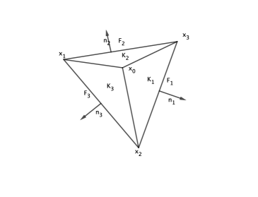
Figure 1: Figure of macro triangle

The proof of Theorem 3.1 will follow from several lemmas. First, we will need some notation. For $K\in\mathcal{T}_{h}$, denote by $S=\{x_{1},\ldots,x_{d+1}\}$ the set of vertices of $K$, and let $x_{0}=x_{K}$. Then the refinement of $K$ is given by $K^{r}=\{K_{i}\}_{1\leq i\leq d+1}$, where $K_{i}$ is the simplex with vertices $\{x_{0}\}\cup S\backslash\{x_{i}\}$. We let $F_{i}$ be the $(d-1)$ dimensional face of $K$ opposite to $x_{i}$, and let $\bm{n}_{i}$ be the unit-normal to $F_{i}$ pointing out of $K$; see Figure 1. In addition to (2.1)–(2.2) we define the polynomial spaces

$$\EuScript{P}_{k}(K^{r}): =\{v\in L^{2}(K):v|_{K_{i}}\in\EuScript{P}_{k}(K_{i}),\ 1\leq i\leq d+1\},\quad \bm{\EuScript{P}}_{k}(K^{r}):=[\EuScript{P}_{k}(K^{r})]^{d},$$

$$\EuScript{P}_{k}^{c}(K^{r}): =\EuScript{P}_{k}(K^{r})\cap H^{1}(K),\quad \bm{\EuScript{P}}_{k}^{c}(K^{r}):=[\EuScript{P}_{k}^{c}(K^{r})]^{d}.$$

Note that $\mathring{\bm{\EuScript{P}}}_{k}^{c}(K^{r})=\bm{\EuScript{P}}_{k}^{c}(K^{r})\cap\bm{H}_{0}^{1}(K)$ and $\mathring{\EuScript{P}}_{k}(K^{r})=\EuScript{P}_{k}(K^{r})\cap L_{0}^{2}(K)$.

For $0\leq i\leq d+1$, we let $\lambda_{i}\in\EuScript{P}_{1}^{c}(K^{r})$ be the continuous, piecewise linear function satisfying $\lambda_{i}(x_{j})=\delta_{ij}$. We note that $\lambda_{i}$ vanishes on $K_{i}$. For a multi-index $\alpha=(\alpha_{1},\alpha_{2},\ldots,\alpha_{d+1})$ we will use the notation

$${\bm{\lambda}}^{\alpha}=\lambda_{1}^{\alpha_{1}}\cdots\lambda_{d+1}^{\alpha_{d+1}}.$$

We note that

$$\nabla({\bm{\lambda}}^{\alpha})=\sum_{j=1}^{d+1}\alpha_{j}{\bm{\lambda}}^{\alpha-e_{j}}\nabla\lambda_{j},$$ (3.3)

where $\{e_{j}\}_{j=1}^{d+1}$ is canonical basis of $\mathbb{R}^{d+1}$. We also define

$$N(\alpha)=\{i:\alpha_{i}>0\}.$$

Hence, ${\bm{\lambda}}^{\alpha}$ vanishes on $K_{i}$ for all $i\in N(\alpha)$.

We let $h_{K}$ be the diameter of $K$, and let $\rho_{K}$ be the diameter of the largest ball inscribed in $K$. The shape regularity constant of $K$ is defined by

$$C_{K}=\frac{h_{K}}{\rho_{K}}.$$

Analogously we let $C_{K_{i}}$ be the shape regularity constant of $K_{i}$ (for $i=1,2\cdots,d+1$), and let $\mathcal{C}_{K}=\max_{1\leq i\leq d+1}C_{K_{i}}$ denote the shape regularity constant of $K^{r}$. We see that $\mathcal{C}_{K}$ is comparable to $C_{K}$ provided $x_{0}$ is sufficiently far from ${\partial}K$.

It is well known that for $0\leq i\leq d+1$, we have

$$\|\nabla\lambda_{i}\|_{L^{\infty}(K)}\leq\frac{C}{h_{K}},$$

where $C$ only depends on $\mathcal{C}_{K}$. Hence, we also have

$$\|\nabla({\bm{\lambda}}^{\alpha})\|_{L^{\infty}(K)}\leq\frac{C}{h_{K}},$$ (3.4)

where $C$ only depends on $\mathcal{C}_{K}$ and $|\alpha|$. In particular, we have

$$\nabla\lambda_{0}|_{K_{i}}=-\frac{1}{h_{i}}\bm{n}_{i},$$ (3.5)

where $h_{i}$ is the distance of $x_{0}$ to the $(d-1)$ dimensional hyperplane that contains $F_{i}$. We note that

$$h_{i}\leq Ch_{K}\text{ for }1\leq i\leq d+1,$$ (3.6)

where $C$ depends only on $\mathcal{C}_{K}$.

Any $d$ unit normals $\{\bm{n}_{i_{1}},\cdots,\bm{n}_{i_{d}}\}$ where $1\leq i_{1}<i_{2}<\cdots<i_{d}\leq d+1$ are linearly independent, and thus span $\mathbb{R}^{d}$. Moreover, the $\ell^{2}$-norm of the inverse of the matrix $A=[\bm{n}_{i_{1}},\bm{n}_{i-2},\cdots,\bm{n}_{i_{d}}]^{t}$ depends on the shape regularity constant of $K$. More precisely, given any $\bm{r}\in\mathbb{R}^{d}$ there exists a unique $\bm{s}\in\mathbb{R}^{d}$ such that

$$A\bm{s}=\bm{r}$$ (3.7)

with

$$|\bm{s}|\leq C|\bm{r}|,$$ (3.8)

where $C$ depends only on $C_{K}$.

We are interested in piecewise polynomials of the form

$$p=\lambda_{0}^{\ell}\sum_{|\alpha|=m}a_{\alpha}{\bm{\lambda}}^{\alpha},\quad a_{\alpha}\in\EuScript{P}_{0}(K^{r}),$$

and $a_{\alpha}|_{K_{i}}=0\text{ for }i\in N(\alpha)$. A scaling argument shows that

$$\sum_{|\alpha|=m}\|a_{\alpha}\|_{L^{2}(K)}^{2}\approx\|p\|_{L^{2}(K)}^{2},$$ (3.9)

where the hidden constants depend on the shape regularity of $K^{r}$, $m$ and $\ell$. In fact, the following decomposition for $\EuScript{P}_{s}(K^{r})$ holds. The result essentially follows from (3.9), so we omit the details.

Lemma 3.2.

Every $p\in\EuScript{P}_{s}(K^{r})$ can be written uniquely as

$$p=\sum_{\ell=0}^{s}p_{\ell},\quad p_{\ell}=\lambda_{0}^{\ell}\sum_{|\alpha|=s-\ell}a_{\alpha}{\bm{\lambda}}^{\alpha},$$ (3.10)

where $a_{\alpha}\in\EuScript{P}_{0}(K^{r})$, and $a_{\alpha}|_{K_{i}}=0\text{ for }i\in N(\alpha)$. Moreover,

$$\sum_{\ell=0}^{s}\|p_{\ell}\|_{L^{2}(K)}^{2}\leq C\|p\|_{L^{2}(K)}^{2},$$

where the constant $C$ depends on the shape regularity constant of $K^{r}$ and $s$.

As mentioned earlier, we will prove Theorem 3.1 in several steps. First, we establish the following lemma.

Lemma 3.3.

Let $p=\lambda_{0}^{\ell}\sum_{|\alpha|=m}b_{\alpha}{\bm{\lambda}}^{\alpha}$ with $m\geq 1$, $b_{\alpha}\in\EuScript{P}_{0}(K^{r})$, with $b_{\alpha}|_{K_{i}}=0$ for all $i\in N(\alpha)$. Then there exists $\bm{v}\in\mathring{\bm{\EuScript{P}}}_{\ell+m+1}^{c}(K^{r})$ such that

$${\mathop{\mathrm{div}\,}}\bm{v}=p+q\text{ on }K,$$ (3.11)

where $q$ is of the form $q=\lambda_{0}^{\ell+1}\sum_{|\alpha|=m-1}c_{\alpha}{\bm{\lambda}}^{\alpha}$ with $c_{\alpha}\in\EuScript{P}_{0}(K^{r})$, with $c_{\alpha}|_{K_{i}}=0$ for all $i\in N(\alpha)$. Moreover, the following bounds hold

$$\|\bm{v}\|_{H^{1}(K)}\leq C\|p\|_{L^{2}(K)},\qquad\|q\|_{L^{2}(K)}\leq C\|p\|_{L^{2}(K)}.$$ (3.12)

Proof.

Since $|\alpha|=m\geq 1$, the set $\{i:i\notin N(\alpha)\}$ has at most $d$ elements. Using the relation (3.5), solvability of (3.7), and the estimates (3.6), (3.8), we conclude that there exists $\bm{s}_{\alpha}\in\mathbb{R}^{d}$ such that

$$(\ell+1)\bm{s}_{\alpha}\cdot\nabla\lambda_{0}|_{K_{i}}=b_{\alpha}|_{K_{i}}\text{ for all }i\notin N(\alpha),$$

with the bound

$$|\bm{s}_{\alpha}|\leq Ch_{K}\|b_{\alpha}\|_{L^{\infty}(K)},$$ (3.13)

where the constant $C$ depends on $\mathcal{C}_{K}$ and $\ell$.

Define $\bm{v}=\lambda_{0}^{\ell+1}\sum_{|\alpha|=m}\bm{s}_{\alpha}{\bm{\lambda}}^{\alpha}$ so that $\bm{v}\in\mathring{\bm{\EuScript{P}}}_{\ell+m+1}^{c}(K^{r})$, and

$${\mathop{\mathrm{div}\,}}\bm{v}=(\ell+1)\lambda_{0}^{\ell}\sum_{|\alpha|=m}(\bm{s}_{\alpha}\cdot\nabla\lambda_{0}){\bm{\lambda}}^{\alpha}+\lambda_{0}^{\ell+1}\sum_{|\alpha|=m}\bm{s}_{\alpha}\cdot\nabla({\bm{\lambda}}^{\alpha})= p+q,$$ (3.14)

where

$$q=\lambda_{0}^{\ell+1}\sum_{|\alpha|=m}\bm{s}_{\alpha}\cdot\nabla({\bm{\lambda}}^{\alpha}).$$ (3.15)

Using (3.3) we see that we can write $q$ in the desired form.

To obtain the bound (3.12), we apply (3.4) and an inverse estimate:

$$\|\nabla\bm{v}\|_{L^{2}(K)}\leq Ch_{K}^{d/2}\|\nabla\bm{v}\|_{L^{\infty}(K)}\leq C\,h_{K}^{d/2-1}\max_{|\alpha|=m}|\bm{s}_{\alpha}|.$$

Therefore by (3.13) we get

$$\|\nabla\bm{v}\|_{L^{2}(K)}\leq h_{K}^{d/2}\max_{|\alpha|=m}\|b_{\alpha}\|_{L^{\infty}(K)}\leq\max_{|\alpha|=m}\|b_{\alpha}\|_{L^{2}(K)}\leq(\sum_{|\alpha|=m}\|b_{\alpha}\|_{L^{2}(K)}^{2})^{1/2}.$$

Applying (3.9) and Friedrich’s inequality to this last estimate, we obtain

$$\|\bm{v}\|_{H^{1}(K)}\leq C\|\nabla\bm{v}\|_{L^{2}(K)}\leq C\|p\|_{L^{2}(K)},$$

which is the first bound in (3.12). Finally, the second bound in (3.12) follows from (3.11) and the triangle inequality.

∎

Using the previous result repeatedly, we prove the following result.

Lemma 3.4.

For any $p\in\EuScript{P}_{s}(K^{r})$, there exists $\bm{v}\in\mathring{\bm{\EuScript{P}}}_{s+1}^{c}(K^{r})$ such that

$${\mathop{\mathrm{div}\,}}\bm{v}=p+b\lambda_{0}^{s},$$ (3.16)

where $b\in\EuScript{P}_{0}(K^{r})$. Moreover, the following bounds hold

$$\|\bm{v}\|_{H^{1}(K)}\leq C\|p\|_{L^{2}(K)},\qquad\|b\lambda_{0}^{s}\|_{L^{2}(K)}\leq C\|p\|_{L^{2}(K)},$$ (3.17)

where the constant $C>0$ depends on $s$ and $\mathcal{C}_{K}$.

Proof.

Let $p\in\EuScript{P}_{s}(K^{r})$ be fixed and write $p=\sum_{\ell=0}^{s}p_{\ell}$ as in (3.10). We then conclude from Lemma 3.3 that there exists $\bm{v}_{0}\in\mathring{\bm{\EuScript{P}}}_{s+1}^{c}(K^{r})$ and $q_{1}=\lambda_{0}\sum_{|\alpha|=s-1}c_{\alpha}{\bm{\lambda}}^{\alpha}$ such that

$${\mathop{\mathrm{div}\,}}\bm{v}_{0}=p_{0}+q_{1},\qquad\|\bm{v}_{0}\|_{H^{1}(K)}\leq C\|p_{0}\|_{L^{2}(K)},\qquad\|q_{1}\|_{L^{2}(K)}\leq C\|p_{0}\|_{L^{2}(K)}.$$

Therefore,

$$p={\mathop{\mathrm{div}\,}}\bm{v}_{0}+(p_{1}-q_{1})+p_{2}+\cdots+p_{s}.$$

Again, applying Lemma 3.3 there exists $\bm{v}_{1}\in\mathring{\bm{\EuScript{P}}}_{s+1}^{c}(K^{r})$ so that

$${\mathop{\mathrm{div}\,}}\bm{v}_{1}=(p_{1}-q_{1})+q_{2},$$

where $q_{2}=\lambda_{0}^{2}\sum_{|\alpha|=s-2}c_{\alpha}{\bm{\lambda}}^{\alpha}$ with the corresponding bounds. We can then continue this process to construct $\bm{v}_{2},\ldots,\bm{v}_{s-1}\subset\bm{\EuScript{P}}_{s+1}^{c}(K^{r})$, and we set

$$\bm{v}=\bm{v}_{0}+\cdots+\bm{v}_{s-1}.$$

The identity (3.16) as well as the estimates (3.17) are immediate. ∎

We can now prove Theorem 3.1.

Proof of Theorem 3.1.

Let $p\in\mathring{\EuScript{P}}_{k-1}(K^{r})$. By Lemma 3.4, there exists $\bm{v}_{1}\in\mathring{\bm{\EuScript{P}}}_{k}^{c}(K^{r})$ such that

$${\mathop{\mathrm{div}\,}}\bm{v}_{1}=p+b\lambda_{0}^{k-1}\ \text{ for some }b\in\EuScript{P}_{0}(K^{r}),$$

with the bounds

$$\|\bm{v}_{1}\|_{H^{1}(K)}\leq C\|p\|_{L^{2}(K)},\qquad\|b\lambda_{0}^{k-1}\|_{L^{2}(K)}\leq C\|p\|_{L^{2}(K)}.$$ (3.18)

Since $p,{\mathop{\mathrm{div}\,}}\bm{v}\in\mathring{\EuScript{P}}_{k-1}(K^{r})$ we have that

$$b\lambda_{0}^{k-1}\in\mathring{\EuScript{P}}_{k-1}(K^{r}).$$ (3.19)

Using (3.5) and the solvability of problem (3.7), there exists $\bm{s}\in\mathbb{R}^{d}$ such that

$$k\bm{s}\cdot\nabla\lambda_{0}|_{K_{i}}=b|_{K_{i}}\quad\text{ for all }2\leq i\leq d+1,$$

Set $\bm{v}_{2}=\bm{s}\lambda_{0}^{k}$. From (3.8) and scaling, we have

$$\|\bm{v}_{2}\|_{H^{1}(K)}\leq C\|b\lambda_{0}^{k-1}\|_{L^{2}(K)}.$$ (3.20)

Moreover,

$${\rm div}\,\bm{v}_{2}|_{K_{i}}=k\lambda_{0}^{k-1}\bm{s}\cdot\nabla\lambda_{0}|_{K_{i}}=b\lambda_{0}^{k-1}|_{K_{i}},\qquad\text{for all }2\leq i\leq d+1.$$

Since ${\rm div}\,\bm{v}_{2}-b\lambda_{0}^{k-1}\in\mathring{\EuScript{P}}_{k-1}(K^{r})$, we have

$$0=\int_{K}\big{(}{\rm div}\,\bm{v}_{2}-b\lambda_{0}^{k-1}\big{)}=\int_{K_{1}}\big{(}{\rm div}\,\bm{v}_{2}-b\lambda_{0}^{k-1}\big{)}=\int_{K_{1}}\lambda_{0}^{k-1}(\bm{s}\cdot\nabla\lambda_{0}-b).$$

Therefore $\bm{s}\cdot\nabla\lambda_{0}|_{K_{1}}=b|_{K_{1}}$, implying that ${\rm div}\,\bm{v}_{2}|_{K_{1}}=b\lambda_{0}^{k-1}|_{K_{1}}$ and so ${\rm div}\,\bm{v}_{2}=b\lambda_{0}^{k-1}$ on $K$. We then set $\bm{v}=\bm{v}_{1}+\bm{v}_{2}$. Then (3.1) holds and the bound (3.2) follows from (3.18) and (3.20). ∎

4 The Bernardi-Raugel bubble and its modification

In this section we recall the
Bernardi-Raugel face bubbles (cf. [3]) and summarize their stability properties. Then, using Theorem 3.1, we propose a modification of these bubble functions such that the resulting vector fields have constant divergence.

Recall, that for a simplex $K\in\mathcal{T}_{h}$, the vertices are denoted by $\{x_{1},x_{2},\ldots,x_{d+1}\}$, and that $F_{i}$ is the $(d-1)$-dimensional face of $K$ opposite to $x_{i}$ with outward unit normal $\bm{n}_{i}$. We denote by $\mu_{i}\in\EuScript{P}_{1}(K)$ the barycentric coordinates of $K$, i.e., $\mu_{i}(x_{j})=\delta_{ij}$. We define scalar face bubbles as

$$B_{i}:=\mathop{\prod_{j=1}^{n}}_{j\neq i}\mu_{j},\quad\text{ for }1\leq i\leq d+1.$$

The Bernardi-Raugel face bubbles are given as

$$\bm{b}_{i}:=B_{i}\bm{n}_{i}\quad\text{ for }1\leq i\leq d+1.$$

We note that $\bm{b}_{i}\in\bm{\EuScript{P}}_{d}(K)$.

We define the local Bernardi-Raugel bubble space as follows:

$$\bm{V}^{\text{BR}}(K):=\text{span}\{\bm{b}_{1},\ldots,\bm{b}_{d+1}\}.$$

The corresponding global space is given by

$$\bm{V}_{h}^{\text{BR}}:=\{\bm{v}\in\bm{H}_{0}^{1}(\Omega):\bm{v}|_{K}\in\bm{V}^{\text{BR}}(K),\text{ for all }K\in\mathcal{T}_{h}\}.$$

Note that this space does not have the piecewise linear functions as the Bernardi-Raugel space has, but it is well known that the linear functions are only needed for approximation (not for stability).

The following result is well known (or can easily be proven); see [3].

Proposition 4.1.

For any $p\in\mathring{\EuScript{P}}_{0}(\mathcal{T}_{h})$, there exists a $\bm{v}\in\bm{V}_{h}^{\text{BR}}$ so that

$$\int_{K}{\mathop{\mathrm{div}\,}}\bm{v}=\int_{K}p\qquad\text{ for all }K\in\mathcal{T}_{h},$$

with the bound

$$\|\bm{v}\|_{H^{1}(\Omega)}\leq C\|p\|_{L^{2}(\Omega)}.$$

In the next result, we modify the function $\bm{b}_{i}$ so that the resulting vector-valued function has constant divergence.

Proposition 4.2.

There exists ${\bm{\beta}}_{i}\in\bm{\EuScript{P}}_{d}^{c}(K^{r})$ such that

$${\bm{\beta}}_{i}|_{{\partial}K}=\bm{b}_{i}|_{{\partial}K},\quad{\rm div}\,{\bm{\beta}}_{i}\in\EuScript{P}_{0}(K),$$ (4.1)

with the bound

$$\|{\bm{\beta}}_{i}\|_{H^{1}(K)}\leq C\|\bm{b}_{i}\|_{H^{1}(K)}.$$

Proof.

Set

$$g_{i}={\mathop{\mathrm{div}\,}}\bm{b}_{i}-\frac{1}{|K|}\int_{K}{\mathop{\mathrm{div}\,}}\bm{b}_{i}\in\mathring{\EuScript{P}}_{d-1}(K)\subset\mathring{\EuScript{P}}_{d-1}(K^{r}).$$

By Theorem 3.1, there exists $\bm{w}_{i}\in\mathring{\bm{\EuScript{P}}}^{c}_{d}(K^{r})$ such that

$${\mathop{\mathrm{div}\,}}\bm{w}_{i}=g_{i}\quad\text{ on }K,\qquad\|\bm{w}_{i}\|_{H^{1}(K)}\leq C\|g_{i}\|_{L^{2}(K)}.$$ (4.2)

The function ${\bm{\beta}}_{i}:=\bm{b}_{i}-\bm{w}_{i}$ then satisfies (4.1) since ${\bm{\beta}}_{i}|_{{\partial}K}=\bm{b}_{i}|_{{\partial}K}$ and ${\mathop{\mathrm{div}\,}}{\bm{\beta}}_{i}={\mathop{\mathrm{div}\,}}\bm{b}_{i}-{\mathop{\mathrm{div}\,}}\bm{w}_{i}=|K|^{-1}\int_{K}{\rm div}\,\bm{b}_{i}$. The stability estimate follows from (4.2) and the bound $\|g_{i}\|_{L^{2}(K)}\leq C\|\bm{b}_{i}\|_{H^{1}(K)}$. ∎

We let $\{{\bm{\beta}}_{1},{\bm{\beta}}_{2},\ldots,{\bm{\beta}}_{d+1}\}\subset\bm{\EuScript{P}}_{d}^{c}(K^{r})$ be functions satisfying the conditions in Proposition 4.2 (note that they are not necessarily unique for $d\geq 3$, but we have fixed them). We call these functions the modified face bubbles. We define the local finite element space of these functions as follows:

$$\bm{V}^{\text{MR}}(K):=\text{span}\{{\bm{\beta}}_{1},\ldots,{\bm{\beta}}_{d+1}\}.$$

Lemma 4.3.

A function $\bm{v}\in\bm{V}^{\text{MR}}$ is uniquely determined by

$$\int_{F_{i}}\bm{v}\cdot\bm{n}_{i}\quad\text{ for }1\leq i\leq d+1.$$ (4.3)

Proof.

Let $\bm{v}\in\bm{V}^{\text{MR}}(K)$, and write $\bm{v}=\sum_{i=1}^{d+1}a_{i}{\bm{\beta}}_{i}$ for some $a_{i}\in\mathbb{R}$. Suppose that $\bm{v}$ vanishes on the degrees of freedom (4.3). Then, since ${\bm{\beta}}_{i}|_{{\partial}K\backslash F_{i}}=\bm{b}_{i}|_{{\partial}K\backslash F_{i}}=0$, we have

$$0=\int_{F_{i}}\bm{v}\cdot\bm{n}_{i}=a_{i}\int_{F_{i}}\bm{b}_{i}\cdot\bm{n}_{i}=a_{i}\int_{F_{i}}B_{i}.$$

Since $B_{i}>0$ on $F_{i}$, we conclude that $a_{i}=0$ and $\bm{v}\equiv 0$. The dimension of $\bm{V}^{\text{MR}}$ is clearly $(d+1)$, and therefore we conclude that (4.3) uniquely determines a function in $\bm{V}^{\text{MR}}$. ∎

We define the global space:

$$\bm{V}^{\text{MR}}_{h}:=\{\bm{v}\in\bm{H}_{0}^{1}(\Omega):\bm{v}|_{K}\in\bm{V}^{\text{MR}}(K),\text{ for all }K\in\mathcal{T}_{h}\}.$$

Lemma 4.3 shows that the degrees of freedom for $\bm{v}\in\bm{V}_{h}^{\text{MF}}(K)$ are

$$\int_{F}\bm{v}\cdot\bm{n}\quad\text{ for all interior $(d-1)$-dimensional faces }F\text{ of }\mathcal{T}_{h}.$$ (4.4)

Theorem 4.4.

It holds, ${\mathop{\mathrm{div}\,}}\bm{V}_{h}^{\text{MF}}\subset\mathring{\EuScript{P}}_{0}(\mathcal{T}_{h})$. Moreover, for any $p\in\mathring{\EuScript{P}}_{0}(\mathcal{T}_{h})$ there exists a $\bm{v}\in\bm{V}_{h}^{\text{MF}}$ so that

$${\mathop{\mathrm{div}\,}}\bm{v}=p\qquad\text{ in }\Omega,$$ (4.5)

with the bound

$$\|\bm{v}\|_{H^{1}(\Omega)}\leq C\|p\|_{L^{2}(\Omega)}.$$

Proof.

First, by (4.1) we see that ${\mathop{\mathrm{div}\,}}\bm{V}^{\text{MR}}_{h}\subset\mathring{\EuScript{P}}_{0}(\mathcal{T}_{h})$.

For a fixed $p\in\mathring{\EuScript{P}}_{0}(\mathcal{T}_{h})$, there exists $\bm{w}\in\bm{H}_{0}^{1}(\Omega)$ such that (see for example [6]).

$${\mathop{\mathrm{div}\,}}\bm{w}=p\quad\text{ in }\Omega,$$

with the bound

$$\|\bm{w}\|_{H^{1}(\Omega)}\leq C\|p\|_{L^{2}(\Omega)}.$$

We then define $\bm{v}\in\bm{V}_{h}^{\text{MF}}$ by

$$\int_{F}\bm{v}\cdot\bm{n}=\int_{F}\bm{w}\cdot\bm{n}\quad\text{ for all interior $(d-1)$-dimensional faces }F\text{ of }\mathcal{T}_{h}.$$

A simple scaling argument gets

$$\|\bm{v}\|_{H^{1}(\Omega)}\leq C\|\bm{w}\|_{H^{1}(\Omega)}\leq\|p\|_{L^{2}(\Omega)}.$$

Moreover, an application of the divergence theorem shows

$$\int_{K}{\mathop{\mathrm{div}\,}}\bm{v}=\int_{K}{\mathop{\mathrm{div}\,}}\bm{w}=\int_{K}p\text{ for all }K\in\mathcal{T}_{h}.$$

Since ${\mathop{\mathrm{div}\,}}\bm{v},p\in\mathring{\EuScript{P}}_{0}(\mathcal{T}_{h})$, this proves (4.5). ∎

5 A low order inf-sup stable pair on $\mathcal{T}_{h}$

With the modified face bubble spaces, we now provide several inf-sup stable and divergence-free pairs applicable to incompressible flows. First, let us recall the definitions of an inf-sup stable pair and a divergence-free pair.

Definition 5.1.

A pair of spaces $\bm{V}_{h}-M_{h}$, with $\bm{V}_{h}\subset\bm{H}_{0}^{1}(\Omega)$ and $M_{h}\in L_{0}^{2}(\Omega)$ is inf-sup stable if there exists a constant $\gamma>0$ such that

$$0<\gamma\leq\inf_{0\neq q\in M_{h}}\sup_{0\neq\bm{v}\in\bm{V}_{h}}\frac{\int_{\Omega}q\,{\mathop{\mathrm{div}\,}}\bm{v}}{\|\bm{v}\|_{H^{1}(\Omega)}\|p\|_{L^{2}(\Omega)}}.$$

The pair is said to be a divergence-free pair if ${\mathop{\mathrm{div}\,}}\bm{V}_{h}\subset M_{h}$.

In this section, we give an example of a pair defined on the macro mesh $\mathcal{T}_{h}$ satisfying the two conditions in Definition 5.1. Note that Theorem 4.4 shows that $\bm{V}_{h}^{\text{MF}}-\mathring{\EuScript{P}}(\mathcal{T}_{h})$ is such a pair, i.e., it is a inf-sup stable and divergence-free pair. However, $\bm{V}_{h}^{\text{MF}}$ does not have good approximation properties; thus, we supplement the bubble space with $\mathring{\bm{\EuScript{P}}}_{1}^{c}(\mathcal{T}_{h})$. The following corollary to Theorem 4.4 is immediate.

Corollary 5.2.

The pair $\mathring{\bm{\EuScript{P}}}_{1}^{c}(\mathcal{T}_{h})+\bm{V}^{\text{MR}}_{h}-\mathring{\EuScript{P}}_{0}(\mathcal{T}_{h})$ is a divergence free, inf-sup stable pair.

Remark 5.3.

The two-dimensional case of Corollary 5.2, although not written in this exact form, has appeared in [5].

Remark 5.4.

It follows from Lemma 4.3 and properties of the modified bubble functions that the degrees of freedom for $\bm{v}\in\mathring{\bm{\EuScript{P}}}_{1}^{c}(\mathcal{T}_{h})+\bm{V}^{\text{MR}}_{h}$ are the same as the Bernardi-Raugel finite element space [3], that is, the degrees of freedom are (4.4) and function evaluation at all interior vertices of $\mathcal{T}_{h}$; see Figure 2.

Figure 2: Degrees of freedom for the velocity space in Corollary 5.2 in two dimensions (left) and three dimensions (right). Solid circles indicate function evaluation and arrows indicate normal component evaluation.

6 Inf-sup stable pair of spaces on $\mathcal{T}_{h}^{r}$

In this section, we apply Theorem 4.4 to construct divergence-free and inf-sup stable pairs on the refined mesh $\mathcal{T}_{h}^{r}$. To do so, we will use the following result repeatedly.

Proposition 6.1.

Let $k\geq 1$, and suppose that $\bm{V}_{h}\subset\bm{H}^{1}_{0}(\Omega)$ satisfies $\mathring{\bm{\EuScript{P}}}_{k}(\mathcal{T}_{h}^{r})\subset\bm{V}_{h}$ and $\bm{V}_{h}-\mathring{\EuScript{P}}_{0}(\mathcal{T}_{h})$ is inf-sup stable. Then $\bm{V}_{h}-\mathring{\EuScript{P}}_{k-1}(\mathcal{T}_{h}^{r})$ is inf-sup stable.

Proof.

Let $q\in\mathring{\EuScript{P}}_{k-1}(\mathcal{T}_{h}^{r})$, and define $\bar{q}$ to be its $L^{2}$-projection onto $\mathring{\EuScript{P}}_{0}(\mathcal{T}_{h})$, i.e.,

$$\bar{q}|_{K}=\int_{K}q\,dx\qquad\forall K\in\mathcal{T}_{h}.$$

By Theorem 3.1 there exists $\bm{w}\in\mathring{\bm{\EuScript{P}}}^{c}_{k}(\mathcal{T}_{h}^{r})\subset\bm{V}_{h}$ so that

$${\mathop{\mathrm{div}\,}}w=q-\bar{q}\quad\text{ on }\Omega,$$

$$\|w\|_{H^{1}(\Omega)}\leq C\|q-\bar{q}\|_{L^{2}(\Omega)}.$$ (6.1)

Hence,

$$\|q-\bar{q}\|_{L^{2}(\Omega)}=\int_{\Omega}(q-\bar{q})(q-\bar{q})=\int_{\Omega}q(q-\bar{q})=\int_{\Omega}q\,{\mathop{\mathrm{div}\,}}\bm{w}.$$

Applying (6.1), we find

$$\|q-\bar{q}\|_{L^{2}(\Omega)}^{2}=\|w\|_{H^{1}(\Omega)}\frac{\int_{\Omega}q\,{\mathop{\mathrm{div}\,}}\bm{w}}{\|w\|_{H^{1}(\Omega)}}\leq C\|q-\bar{q}\|_{L^{2}(\Omega)}\sup_{0\neq\bm{v}\in\bm{V}_{h}}\frac{\int_{\Omega}q\,{\mathop{\mathrm{div}\,}}\bm{v}}{\|\bm{v}\|_{H^{1}(\Omega)}},$$

and therefore,

$$\|q-\bar{q}\|_{L^{2}(\Omega)}\leq C\sup_{0\neq\bm{v}\in\bm{V}_{h}}\frac{\int_{\Omega}q\,{\mathop{\mathrm{div}\,}}\bm{v}}{\|\bm{v}\|_{H^{1}(\Omega)}}.$$

By the hypothesis, there is a constant $\gamma_{0}>0$ such that

$$\gamma_{0}\|\bar{q}\|_{L^{2}(\Omega)}\leq\sup_{0\neq\bm{v}\in\bm{V}_{h}}\frac{\int_{\Omega}\bar{q}\,{\mathop{\mathrm{div}\,}}\bm{v}}{\|\bm{v}\|_{H^{1}(\Omega)}}\leq\sup_{0\neq\bm{v}\in\bm{V}_{h}}\frac{\int_{\Omega}q\,{\mathop{\mathrm{div}\,}}\bm{v}}{\|\bm{v}\|_{H^{1}(\Omega)}}+\|q-\bar{q}\|_{L^{2}(\Omega)}.$$

Hence, using the last two inequalities we get

$$\|q\|_{L^{2}(\Omega)}\leq(\|q-\bar{q}\|_{L^{2}(\Omega)}+\|\bar{q}\|_{L^{2}(\Omega)})\leq(C(\frac{1}{\gamma_{0}}+1)+\frac{1}{\gamma_{0}})\sup_{0\neq\bm{v}\in\bm{V}_{h}}\frac{\int_{\Omega}{q}\,{\mathop{\mathrm{div}\,}}\bm{v}}{\|\bm{v}\|_{H^{1}(\Omega)}}.$$

This proves the result. ∎

6.1 Higher-order Elements with discontinuous pressures

Using Proposition 6.1, we now show that the pair $\mathring{\bm{\EuScript{P}}}_{k}^{c}(\mathcal{T}_{h}^{r})-\mathring{\EuScript{P}}_{k-1}(\mathcal{T}_{h}^{r})$ for $k\geq d$ is inf-sup stable.

Corollary 6.2.

The pair $\mathring{\bm{\EuScript{P}}}_{k}^{c}(\mathcal{T}_{h}^{r})-\mathring{\EuScript{P}}_{k-1}(\mathcal{T}_{h}^{r})$ with $k\geq d$ is a divergence-free, inf-sup stable pair.

Proof.

Since $\bm{V}_{h}^{\text{BR}}\subset\mathring{\bm{\EuScript{P}}}_{k}^{c}(\mathcal{T}_{h}^{r})$ for $k\geq d$ and the fact that $\bm{V}_{h}^{\text{BR}}-\mathring{\EuScript{P}}_{0}(\mathcal{T}_{h})$ is inf-sup stable (cf. Proposition 4.1), the corollary follows by applying Proposition 6.1. ∎

In order to establish that $\mathring{\bm{\EuScript{P}}}_{k}^{c}(\mathcal{T}_{h}^{r})-\mathring{\EuScript{P}}_{k-1}(\mathcal{T}_{h}^{r})$ is inf-sup stable we used that $\bm{V}_{h}^{\text{BR}}-\mathring{\EuScript{P}}_{0}(\mathcal{T}_{h})$ is inf-sup stable; in other words, the inclusion $\bm{V}_{h}^{\text{BR}}\subset\mathring{\bm{\EuScript{P}}}_{k}^{c}(\mathcal{T}_{h})$ implies that $\mathring{\bm{\EuScript{P}}}_{k}^{c}(\mathcal{T}_{h})-\mathring{\EuScript{P}}_{0}(\mathcal{T}_{h})$ is inf-sup stable. An interesting fact is that the converse is true.

Theorem 6.3.

The pair $\mathring{\bm{\EuScript{P}}}_{k}^{c}(\mathcal{T}_{h}^{r})-\mathring{\EuScript{P}}_{k-1}(\mathcal{T}_{h}^{r})$ is inf-sup stable if and only if $\mathring{\bm{\EuScript{P}}}_{k}^{c}(\mathcal{T}_{h})-\mathring{\EuScript{P}}_{0}(\mathcal{T}_{h})$ is inf-sup stable.

Proof.

Assume $\mathring{\bm{\EuScript{P}}}_{k}^{c}(\mathcal{T}_{h})-\mathring{\EuScript{P}}_{0}(\mathcal{T}_{h})$ is inf-sup stable. Then by the inclusion $\mathring{\bm{\EuScript{P}}}_{k}^{c}(\mathcal{T}_{h})\subset\mathring{\bm{\EuScript{P}}}_{k}^{c}(\mathcal{T}_{h}^{r})$, the pair $\mathring{\bm{\EuScript{P}}}_{k}^{c}(\mathcal{T}_{h}^{r})-\mathring{\EuScript{P}}_{0}(\mathcal{T}_{h})$ is inf-sup stable. Thus, $\mathring{\bm{\EuScript{P}}}_{k}^{c}(\mathcal{T}_{h}^{r})-\mathring{\EuScript{P}}_{k-1}(\mathcal{T}_{h}^{r})$ is inf-sup stable by Proposition 6.1.

Now suppose that $\mathring{\bm{\EuScript{P}}}_{k}^{c}(\mathcal{T}_{h}^{r})-\mathring{\EuScript{P}}_{k-1}(\mathcal{T}_{h}^{r})$ is inf-sup stable. Let $q\in\mathring{\EuScript{P}}_{0}(\mathcal{T}_{h})$. Due to the inclusion $\mathring{\EuScript{P}}_{0}(\mathcal{T}_{h})\subset\mathring{\EuScript{P}}_{k-1}(\mathcal{T}_{h}^{r})$, there exist $\gamma>0$ such that

$$\gamma\|q\|_{L^{2}(\Omega)}\leq\sup_{0\neq\bm{v}\in\mathring{\bm{\EuScript{P}}}_{k}^{c}(\mathcal{T}_{h}^{r})}\frac{\int_{\Omega}q\,{\mathop{\mathrm{div}\,}}\bm{v}}{\|\bm{v}\|_{H^{1}(\Omega)}}.$$

Let $\bm{I}_{h}:[C(\bar{\Omega})]^{d}\rightarrow\mathring{\bm{\EuScript{P}}}_{k}^{c}(\mathcal{T}_{h})$ be the canonical (nodal) interpolant. We then have

$$(\bm{I}_{h}\bm{v}-\bm{v})|_{\partial K}=0\quad\text{ for all }K\in\mathcal{T}_{h},\text{ for all }\bm{v}\in\mathring{\bm{\EuScript{P}}}_{k}^{c}(\mathcal{T}_{h}^{r}).$$ (6.2)

Moreover,

$$\|\bm{I}_{h}\bm{v}\|_{H^{1}(\Omega)}\leq C\|\bm{v}\|_{H^{1}(\Omega)}\quad\text{ for all }\bm{v}\in\mathring{\bm{\EuScript{P}}}_{k}^{c}(\mathcal{T}_{h}^{r}).$$ (6.3)

By (6.2) and the divergence theorem we get that

$$\int_{\Omega}q\,{\mathop{\mathrm{div}\,}}\bm{v}=\int_{\Omega}q\,{\mathop{\mathrm{div}\,}}\bm{I}_{h}\bm{v}\quad\text{ for all }\bm{v}\in\mathring{\bm{\EuScript{P}}}_{k}^{c}(\mathcal{T}_{h}^{r}).$$

Hence, by (6.3),

$$\gamma\|q\|_{L^{2}(\Omega)}\leq\sup_{0\neq\bm{v}\in\mathring{\bm{\EuScript{P}}}_{k}^{c}(\mathcal{T}_{h}^{r})}\frac{\int_{\Omega}q\,{\mathop{\mathrm{div}\,}}\bm{I}_{h}\bm{v}}{\|\bm{v}\|_{H^{1}(\Omega)}}\leq C^{-1}\sup_{0\neq\bm{v}\in\mathring{\bm{\EuScript{P}}}_{k}^{c}(\mathcal{T}_{h}^{r})}\frac{\int_{\Omega}q\,{\mathop{\mathrm{div}\,}}\bm{I}_{h}\bm{v}}{\|\bm{I}_{h}\bm{v}\|_{H^{1}(\Omega)}}\leq C^{-1}\sup_{0\neq\bm{w}\in\mathring{\bm{\EuScript{P}}}_{k}^{c}(\mathcal{T}_{h})}\frac{\int_{\Omega}q\,{\mathop{\mathrm{div}\,}}\bm{w}}{\|\bm{w}\|_{H^{1}(\Omega)}}.$$

Therefore, $\mathring{\bm{\EuScript{P}}}_{k}^{c}(\mathcal{T}_{h})-\mathring{\EuScript{P}}_{0}(\mathcal{T}_{h})$ is inf-sup stable.

∎

6.2 Low-order elements with discontinuous pressures

For $k<d$, we can always augment $\mathring{\bm{\EuScript{P}}}_{k}^{c}(\mathcal{T}_{h}^{r})$ with $\bm{V}_{h}^{\text{BR}}$ and it will lead to an inf-sup stable pair. However, the resulting pair will not be a divergence-free pair. Therefore, we instead supplement $\mathring{\bm{\EuScript{P}}}_{k}^{c}(\mathcal{T}_{h}^{r})$ with $\bm{V}^{\text{MR}}_{h}$.

Corollary 6.4.

Let $1\leq k<d$. The pair $\mathring{\bm{\EuScript{P}}}_{k}^{c}(\mathcal{T}_{h}^{r})+\bm{V}_{h}^{\text{MF}}-\mathring{\EuScript{P}}_{k-1}(\mathcal{T}_{h}^{r})$ is a divergence-free, inf-sup stable pair.

Proof.

The result follows from Proposition 6.1 and Lemma 4.4. ∎

Remark 6.5.

It follows from Proposition 4.2 and Lemma 4.3 that the degrees of freedom for $\mathring{\bm{\EuScript{P}}}_{k}^{c}(\mathcal{T}_{h}^{r})+\bm{V}_{h}^{\text{MF}}$ ($k<d$) are the canonical degrees of freedom of $\mathring{\bm{\EuScript{P}}}_{k}^{c}(\mathcal{T}_{h}^{r})$ plus the degrees of freedom (4.4); see Figure 3.

Figure 3: Degrees of freedom for the lowest order velocity space in Corollary 6.4 in two dimensions (left) and three dimensions (right). Solid circles indicate function evaluation and arrows indicate normal component evaluation.

6.3 Low-order Stokes pairs with continuous pressure

In this section we, in some sense, generalize the inf-sup stable pair of spaces found in [1] to higher dimensions. In the paper [1], the pressure space is the space of continuous, piecewise linear polynomials with respect to the refined triangulation:

$$W_{h}^{R}=\mathring{\EuScript{P}}_{1}(\mathcal{T}_{h}^{r})\cap H^{1}(\Omega).$$

Their velocity space is given by $\mathring{\bm{\EuScript{P}}}_{2}^{c}(\mathcal{T}_{h}^{r})\cap\bm{H}^{1}({\mathop{\mathrm{div}\,}};\Omega)$, where

$$\bm{H}^{1}({\mathop{\mathrm{div}\,}};S):=\{\bm{v}\in\bm{H}^{1}(S):{\mathop{\mathrm{div}\,}}\bm{v}\in\bm{H}^{1}(S)\}.$$

It is shown in [1], that this pair of spaces is inf-sup stable in two dimensions. It is clearly a divergence-free pair.

To generalize these results to higher dimensions it seems necessary to supplement the velocity space with the modified face bubbles given in Proposition 4.2. The following result defines the local space and a unisolvent set of degrees of freedom.

Theorem 6.6.

Define, for $d\geq 3$,

$$\bm{V}_{R}(K):=\bm{\EuScript{P}}_{2}(K^{r})\cap\bm{H}^{1}({\rm div}\,;K)\oplus{\rm span}\{{\bm{\beta}}_{i}\}_{i=1}^{d+1}.$$

Then a function $\bm{v}\in\bm{V}_{R}(K)$ is uniquely determined by the values

$$\bm{v}(x_{i}),\ {\rm div}\,\bm{v}(x_{i})\quad \text{for all vertices }x_{i}\text{ of }K,$$ (6.4a)

$$\int_{e_{i}}\bm{v},\quad \text{for all one-dimensional edges $e_{i}$},$$ (6.4b)

$$\int_{F_{i}}\bm{v}\cdot\bm{n}_{i},\quad \text{for all $(d-1)$-dimensional faces $F_{i}$}.$$ (6.4c)

Before we prove this result, we note that in the case $d=2$ (which is not considered in this Theorem), the degrees of freedom (6.4b) would contain the degrees of freedom (6.4c). Therefore, in the case $d=2$, one simply has to eliminate the functions that give rise to (6.4c), which are ${\bm{\beta}}_{1},{\bm{\beta}}_{2},{\bm{\beta}}_{3}$; see [1] for details.

Proof of Theorem 6.6.

The constraint $\bm{v}\in\bm{H}^{1}({\rm div}\,;K)$ for $\bm{v}\in\bm{\EuScript{P}}^{c}_{2}(K^{r})$ represents $(d+1)^{2}-(d+2)$ equations. Therefore

$$\dim\bm{V}_{R}(K) \geq\dim\bm{\EuScript{P}}^{c}_{2}(K^{r})-\big{(}(d+1)^{2}-(d+2)\big{)}+(d+1)$$

$$=\frac{1}{2}(d+1)(d^{2}+2d+4).$$

On the other hand, the number of degrees of freedom given is

$$d(d+1)+(d+1)+\frac{d^{2}}{2}(d+1)+(d+1)=\frac{1}{2}(d+1)(d^{2}+2d+4).$$

Now suppose that $\bm{v}\in\bm{V}_{R}(K)$ vanishes on the degrees of freedom (6.4), and write $\bm{v}=\bm{v}_{0}+\bm{s}$, where $\bm{v}_{0}\in\bm{\EuScript{P}}_{2}^{c}(K^{r})$ and $\bm{s}=\sum_{i=1}^{d+1}c_{i}{\bm{\beta}}_{i}$ for some $c_{i}\in\mathbb{R}$. Then, since $\bm{s}|_{F_{i}}=\bm{b}_{i}$ on each $({d}-1)$-dimensional face, we conclude that

$$\bm{v}_{0}(x_{i})=0,\qquad\int_{e_{i}}\bm{v}_{0}=0$$

for all vertices $x_{i}$ and edges $e_{i}$ of $K$. These conditions imply that $\bm{v}_{0}=0$ on ${\partial}K$. Therefore we have

$$0=\int_{F_{i}}\bm{v}\cdot\bm{n}_{i}=\int_{F_{i}}\bm{s}\cdot\bm{n}_{i}=c_{i}\int_{F_{i}}\bm{b}_{i}\cdot\bm{n}_{i}.$$

Since $\bm{b}_{i}\cdot\bm{n}_{i}>0$ on $F_{i}$, we obtain that $c_{i}=0$, and so $\bm{s}\equiv 0$ and $\bm{v}=\bm{v}_{0}\in\bm{\EuScript{P}}_{2}^{c}(K^{r})$. Moreover, because ${\rm div}\,\bm{v}$ restricted to a $({d}-1)$-dimensional face is a linear polynomial, we conclude from the condition ${\rm div}\,\bm{v}(x_{i})=0$ that ${\rm div}\,\bm{v}$ vanishes on ${\partial}K$ as well.

Since $\bm{v}$ vanishes on ${\partial}K$ we can write $\bm{v}=\lambda_{0}\bm{p}$ (see Section 3 for definition of $\lambda_{0}$) for some $\bm{p}\in\bm{\EuScript{P}}^{c}_{1}(K^{r})$. We then find that

$$0={\rm div}\,\bm{v}=\nabla\lambda_{0}\cdot\bm{p}+\lambda_{0}{\rm div}\,\bm{p}=\nabla\lambda_{0}\cdot\bm{p}\quad\text{on }{\partial}K.$$

The gradient of $\lambda_{0}$ restricted to $K_{i}$ is parallel to the outward unit normal of the face ${\partial}K_{i}\cap{\partial}K$, and so we conclude that $\bm{p}\cdot\bm{n}=0$ on ${\partial}K$. This implies, since $\bm{p}$ is continuous, that $\bm{p}$ vanishes at the vertices of $K$. But since $\bm{p}$ is piecewise linear, we obtain that $\bm{p}|_{{\partial}K}=0$, and so $\bm{v}=\bm{c}\lambda_{0}^{2}$ for some $\bm{c}\in\mathbb{R}^{d}$. However, it is easy to see that ${\rm div}\,\bm{v}=2\lambda_{0}\bm{c}\cdot\nabla\lambda_{0}$ is only continuous if $\bm{c}\equiv 0$. Thus, $\bm{v}\equiv 0$, and so the degrees of freedom are unisolvent on $\bm{V}_{R}(K^{r})$. ∎

Remark 6.7.

Note that ${\rm div}\,{\bm{\beta}}_{i}\in\EuScript{P}_{0}(K)\subset\EuScript{P}_{1}(K^{r})\cap H^{1}(K)$. Therefore $\bm{V}_{R}(K^{r})\subset\bm{H}^{1}({\rm div}\,;K)$.

Remark 6.8.

If $\bm{v}\in\bm{V}_{R}(K^{r})$ vanishes at the degrees of freedom restricted to one face, then we can argue as in the proof of Theorem 6.6 that $\bm{v}=0$ and ${\rm div}\,\bm{v}=0$ on that face. Thus, the degrees of freedom induce an $\bm{H}^{1}({\rm div}\,;\Omega)$–conforming finite element space.

The local spaces and degrees of freedom lead to the global finite element spaces

$$\bm{V}_{h}^{R}=\{\bm{v}\in\bm{H}^{1}_{0}(\Omega)\cap\bm{H}^{1}({\rm div}\,;\Omega):\ \bm{v}|_{K}\in\bm{V}_{R}(K)\ \forall K\in\mathcal{T}_{h}\}.$$

Theorem 6.9.

The pair $\bm{V}_{h}^{R}-W_{h}^{R}$ is inf-sup stable.

Proof.

Let $q\in W_{h}^{R}$ and let $\bm{w}\in\bm{H}^{1}_{0}(\Omega)$ satisfy ${\rm div}\,\bm{w}=q$ and $\|\bm{w}\|_{H^{1}(\Omega)}\leq C\|q\|_{L^{2}(\Omega)}$. We then define $\bm{v}\in\bm{V}_{h}^{R}$ such that

$$\bm{v}(x)=\bm{I}^{SZ}_{h}\bm{w}(x),\ {\rm div}\,\bm{v}(x)=q(x),\qquad \text{for all vertices }x,$$

$$\int_{e}\bm{v}=\int\bm{I}^{SZ}_{h}\bm{w}\qquad \text{for all one-dimensional edges $e$},$$

$$\int_{F}\bm{v}\cdot\bm{n}=\int_{F}\bm{w}\cdot\bm{n}\qquad \text{for all $(d-1)$-dimensional faces }F,$$

where $\bm{I}^{SZ}_{h}\bm{w}$ is the Scott-Zhang interpolant of $\bm{w}$ [15]. We then have ${\rm div}\,\bm{v}(x)=q(x)$ and

$$\int_{K}{\rm div}\,\bm{v}=\int_{K}{\rm div}\,\bm{w}=\int_{K}q.$$

Since $q,{\rm div}\,\bm{v}|_{K}\in\EuScript{P}_{1}^{c}(K^{r})$, we conclude that ${\rm div}\,\bm{v}=q$. Uniform inf-sup stability then comes from a standard scaling argument. ∎

6.3.1 Reduced velocity space of $\bm{V}_{h}^{R}$

In this section, we give a basis for the local space $\bm{\EuScript{P}}_{2}(K^{r})\cap\bm{H}^{1}({\rm div}\,;K)$, and as a byproduct, construct reduced spaces of $\bm{V}_{h}^{R}$. To this end, recall that, for a simplex $K\in\mathcal{T}_{h}$, $\lambda_{i}\in\EuScript{P}_{1}^{c}(K^{r})$ satisfy $\lambda_{i}(x_{j})=\delta_{i,j}$. For each $i\in\{1,\ldots,d+1\}$ we set

$$\bm{\psi}_{i}=\bm{c}_{i}\lambda_{i}^{2},$$

where the constant $\bm{c}_{i}\in\mathbb{R}^{d}$ is chosen so that

$$2\bm{c}_{i}\cdot\nabla\lambda_{i}|_{K_{j}}=1\text{ for all }1\leq j\leq d+1,j\neq i.$$

This is possible since $\nabla\lambda_{i}|_{K_{j}}$ for $1\leq j\leq d+1,j\neq i$ are linearly independent. We then see that ${\mathop{\mathrm{div}\,}}\bm{\psi}_{i}=\lambda_{i}$, and so $\bm{\psi}_{i}\in\bm{\EuScript{P}}_{2}(K^{r})\cap\bm{H}^{1}({\rm div}\,;K)$. We note from the proof of Theorem 6.6 that

$$\dim\bm{\EuScript{P}}_{2}(K^{r})\cap\bm{H}^{1}({\rm div}\,;K)=\dim\bm{\EuScript{P}}_{2}(K)+d+1.$$

From this dimension count, we conclude that

$$\bm{\EuScript{P}}_{2}(K^{r})\cap\bm{H}^{1}({\rm div}\,;K)=\bm{\EuScript{P}}_{2}(K)+\text{span}\{\bm{\psi}_{1},\bm{\psi}_{2},\ldots,\bm{\psi}_{d+1}\}.$$

Next, using this construction, we reduce the dimension of $\bm{V}_{h}^{R}$ while still getting an inf-sup stable pair. Recall from Section 4 that $\{\mu_{i}\}_{i=1}^{d+1}$ are the barycentric coordinates of $K$. By the labeling convention, we then see that $\mu_{i}=\lambda_{i}$ on ${\partial}K$ for all $1\leq i\leq d+1$. We then define

$$\bm{\theta}_{i}=\frac{1}{2}\bm{c}_{i}(\lambda_{i}^{2}-\mu_{i}^{2}),$$

and choose $\bm{c}_{i}$ so that

$$\bm{c}_{i}\cdot\nabla(\lambda_{i}-\mu_{i})|_{K_{j}}=1\text{ for all }1\leq j\leq d+1,j\neq i.$$

We then have

$${\mathop{\mathrm{div}\,}}\bm{\theta}_{i}=(\lambda_{i}-\mu_{i})\bm{c}_{i}\cdot\nabla\mu_{i}+\lambda_{i}.$$

In particular, there holds ${\mathop{\mathrm{div}\,}}\bm{\theta}_{i}|_{{\partial}K}=\lambda_{i}$, and since $(\bm{c}_{i}\cdot\nabla\mu_{i})$ is constant on $K$, ${\mathop{\mathrm{div}\,}}\bm{\theta}_{i}$ is continuous. Thus, these functions have the following properties:

$$\bm{\theta}_{i}\in \bm{H}^{1}({\rm div}\,;K)\cap\bm{H}^{1}_{0}(K),$$

$${\mathop{\mathrm{div}\,}}\bm{\theta}_{i}(x_{j})= \delta_{ij}.$$

We then define the space $\bm{V}^{S}(K)=\text{span}\{\bm{\theta}_{1},\bm{\theta}_{2},\ldots,\bm{\theta}_{d+1}\}$. We see that the space is a space of bubbles (i.e. vanish on $\partial K$), and that the degrees of freedom or $\bm{V}^{S}(K)+\bm{V}^{\text{MF}}(K)$ are given by

$$\int_{F_{i}}\bm{v}\cdot\bm{n}\quad\text{ for all $(d-1)$-dimensional faces $F_{i}$ of $K$},$$

$${\mathop{\mathrm{div}\,}}\bm{v}(x_{i})\quad\text{ for all vertices }x_{i}\text{ of }K.$$

We can then define

$$\bm{V}_{h}^{{\mathop{\mathrm{div}\,}}}=\{\bm{v}\in\bm{H}^{1}({\mathop{\mathrm{div}\,}};\Omega)\cap\bm{H}_{0}^{1}(\Omega):\bm{v}|_{K}\in\bm{V}^{S}(K)+\bm{V}^{\text{MF}}(K),\text{ for all }K\in\mathcal{T}_{h}\}$$

and the degrees of freedom of this space are

$$\int_{F}\bm{v}\cdot\bm{n}\quad\text{ for all interior $(d-1)$-dimensional faces $F$ of $\mathcal{T}_{h}$},$$

$${\mathop{\mathrm{div}\,}}\bm{v}(x)\quad\text{ for all vertices $x$ of $\mathcal{T}_{h}$}.$$

These degrees of freedom give us the following result. Its proof is identical to the proof of Theorem 6.9 and is therefore omitted.

Lemma 6.10.

It holds, ${\mathop{\mathrm{div}\,}}\bm{V}_{h}^{{\mathop{\mathrm{div}\,}}}\subset W_{h}^{R}$. Moreover, for any $p\in W_{h}^{F}$ then there exists a ${\bm{v}\in}V_{h}^{{\mathop{\mathrm{div}\,}}}$ so that

$${\mathop{\mathrm{div}\,}}\bm{v}=p\qquad\text{ on }\Omega,$$ (6.5)

with the bound

$$\|\bm{v}\|_{H^{1}(\Omega)}\leq C\|p\|_{L^{2}(\Omega)}.$$

Of course, $\bm{V}_{h}^{{\mathop{\mathrm{div}\,}}}$ will not have good approximation properties; however, we can supplement this space with $\mathring{\bm{\EuScript{P}}}_{1}^{c}(\mathcal{T}_{h})$ locally to obtain a convergent space. The next corollary is immediate.

Corollary 6.11.

Let

$$\bm{V}_{h}=\{\bm{v}\in\bm{H^{1}}({\mathop{\mathrm{div}\,}};\Omega)\cap\bm{H}_{0}^{1}(\Omega):\bm{v}|_{K}\in\bm{\EuScript{P}}_{1}(K)+\bm{V}^{S}(K)+\bm{V}^{\text{MF}}(K),\text{ for all }K\in\mathcal{T}_{h}\}.$$ (6.6)

Then the pair $\bm{V}_{h}-W_{h}^{R}$ is a divergence-free and inf-sup stable pair.

In fact, the degrees of freedom of the space (6.6) are

$$\bm{v}(x),\ {\mathop{\mathrm{div}\,}}\bm{v}(x)\quad \text{ for all interior vertices }x\text{ of }\mathcal{T}_{h},$$

$$\int_{F}\bm{v}\cdot\bm{n}\quad \text{ for all interior $(d-1)$-dimensional faces $F$ of $\mathcal{T}_{h}$}.$$

Finally, it is clear that the above space is indeed a subspace $\bm{V}_{h}^{R}$. However, the velocity approximation will converge with one order less.

References

- [1] P. Alfeld and T. Sorokina, Linear differential operators on bivariate spline spaces and spline vector fields, BIT, 56(1):15–32, 2016.
- [2] D. N. Arnold and J. Qin, Quadratic velocity/linear pressure Stokes elements, In R. Vichnevetsky, D. Knight, and G. Richter, editors, Advances in Computer Methods for Partial Differential Equations–VII, pages 28–34. IMACS, 1992.
- [3] C. Bernardi and G. Raugel, Analysis of Some Finite Elements for the Stokes Problem, Math. Comp., 44(169):71–79, 1985.
- [4] D. Boffi, F. Brezzi, L. F. Demkowicz, R. G. Durán, R. S. Falk, and M. Fortin, Mixed finite elements, compatibility conditions, and applications, Lectures given at the C.I.M.E. Summer School held in Cetraro, June 26–July 1, 2006. Edited by Boffi and Lucia Gastaldi. Lecture Notes in Mathematics, 1939. Springer-Verlag, Berlin; Fondazione C.I.M.E., Florence, 2008.
- [5] S. Christiansen and K. Hu, Generalized Finite Element Systems for smooth differential forms and Stokes problem, arXiv:1605.08657.
- [6] R. G. Durán, An elementary proof of the continuity from to of Bogovskii’s right inverse of the divergence, Revista de la Unión Matemática Argentina 53(2), 59–78, 2012.
- [7] R. S. Falk and M. Neilan, Stokes complexes and the construction of stable finite elements with pointwise mass conservation, SIAM J. Numer. Anal., 51(2):1308–1326, 2013.
- [8] J. Guzmán and M. Neilan, A family of nonconforming elements for the Brinkman problem, IMA J. Numer. Anal., 32(4):1484–1508, 2012.
- [9] J. Guzmán and M. Neilan, Conforming and divergence-free Stokes elements on general triangular meshes, Math. Comp., 83(285):15–36, 2014.
- [10] J. Guzmán and M. Neilan, Conforming and divergence-free Stokes elements in three dimensions, IMA J. Numer. Anal., 34(4):1489–1508, 2014.
- [11] V. John, A. Linke, C. Merdon, M. Neilan,and L. G. Rebholz, On the Divergence Constraint in Mixed Finite Element Methods for Incompressible Flows, SIAM Rev., 59(3):492–544, 2017.
- [12] M. Neilan, Discrete and conforming smooth de Rham complexes in three dimensions, Math. Comp., 84(295):2059–2081, 2015.
- [13] J. Qin, On the convergence of some low order mixed finite elements for incompressible fluids, Thesis (Ph.D.) The Pennsylvania State University. 1994. 158 pp.
- [14] L. R. Scott and M.Vogelius, Norm estimates for a maximal right inverse of the divergence operator in spaces of piecewise polynomials, Math. Model. Numer. Anal., 9:11–43,1985.
- [15] L.R.. Scott and S. Zhang, Finite element interpolation of nonsmooth functions satisfying boundary conditions, Math. Comp., 54(190):483–493, 1990.
- [16] R. Stenberg, Analysis of mixed finite elements methods for the Stokes problem: a unified approach, Math. Comp., 42(165):9–23, 1984.
- [17] S. Zhang, A new family of stable mixed finite elements for the 3D Stokes equations, Math. Comp., 74(250):543–554, 2004.
- [18] S. Zhang, Divergence-free finite elements on tetrahedral grids for , Math. Comp., 80(274):669–695, 2011.