Evolution of the Magnetized, Neutrino-Cooled Accretion Disk in the Aftermath of a Black Hole Neutron Star Binary Merger

Abstract

Black hole-torus systems from compact binary mergers are possible engines for gamma-ray bursts (GRBs). During the early evolution of the post-merger remnant, the state of the torus is determined by a combination of neutrino cooling and magnetically-driven heating processes, so realistic models must include both effects. In this paper, we study the post-merger evolution of a magnetized black hole-neutron star binary system using the Spectral Einstein Code (SpEC) from an initial post-merger state provided by previous numerical relativity simulations. We use a finite-temperature nuclear equation of state and incorporate neutrino effects in a leakage approximation. To achieve the needed accuracy, we introduce improvements to SpEC’s implementation of general-relativistic magnetohydrodynamics (MHD), including the use of cubed-sphere multipatch grids and an improved method for dealing with supersonic accretion flows where primitive variable recovery is difficult. We find that a seed magnetic field triggers a sustained source of heating, but its thermal effects are largely cancelled by the accretion and spreading of the torus from MHD-related angular momentum transport. The neutrino luminosity peaks at the start of the simulation, and then drops significantly over the first 20 ms but in roughly the same way for magnetized and nonmagnetized disks. The heating rate and disk’s luminosity decrease much more slowly thereafter. These features of the evolution are insensitive to grid structure and resolution, formulation of the MHD equations, and seed field strength, although turbulent effects are not fully converged.

I Introduction

The cause of short-hard gamma ray bursts (GRBs) remains unknown, but some of the most promising central engine models involve rapid ($\sim M_{\odot}$ s^-1) accretion onto a stellar mass black hole (BH). Such systems are naturally produced by some black hole-neutron star (BHNS) and neutron star-neutron star (NSNS) binary mergers. (For reviews of short GRBs, see Nakar (2007); Berger (2014).)

Given the requisite dense, hot accretion flow, there are several ways energy could be channeled into a baryon-poor ultra-relativistic outflow of the sort needed to explain GRB properties. The accretion gas cools primarily by neutrino emission, and so such systems are classified as neutrino-dominated accretion flows (NDAFs) Popham et al. (1999); Di Matteo et al. (2002); Janiuk et al. (2004). Some emitted neutrino energy can be transferred to a pair fireball through neutrino-antineutrino annihilations outside the disk Paczynski (1991); Jaroszynski (1996); Richers et al. (2015); Just et al. (2016). Magnetic fields can also extract energy from the disk or black hole spin Blandford and Znajek (1977); Meszaros and Rees (1997), and the energy outflow can be Poynting flux dominated.

The lifetime of a short GRB ($\lesssim 1\mathrm{s}$, presumably related to the disk lifetime $\tau_{\rm acc}$) is much greater than the dynamical timescale ($\tau_{\rm d}\sim$ ms) and perhaps also the thermal timescale ($\tau_{\rm th}\sim\alpha^{-1}\tau_{\rm d}\sim(H/r)^{2}\tau_{\rm acc}$ in the standard alpha viscosity, thin disk model Shakura and Sunyaev (1973)). Therefore, the GRB mechanism is a process that takes place in the accretion system’s dynamical and probably also thermal equilibrium.

The post-merger accretion disks formed in BHNS/NSNS mergers have densities of $\rho\sim 10^{11}\,\mathrm{g\,cm}^{-3}$ and temperatures of $T\sim 1\,\mathrm{MeV}$. Hence, photons are trapped and in equilibrium, and radiation is by neutrinos. For high enough accretion rate $\dot{M}$, the disk is opaque to neutrinos, which must diffuse out and provide an additional source of pressure. Neutrino luminosities can reach $L_{\nu}\sim 10^{53}-10^{54}$ erg s^-1, and this emission will strongly affect the disk (on a secular timescale $\tau_{\rm th}$) by cooling it and altering the composition, quantified by the electron fraction $Y_{e}$, the fraction of nucleons that are protons. Unstable entropy or $Y_{e}$ gradients can drive convection in the disk Lee et al. (2005). In addition to these emission effects, there are also neutrino transport effects. Neutrino absorption near the neutrinosphere can drive thermal winds Dessart et al. (2009); Perego et al. (2014); neutrino momentum transport can create a viscosity that slows the growth of the magnetorotational instability Masada and Sano (2008); Guilet et al. (2015) (although probably not for BHNS mergers Foucart et al. (2015); Kiuchi et al. (2015)).

In previous papers Deaton et al. (2013); Foucart et al. (2014, 2015), we simulated BHNS mergers at realistic mass ratios using a finite-temperature nuclear equation of state and incorporating neutrino effects. The latter were modeled in some cases with a leakage scheme (which includes emission but not transport) Ruffert et al. (1996); Rosswog and Liebendörfer (2003); O’Connor and Ott (2010); Deaton et al. (2013); Foucart et al. (2014) and in some cases with an energy-integrated two-moment M1 transport scheme Shibata et al. (2011); Foucart et al. (2015). Comparing to the earlier times of evolution we found that the post-merger accretion disks become cold, and more neutron-rich with dimmer neutrino emission after a few tens of milliseconds. Comparing leakage to M1, we find that the former gives a reasonable estimate for the neutrino emission and global thermal evolution, although it overestimates temperature gradients, and cannot accurately track the $Y_{e}$ evolution in low-density regions. No significant neutrino-driven winds were seen. The cooling and dimming of the disks is unsurprising, given that these simulations included the major cooling mechanisms–neutrino emission and advection of the hot inner gas into the black hole–but contained only one significant heating mechanism (in addition to numerical dissipation heating): shock heating from the circularization and pulsation of the disk gas.

Long-term accretion requires an angular momentum transport process that will naturally release orbital energy and heat the gas. This is probably provided by magnetic fields, which were not included in the above simulations. Weakly magnetized accretion flows are subject to the magnetorotational instability (MRI) Balbus and Hawley (1998), inducing turbulence which dissipates energy at small scales and whose mean (mostly Maxwell) stresses transport angular momentum outward, driving accretion Hawley et al. (1995). Magnetic fields also transport angular momentum through magnetic winding (the $\omega$ effect). Reconnection at current sheets provides a way to convert magnetic energy into plasma thermal and kinetic energy. Simulations of radiatively inefficient magnetized accretion tori find strong winds along disk surfaces and magnetically dominated poles De Villiers and Hawley (2003); McKinney and Gammie (2004). Large-scale fields threading the BH ergosphere enables extraction of the black hole spin energy into a Poynting flux-dominated jet Blandford and Znajek (1977); McKinney and Gammie (2004).

There have been successful GRMHD simulations, neglecting neutrino effects, of BHNS Chawla et al. (2010); Etienne et al. (2012, 2013); Paschalidis et al. (2015); Kiuchi et al. (2015) and NSNS Liu et al. (2008); Anderson et al. (2008); Giacomazzo et al. (2011); Rezzolla et al. (2011); Kiuchi et al. (2014, 2015) mergers. The highest resolution BHNS simulations with an initial seed field confined in the neutron star Kiuchi et al. (2015) find strong winds and Poynting-dominated jets only at very high resolutions (and even here, it is unclear that convergence has been achieved). There are also indications that unconfined seed fields produce jets more readily Paschalidis et al. (2015), consistent with disk studies that find jets but not disk interiors to be very sensitive to the seed field Beckwith et al. (2008). The helicity of the magnetic field may also have subtle long-term effects Wan (2017). These merger simulations used simplified thermal components of the equation of state and neglected neutrino effects; they had the main heating effects but not a major cooling effect.

Clearly, accurate evolution on thermal timescales requires both neutrino cooling and magnetoturbulent heating. The two will influence each other. The neutrino luminosity, and hence the viability of “neutrino” mechanisms for driving a GRB, depends on magnetic heating, while the saturation strength of the magnetic field in an MRI turbulent disk will depend on the temperature of the gas Sano et al. (2004); Shi et al. (2016) set partly by neutrino cooling. NSNS merger simulations with both effects have been performed Neilsen et al. (2014); Palenzuela et al. (2015), but our understanding of long-term post-merger evolution of BHNS (and high-mass NSNS) systems relies on accretion disk models. In most cases, turbulent transport and dissipation is modeled by a phenomenological “alpha” viscosity Shakura and Sunyaev (1973). These include the original one-dimensional (axisymmetric, vertically summed), equilibrium NDAF studies Popham et al. (1999); Di Matteo et al. (2002); Janiuk et al. (2004). One-dimensional NDAFs were evolved by Janiuk et al. Janiuk et al. (2007), who found disks can become visco-thermally unstable in some regions, but only for very high accretion rates ($\dot{M}\gtrsim 10\,M_{\odot}\,\mathrm{s}^{-1}$). Evolutions have also been carried out in higher dimensions, again in the alpha viscosity framework, yielding valuable information on neutrino-antineutrino energy release and late-time outflows Setiawan et al. (2004); Lee et al. (2005); Fernández and Metzger (2013); Fernández et al. (2015). Efficient release of energy by radiation requires low $\alpha$ (so $\tau_{\rm acc}>\tau_{\rm th}$), proving Lee et al. (2005) the importance of first-principles, magnetohydrodynamic (MHD) simulations to assess the adequacy of viscosity models and to reveal the actual efficiency of angular momentum transport.

MHD disk simulations with neutrino cooling have been carried out in 2D beginning from analytic, constant angular momentum equilibrium tori by several groups Shibata et al. (2007); Barkov and Baushev (2011); Shibata and Sekiguchi (2012); Janiuk et al. (2013) , and recently in 3D by Siegel and Metzger Siegel and Metzger (2017). They identify the MRI, with associated heating, neutrino emission, and powerful outflows. These studies probably provide the most realistic picture available of the evolution of the post-merger disk, but their artificial disk profiles neglect the strong angular momentum gradients, high compactness, and nonaxisymmetric features seen in merger simulations. These neglected features will most likely have strong effects in the early, and most neutrino luminous, post-merger phase. In addition, the 2D (axisymmetric) simulations Shibata et al. (2007); Barkov and Baushev (2011); Shibata and Sekiguchi (2012); Janiuk et al. (2013) are affected by the known differences between the saturation of the MRI in 2D vs. 3D Goodman and Xu (1994); Obergaulinger et al. (2009), including the impossibility of an axisymmetric dynamo Hawley and Balbus (1992); Brandenburg (1996).

In this paper, we study the effects of magnetic fields on the post-merger evolution of a BHNS binary system. We evolve in 3D using as initial data the BH accretion flow produced by a BHNS merger simulation Foucart et al. (2014). In addition to MHD, we employ a realistic finite-temperature nuclear equation of state and neutrino cooling via a leakage approximation, giving us all the basic ingredients needed for a realistic thermal evolution. For this first study, we restrict ourselves to a simple seed field geometry with high field strength, for which the MRI is resolved with modest grid sizes. Studying a strongly magnetized disk most likely gives us a sense of the maximum effect that magnetic fields can have. Our simulations use the Spectral Einstein Code (SpEC) and required the development of new numerical techniques for SpEC: MHD on a cubed-sphere multipatch grid, coordinate maps to optimize grid use, and an improved technique to control entropy evolution in regions where kinetic energy dominates over internal energy.

Comparing disk evolutions with and without magnetic fields, we find some expected effects. The magnetic field drives strong and sustained accretion, while the late-time accretion rate of a nonmagnetized disk is, by comparison, negligible. Magnetic effects also do increase the disk’s specific entropy, as a result of magnetoturbulent heating and numerical reconnection, leading to a roughly steady entropy in comparison to the secularly decreasing entropy of a nonmagnetized disk. However, at early times the nonmagnetized disk’s cooling rate is significantly slower than neutrino emission would predict, indicating the continued importance of shock heating 30 ms after merger as a heating source of comparable strength to MHD-related heating. The effects of disk depletion and heating on the neutrino luminosity roughly cancel, and the magnetized disk dims at roughly the same rate as the nonmagnetized disk. Thus, for the case we consider, MHD turbulence does little to assist neutrino-related mechanisms for powering a GRB during the most neutrino luminous phase of the accretion, even in the case of an extremely strong seed field.

This paper is organized as follows. In Sec.II, the initial configuration and set up is discussed. Section III briefly describes the numerical methods used. In Sec.IV, numerical results are presented, focusing on the effects of magnetic field on the accretion rate, thermal evolution and general properties of the disk. Finally, Sec.V is devoted to the summary and conclusion. A detailed discussion of new numerical techniques is reserved for the Appendix.

II Initial state

II.1 Input physics

As in our recent BHNS merger studies Deaton et al. (2013); Foucart et al. (2014) we employ the Lattimer-Swesty equation of state Lattimer and Swesty (1991) with nuclear incompressibility $K_{0}=220\,\mathrm{MeV}$ (LS220), using the table available at http://www.stellarcollapse.org and described in  O’Connor and Ott (2010).

Neutrino emission effects are captured using a simple leakage scheme, described in Deaton et al. (2013); Foucart et al. (2014). Leakage schemes remove energy and alter lepton number at rates based on the local free-emission and diffusion rates. They account for these emission effects within factors of $\sim 2-3$ accuracy (as determined by comparisons with genuine neutrino transport schemes Foucart et al. (2015)) but do not include the effects of neutrino transport and absorption. Our leakage scheme integrates out spectral information, assuming Fermi-Dirac distributions at the local temperature (with chemical potentials estimated as in Foucart et al. (2014)), although we can estimate an average energy of emitted neutrinos from the total luminosity and number emission rate. (See Perego et al. (2014, 2016) for approximate ways, not pursued in this study, to incorporate absorption and spectral information in a leakage framework.) Our leakage scheme includes $\beta$-capture processes, $e^{+}-e^{-}$ pair annihilation, plasmon decay and nucleon-nucleon Bremsstrahlung interactions. In optically thick regions, the neutrinos contribute to the pressure.

II.2 Initial Configuration

For our initial state, we use the BHNS configuration M12-7-S9 presented in Foucart et al. (2014). (See Table 2 of that paper.) The initial masses of the BH and NS are $7M_{\odot}$ and $1.2M_{\odot}$ respectively. The BH is rapidly spinning with $S_{\rm BH}/M_{\rm BH}{}^{2}=0.9$. The remnant torus mass is about $0.14M_{\odot}$, with maximum density of $\sim 2\times 10^{12}$ g cm^-3, and average temperature of $\sim 2.7$ MeV. We restart our simulation using data of this case at $t=15\,\mathrm{ms}$ after merger. At this time, the spacetime has settled to a nearly stationary BH metric in the coordinate system produced by the numerical relativity simulation, but the disk remains significantly nonaxisymmetric and nonstationary. We therefore evolve only the fluid, keeping the metric at its initial state.

We set up an initially poloidal magnetic field via a toroidal vector potential

$$A_{\phi}=A_{b}\varpi^{2}\max(\rho-\rho_{\text{cut}},0)\,,$$ (1)

where $\rho$ is the axisymmetrized density field (to initiate the field with large poloidal loops), $\varpi=\sqrt{x^{2}+y^{2}}$ is the cylindrical radius in grid coordinates, $A_{b}$ sets the overall strength of the resulting $B$-field, and the cutoff density $\rho_{\text{cut}}$, set to 6% of the maximum density, confines the initial field to regions of high-density matter. We follow the same prescription as that in Noble et al. Noble et al. (2009) to set the initial magnetic field strength, so that the ratio of the volume-weighted integrated gas pressure to the volume-weighted integrated magnetic pressure $\equiv\beta$ is about 13 for our strongly magnetized disk. This magnetic field at the maximum value is about $3.8\times 10^{15}\,\mathrm{G}$. This is likely much stronger than realistic BHNS post-merger magnetic fields. We focus on this extreme case first for two reasons. First, it allows us to resolve the rapidly-growing modes of the MRI very well with modest resolution. Second, an extreme field might be expected to reveal the maximum effect that magnetic fields might have.

Strong seed fields may induce qualitatively different behavior from weaker seeds if it is strong enough to suppress the MRI before the disk can become turbulent. This will certainly be the case where $\beta$ is near or below unity, so the fastest-growing MRI mode wavelength $\lambda_{\rm MRI}$ ($\sim(2\pi/\Omega)(B/\sqrt{4\pi\rho})$) exceeds the disk height. This is not a danger in most of our disk. However, MRI growth might also be affected if $\lambda_{\rm MRI}$ is comparable to the length scale on which $\lambda_{\rm MRI}$ itself varies (due to variation in Alfven speed) Piontek and Ostriker (2004); Pino and Mahajan (2008); Obergaulinger et al. (2009) or comparable to the radius of curvature of the field lines, which occurs even in some strong-field, high-density regions. In order to estimate the effect of seed field strength, we carry out another simulation with a weaker seed field, set by $\beta\approx 36$. This corresponds to a maximum field strength of $2\times 10^{15}$ G. This simulation does show weaker heating and less outflow, confirming our expectation (also suppported by 2D strong-seed disk simulations Janiuk et al. (2013)) that a strong field maximizes MHD-related effects.

Name	$N_{i}{}^{a}$	$\Delta r{}^{b}$(m)	$\Delta z{}^{b}$(m)	BH singularityc	Energy evolutionc	$<\beta>_{\rm init}$
B0-P-$\tau$-L0	213	2880	580	Puncture	$\tau$	$\infty$
B0-P-$\tau$-L1	266	2285	467	Puncture	$\tau$	$\infty$
$\beta$13-P-$\tau$-L0	213	2880	580	Puncture	$\tau$	13
$\beta$13-P-$\tau$-L1	266	2285	467	Puncture	$\tau$	13
$\beta$13-P-$\tau$-L2	332	1806	376	Puncture	$\tau$	13
B0-M-$\tau$-L1	178	2360	573	Multipatch	$\tau$	$\infty$
$\beta$13-M-$\tau$-L1	178	2360	573	Multipatch	$\tau$	13
B0-M-Ent-L0	138	3128	763	Multipatch	Entropy	$\infty$
B0-M-Ent-L1	178	2360	573	Multipatch	Entropy	$\infty$
B0-M-Ent-L1r	178	1675	573	Multipatch	Entropy	$\infty$
$\beta$13-M-Ent-L0	138	3128	763	Multipatch	Entropy	13
$\beta$13-M-Ent-L1	178	2360	573	Multipatch	Entropy	13
$\beta$13-M-Ent-L1r	178	1675	573	Multipatch	Entropy	13
$\beta$13-M-Ent-L2	231	1790	426	Multipatch	Entropy	13
$\beta$36-M-Ent-L1	178	2360	573	Multipatch	Entropy	36
$\beta$36-M-Ent-L2	231	1790	426	Multipatch	Entropy	36
$\beta$36-P-$\tau$-L1	266	2285	467	Puncture	$\tau$	36

Table 1: A list of simulations reported. Simulations vary by grids, numerical methods, and strength of seed field.
^a The cube of $N_{i}$ is the total number of grid points.
^b $\Delta r$ and $\Delta z$ are the radial and vertical grid spacing, respectively, on the equator at the radius of the initial density maximum.
^c See Appendix for details.

III Numerical Methods

Previous SpEC hydrodynamics simulations evolved fluids on Cartesian grids with points inside a radius $r_{\rm EX}$ inside the BH horizon excised, resulting in an irregular-shaped cubic-sphere or “legosphere” excision region. Points within a stencil of $r_{\rm EX}$ were evolved with one-sided differencing. This proved numerically unstable for MHD evolutions–an unsurprising result given the presence of incoming characteristic speeds on legosphere boundary faces.

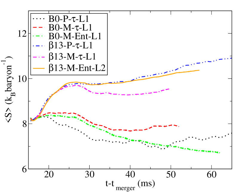
Figure 1: Comparison of the total density-averaged entropy for different numerical methods for nonmagnetized and stronger magnetized cases. The $\tau$ method for energy evolution shows extra heating happening at the late time evolution for the nonmagnetized case using both puncture and multipath methods.

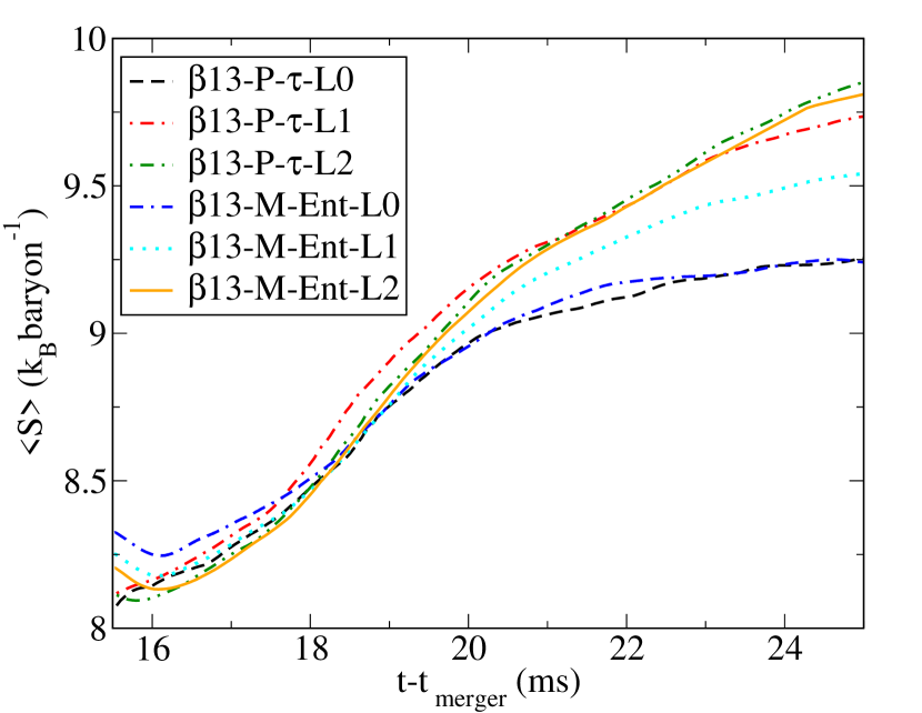
Figure 2: Convergence test on the specific entropy in the first $10\,\mathrm{ms}$ of evolution for the magnetized disk with puncture-tau and multipatch-entropy methods. A smoothing of scalar primitive variables after the interpolation onto multipatch grids causes slightly higher initial average entropy in these runs, but the difference quickly decreases and the subsequent evolutions for both methods are in good agreement at different resolutions.

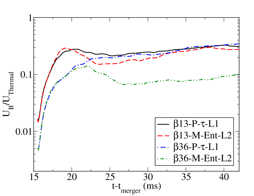
Figure 3: Comparison of the magnetic energy to the thermal energy ratio for different magnetized cases with different methods. The $\beta$36-P-$\tau$-L1 case reaches the same saturation level as the stronger field cases, but the magnetic energy starts to dissipate in the $\beta$36-M-Ent-L2 case, leading the ratio to decrease over time and finally saturate at a lower level (see table 1 for simulation labels).

We implemented two fixes to enable stable magnetized inflow into the BH. The first is to map to a new coordinate system in which the sphere $r_{\rm EX}$ is mapped to a point, so that the interior of this sphere is not on the grid (”excision by coordinates”). This method is implicitly used in non-vacuum numerical relativity moving puncture evolutions Baiotti and Rezzolla (2006); Faber et al. (2007); Liu et al. (2009) and has been explicitly used for MHD by Etienne et al Etienne et al. (2010a). We then evolve the MHD equations as in Muhlberger et al. (2014) with constrained transport and no explicit excision. We call this a “puncture” method. The second fix is to replace Cartesian grids with cubes deformed so as to fit together and fill the space between inner and outer spherical shells, the so called “cubed-sphere” configuration which has already been successfully applied by other codes to numerical relativity Thornburg (2004); Schnetter et al. (2006); Reisswig et al. (2007); Pazos et al. (2009); Pollney et al. (2011), hydrodynamics Zink et al. (2008); Korobkin et al. (2011, 2012); Reisswig et al. (2013), and MHD Koldoba et al. (2002); Fragile et al. (2009); Romanova et al. (2012). Each deformed sphere is evolved on its local coordinate system. We call this method “multipatch”. For the induction equation, we implement a centered hyperbolic divergence cleaning method. Details of these methods and code tests are provided in the Appendix.

An additional numerical challenge is posed by the nonmagnetized disk which, as it cools, becomes more supersonic. In our conservative MHD formulation, only the total energy and momentum density are evolved, so it becomes difficult to accurately extract temperature information when internal energy is much less than kinetic energy. SpEC has a procedure Muhlberger et al. (2014) for “fixing” energy and momentum evolution variables when they fail to map to any physical temperature and velocity. In previous papers, this fixing was invoked only in unimportant low density regions, but here it leads to glitches in temperature inside the high-density region of the torus and unphysical heating. We cure this problem by introducing an auxiliary entropy variable used to exclude unphysical jumps in temperature, similar to a technique used in the HARM3D code Noble et al. (2009). Details are given in the Appendix.

A list of the combinations of methods and resolutions reported in this paper is provided in Table 1. A comparison of results for the average entropy evolution is given in Fig. 1. Entropy is a particularly useful diagnostic of thermal evolution because it responds only to physical heating and cooling effects. Unlike temperature, entropy is unaffected by adiabatic expansion/compression and by nuclear reactions (if, as here, the gas remains in nuclear statistical equilibrium). We see that the methods give overall agreement, except that only simulations with the new entropy variable can maintain cooling of the nonmagnetized disk.

In Fig. 2, we test convergence of magnetized disk runs by evolving with both grid types at three resolutions. Fortunately, puncture and multipatch runs seem to converge to each other. Puncture grids have more gridpoints for a given resolution of the disk interior, but they also allow larger timesteps (because they don’t have the multipatch code’s concentration of angular grid points near the horizon).

For the nonmagnetized disk evolution, we have investigated the effect of numerical viscosity on the late-time cooling rate. We evolve in multipatch mode at three resolutions (the same as in the magnetized disk convergence test). We also perform a fourth simulation with a radial map that concentrates resolution near the maximum-density ring, increasing resolution there by a factor of 2.5. (See Appendix for details.) In all cases, the entropy curves, and especially the late-time cooling slopes, are nearly identical. We conclude that numerical viscosity cannot be an important part of the energy budget for this disk’s evolution.

In the magnetized disk simulations it is essential to resolve the MHD instabilities to capture all MHD effects. Resolving the MRI requires high resolution ($\approx 10$ grid points, to capture the growth of fastest-growing mode, along $\lambda_{\rm MRI}$ Shibata et al. (2006)). We achieve this resolution despite a modest number of grid zones by using strong seed fields and by using coordinate maps to increase the resolution in high density regions near the disk midplane as described in the Appendix. Measuring $\lambda_{\rm MRI}/\Delta x$ at the initial time shows that MRI fastest-growing mode is resolvable in over $80\%$ of the magnetized fluid (medium resolution). We find that the thermal evolution is much more sensitive to vertical than to radial resolution, presumably because it is the mode of the axisymmetric MRI with vertical wavenumber that is most significant in the high-density region, so we use grids with $\Delta z<\Delta r$.

Although it is simple to check $\lambda_{\rm MRI}/\Delta x$, it is not possible to disentangle MRI-driven field amplification from other effects. Local field amplification on the orbital time is seen–in fact, it is seen even in some regions where the MRI fastest-growing mode is certainly not resolved, as would be expected from nonmodal shearing wave amplification Squire and Bhattacharjee (2014). In our case, there is the additional complication that our initial state is not a hydrodynamic equilibrium but an extremely dynamical configuration.

Fig. 3 shows another comparison of results for the total magnetic energy to the thermal energy ratio for the magnetized cases. There is a good agreement between the puncture and multipatch methods for the stronger field case; The energy ratio grows by more than one order of magnitude and saturates at the same level for both methods. For the weaker field case, the multipatch run does not resolve MRI growth as well, so there is a larger difference. For the puncture run, the magnetic field saturates at the same level as the stronger field, indicating that the saturation state is independent of the initial seeded magnetic field (at least for our range of seed fields). The weakly magnetized-multipatch simulation (case $\beta$36-M-Ent-L2 in table 1) on the other hand, tracks the similar puncture simulation $\beta$36-P-$\tau$-L1 for about $5\,\mathrm{ms}$, and then it decreases for about $10\,\mathrm{ms}$ and finally saturates at a level that is lower by a factor of two. This shows that our puncture method can resolve the magnetic field growth better for weakly magnetized case. Based on the methods comparison and convergence studies, we present puncture simulation for the weakly magnetized case ($\beta=36$), and multipatch simulations for the nonmagnetized and strongly magnetized ($\beta=13$) cases in the next section.

IV Results

We concentrate only on the results of simulations using multipatch grid and auxiliary entropy evolution methods with moderate resolution for the nonmagnetized case (B0-M-Ent-L1), and high resolution for strongly magnetized case ($\beta$13-M-Ent-L2), and the puncture $\tau$ evolution methods for the weakly magnetized case ($\beta$36-P-$\tau$-L1) in Table 1. All grids and evolution methods give similar results for the first $\sim$25 ms, but these particular runs give more reasonable results in the subsequent evolution (see the detailed discussion in appendix A). At the initial time, the thermal timescale is estimated as $\tau_{\rm thermal}\sim E_{\rm thermal}/L_{\nu}\sim 10$ ms. We evolve for about 50 ms, long enough to see the disk altered by thermal effects.

IV.1 Dynamical evolution

In Fig. 4, we plot several global quantities of the disk. As expected, adding a magnetic field enables angular momentum transport, leading to an accretion rate roughly one order of magnitude higher than that of the disk evolved without a magnetic field. The accretion rate does not appear very sensitive to the strength of the seed field, at least for the very limited range studied here. The settled accretion rate of $\sim 0.4\,M_{\odot}\,\mathrm{s}^{-1}$ is low enough that a thermal instability is not expected Janiuk et al. (2007). MHD effects can also cause the disk to expand radially and vertically, as is expected from angular momentum transport (see the 2D images of the density profile Figs. 6 and  5 showing the nonmagnetized and magnetized disks at $t=45$ ms respectively). This transport especially drives matter into the inner radii ($r\sim 30\,\mathrm{km}$), leading to higher densities there. The nonmagnetized disk, on the other hand, contracts vertically and radially, becoming more ring-like as it loses thermal pressure support. Evolution without a magnetic field leads to a significantly denser disk, which explains why the magnetized disks have lower average temperature even though they have higher average entropy (last panel in Fig. 4).

The lower three panels of Fig. 4 show the effect of magnetic fields on the average entropy per baryon $\langle S\rangle$, electron fraction $\langle Y_{e}\rangle$, and temperature $\langle T\rangle$. Even with no magnetic field, cooling (as measured by $\langle S\rangle$) is delayed 10 ms by shock heating; once the disk has settled, it commences cooling. If a seed field is introduced, $\langle S\rangle$ increases with time. The slope for the first 10 ms is higher and quite seed field-strength dependent and should perhaps be considered a transient as the field saturates, while subsequent heating is slower and less sensitive to seed field strength.

With no magnetic field, $\langle Y_{e}\rangle$ decreases monotonically, continuing the behavior seen in our earlier simulations Foucart et al. (2014), while magnetized runs show a leveling off and slight increase. Siegel and Metzger’s 3D magnetized disk simulations also find that the inner disk remains neutron rich Siegel and Metzger (2017). Radial profiles of $Y_{e}$, displayed in Fig. 7, show that the magnetized disk has higher $Y_{e}$ mostly in a region around radius $r\approx 40$ km. This can be understood from the equilibrium electron fraction $Y_{e,eq}$. In this region, the magnetized disk has lower $\rho_{0}$ and higher $T$. As shown in Fig.18 of Foucart et al. (2014), $Y_{e,eq}$ increases with $T$ and decreases with $\rho_{0}$, so the higher $Y_{e}$ is consistent with $Y_{e,eq}$. The outer regions of the disk, on the other hand, are too cool for $Y_{e}$ to equilibrate on the simulated timescale.

Figure 8 shows gas pressure, total and poloidal magnetic pressures versus distance from the black hole at two times in the two configurations $\beta 13$ (top panel) and $\beta 36$ (bottem panlel). The toroidal field quicky grows to be the dominant component, contributing about $90\%$ of the total magnetic energy at the late time evolution for our stronger field case (as seen in either puncture or multipatch runs). This figure also shows that the total field pressure exceeds the gas pressure in the inner regions. Because of our rather large seed fields, the field can only grow one to two orders of magnitude before reaching overall equipartition with the internal energy. Strong toroidal fields can suppress the MRI, especially at low wavenumbers Pessah and Psaltis (2005), and this suppression may take place in some regions of our disk.

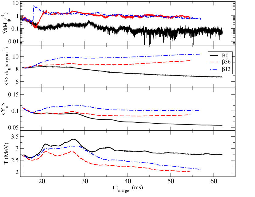
Figure 4: The evolution of the accretion rate $\dot{M}$ (first panel from the top), the electron fraction $Y_{e}$ (second panel), the specific entropy $s$ (third panel), and temperature $T$ (last panel) for magnetized $\beta$13-P-$\tau$-L1 (dashed dot line), $\beta$36-P-$\tau$-L1 (dashed line), and nonmagnetized B0-M-Ent-L1 cases (solid line). The accretion rate is higher by about one order of magnitude for the magnetized cases due to magnetorotational instablity. The entropy grows higher as a result of effective viscous heating, while the temperature decreases over time because of adiabatic cooling for the magnetized cases.

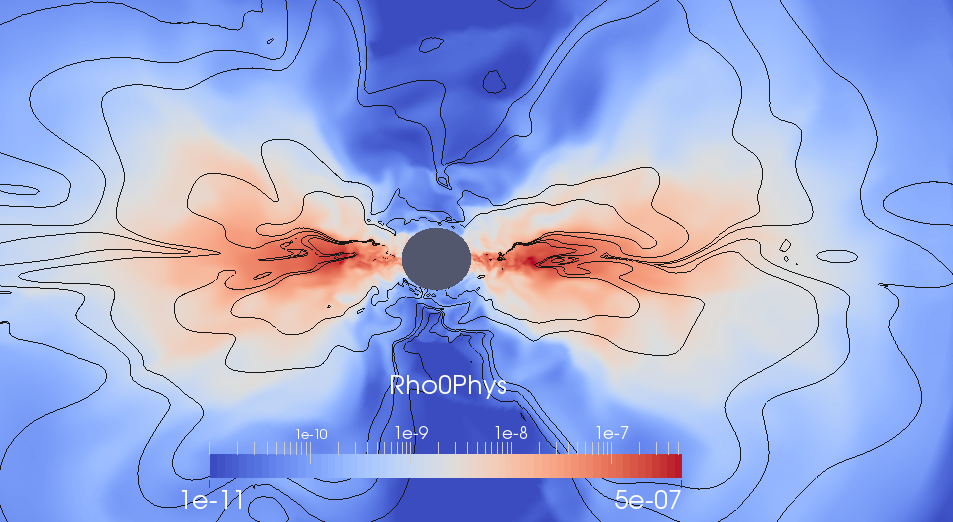
Figure 5: Snapshot of the rest-mass density in the meridional x-z plane at $t=45\,\mathrm{ms}$ for $\beta$13 case. The solid line shows magnetic field magnitude contours correspond to $\approx$ [$10^{12}$, $10^{13}$,$10^{14}$,$10^{15}$,$10^{16}$] G.

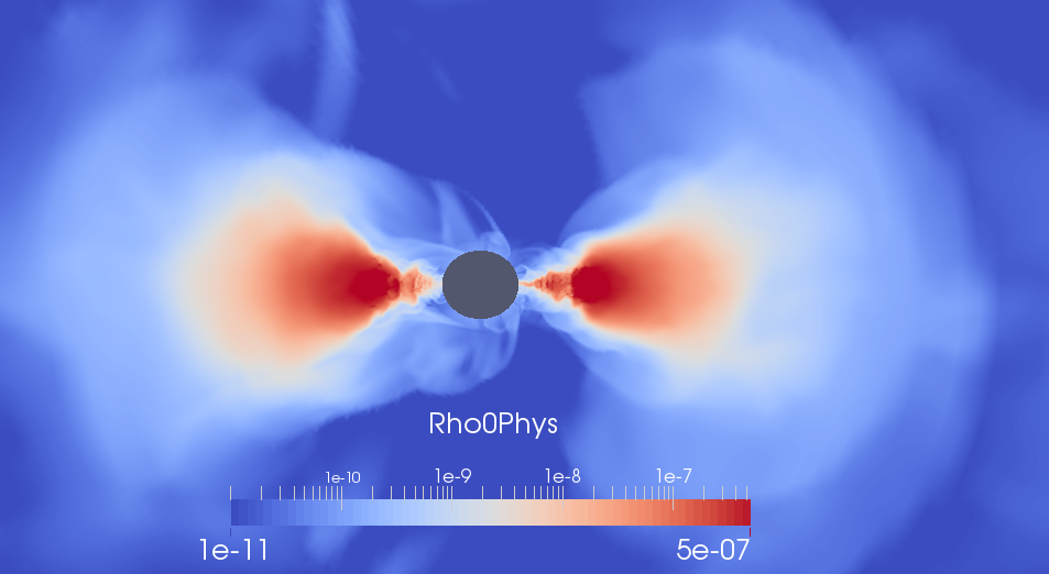
Figure 6: Snapshot of the rest-mass density in the meridional x-z plane at $t=45\,\mathrm{ms}$ for the nonmagnetized case.

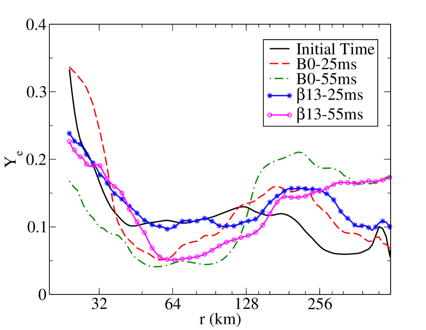
Figure 7: Vertically and azimuthally averaged electron fraction profiles at the initial time, $t=25\,\mathrm{ms}$, and $t=55\,\mathrm{ms}$. $Y_{e}$ decreases at densest regions and increases at low-density outer radii regions in nomnagnetized case. In the magnetized case, $Y_{e}$ starts decreasing in the high-density regions only at late times.

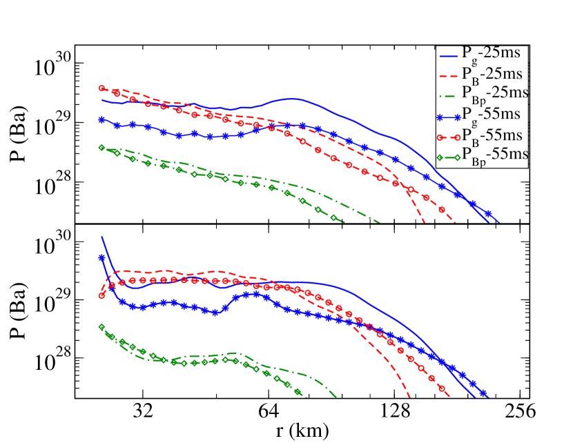
Figure 8: Vertically and azimuthally averaged radial profiles of gas pressure, total and poloidal component magnetic pressures at $t=25\,\mathrm{ms}$, and $t=55\,\mathrm{ms}$ for $\beta 13$ (top panel) and $\beta 36$ (bottom panel) magnetized cases. The toroidal component becomes dominant after the magnetic field saturates in all the magnetized cases.

IV.2 Neutrino emission and optical depth

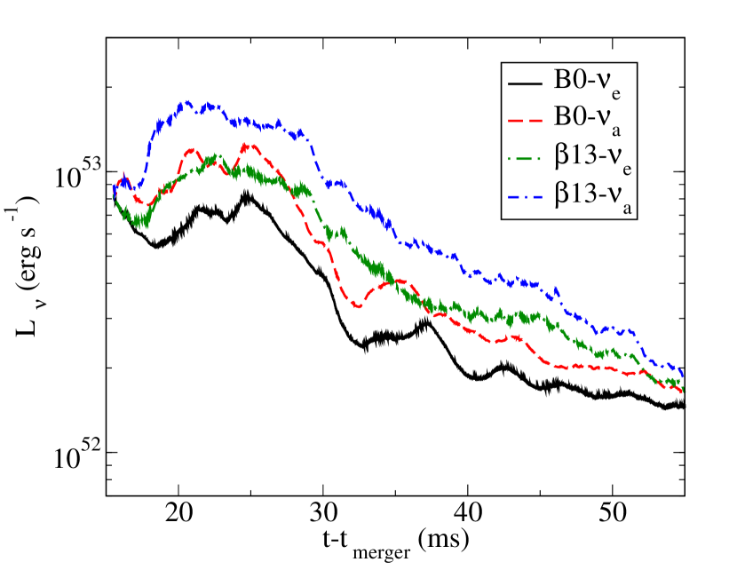
Figure 9: Neutrino luminosity evolution for electron-flavor neutrinos and antineutrinos in the $\beta=13$ and nonmagnetized simulations. The magnetized run has systematically higher electron neutrino and antineutrino luminosities.

Figure 10: The energy-averaged optical depth of electron neutrinos radial profiles at the initial time, $t=25\,\mathrm{ms}$, and $t=55\,\mathrm{ms}$. The nonmagnetized case becomes more opaque in the high-density region. This makes the neutrino cooling less efficient than in the magnetized case, which becomes more transparent during the evolution.

Fig 9 shows the neutrino luminosity for electron-flavor species. The electron antineutrino luminosity is the strongest in both the magnetized and nonmagnetized cases. The neutrino luminosity is higher in the magnetized case for all the species, but the changes are not as large as might have been expected. In all cases, the total neutrino luminosity drops from about $10^{53}\,\mathrm{erg\,s}^{-1}$ to a few times $10^{52}\,\mathrm{erg\,s}^{-1}$ over about $30\,\mathrm{ms}$ after merger. Radial emission profiles show that the luminosity drops by a comparable factor throughout the high-density region; The drop in emission does not reflect some local effect, but rather the global evolution of the disk: the contributions to the luminosity are distributed smoothly throughout the high-density region.

One possible influence on $L_{\nu}$ would be a change in the neutrino optical depth. Figure 10 plots the energy-averaged optical depth of electron neutrinos (the only neutrino flavor with optical depth sometimes greater than unity). The nonmagnetized disk maintains an optical depth of a few, while spreading of the magnetized disk makes it optically thin. Our disk has too low density to show the optically thin to optically thick transition from the inner radii to the outer radii seen in some alpha disk studies Lee et al. (2005); Janiuk et al. (2007). On the other hand, the total neutrino luminosity, and the fact that electron anti-neutrino emission is brightest, are consistent with the literature for $\alpha\sim 0.01-0.1$ disks Lee et al. (2005); Fernández and Metzger (2013).

Based on the accretion rate observations for the strongly magnetized case we estimate the equivalent $\alpha$ parameter for our disk is $\sim 0.3$. This $\alpha$ is measured from the accretion rate, which in fact, includes the angular momentum transport due to the magnetically-driven winds and the MRI turbulence. The accretion efficiency $L_{\nu}/\dot{M}c^{2}$ for the stronger magnetic field case is $\geq 15\%$. This efficiency is a few percent higher than the optically thin NDAF $\alpha$ disk models ($\alpha\approx 0.01-0.1$) with high spin black holes $a\geq 0.9$ as reported by Shibata et al. (2007) Shibata et al. (2007)

IV.3 Thermal evolution

The transport mechanism in an accretion disk affects the luminosity in two ways. By heating the disk, it tends to increase the luminosity. By spreading the disk to larger radii and lower densities and by facilitating higher accretion rates onto the black hole, it tends to decrease the luminosity. For a thin alpha disk, $\tau_{\rm thermal}\ll\tau_{\rm viscous}$, so the former effect should initially dominate, but our disk is quite thick ($H/r\approx 0.3$), so the timescales on which these effects operate are not well separated. To understand the actual disk evolution, we must quantify the major heating and cooling effects.

Figures 11, 12, and 13 show the major entropy sources and sinks for different levels of initial magnetization. From the energy and lepton number source terms provided by the leakage code, a radiative entropy sink term $\dot{S}^{-}{}_{\nu}$ can be computed (see Appendix for details). Cooling from advection into the black hole $\dot{S}^{-}{}_{Adv}$ is straightforwardly measured by monitoring entropy flux at the inner boundary. Adiabatic expansion and nuclear reactions (in nuclear statistical equilibrium) do not affect entropy, while shocks, reconnection, and turbulent dissipation should only heat. Thus, the total heating rate $\dot{S}^{+}$ should be

$$\dot{S}^{+}=\dot{S}+\dot{S}^{-}{}_{\nu}+\dot{S}^{-}{}_{Adv},$$ (2)

where $\dot{S}$ is the time derivative of the total entropy. Unfortunately, it is difficult to separate the various possible heating sources, as they will all appear in the code via the stabilizing dissipation terms in our shock-capturing MHD scheme. We normalize each source term by the instantaneous total entropy of the disk, giving the source terms the quality of inverse timescales.

The entropy budget plots Figs. 11, 12, and 13 tell a clear story. At early times, there is strong heating in all cases from shocks as the disk, still nonlinearly perturbed from equilibrium, pulsates and axisymmetrizes. This heating ceases about 30 ms after merger as the disk settles. It is especially clear in the nonmagnetized case (Fig. 11) that this happens before the neutrino luminosity drops. The neutrino luminosity drops quickly thereafter, on a fraction of the initial thermal timescale, as radiation cools the disk enough to decrease itself. This rapid cooling stops when the thermal timescale has increased to about $100$ ms.

It is worth mentioning that the unmagnetized simulations show this initial strong heating regardless of the grid and methods used. Indeed, it is seen even in the original simulation presented in Foucart et al. (2014). The exact amount of early-time heating does vary noticeably from one method to another. It is greatest for the multipatch runs, perhaps because of numerical perturbations caused by switching to a radically different grid (Fig. 1).

For the nonmagnetized case, the final state is neutrino cooling-dominated. Accretion has nearly stopped, and advective cooling is negligible. The heating rate is significantly lower than the neutrino cooling rate, although the average of the former is still around a third of the latter. Note that the heating rate does occasionally become negative, presumably a sign of numerical error in the difficult-to-follow thermal evolution of the gas as it becomes ever more supersonic. This negative heating could be removed by a stricter lower limit on the entropy (see the Appendix for details), but this would bias numerical error toward heating, which might have an undesirable cummulative effect.

For magnetized cases, the heating rate remains above the neutrino cooling rate. However, this effect is largely cancelled by the strong advective cooling that takes place as hot material accretes into the black hole. Although the component entropy sources and sinks are larger than in the nonmagnetized case, the thermal timescale in these cases also increases to $\sim$$100\,\mathrm{ms}$. At late times, the neutrino luminosity decreases slightly faster in the most highly magnetized case, although in all cases a luminosity of around $10^{52}$ erg s^-1 will be maintained till the end of the evolution.

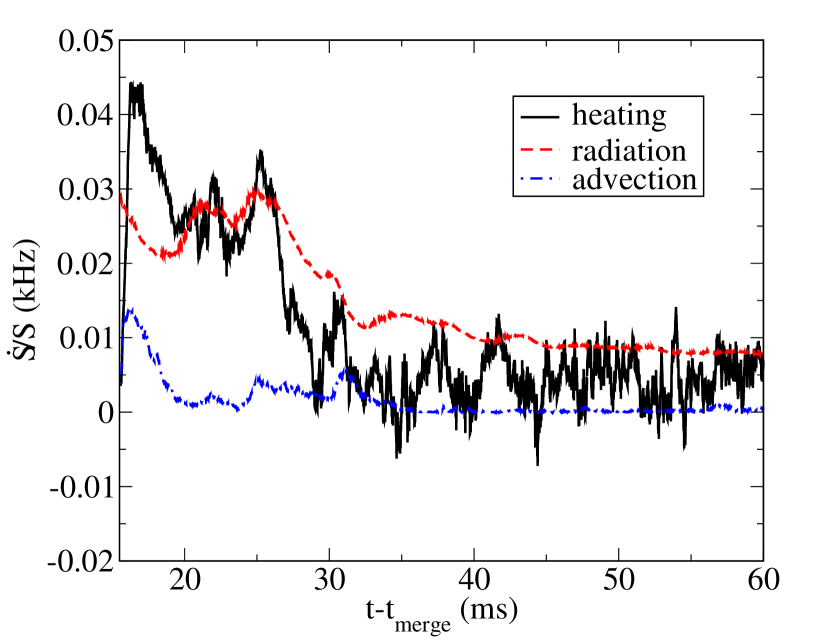
Figure 11: The evolution of the total heating rate $\dot{S}^{+}$, neutrino cooling rate $\dot{S}^{-}{}_{\nu}$ and advection cooling rate $\dot{S}^{-}{}_{Adv}$ ratios to the total entropy for the nonmagnetized case. Heating and neutrino cooling rates drop significantly around $t=30\,\mathrm{ms}$. The advection cooling is almost zero at the end of the simulation.

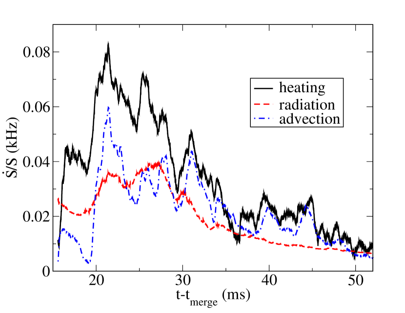
Figure 12: The evolution of the total heating rate $\dot{S}^{+}$, neutrino cooling rate $\dot{S}^{-}{}_{\nu}$ and advection cooling rate $\dot{S}^{-}{}_{Adv}$ ratios to the total entropy for the case with weaker seed field ($\beta=36$). Like in the nonmagnetized case, the total heating and neutrino cooling rates decrease significantly comparing with the early time. The advection cooling rate is considerably higher due to the MHD effects.

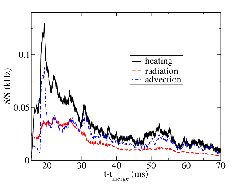
Figure 13: The evolution of the total heating rate $\dot{S}^{+}$, neutrino cooling rate $\dot{S}^{-}{}_{\nu}$ and advection cooling rate $\dot{S}^{-}{}_{Adv}$ ratios to the total entropy for the standard, stronger seed field. The disk shows the same qualitative thermal behavior as in the weaker seed field case.

In Figure 14, we plot late-time convergence for representative global quantities. Convergence at these times is difficult to achieve because it requires resolving not only the fastest-growing MRI wavelength but also sufficient inertial range that the average transport effects of turbulence are accurately captured. In the highest-resolution study to date of a BHNS post-merger system, Kiuchi et al. Kiuchi et al. (2015) were unable to demonstrate convergence even with grid spacing a few times smaller than we can afford. Thus, it is not surprising that we also obtain no better than qualitative convergence, i.e. the overall behavior is similar at all resolutions. Like Kiuchi et al., we see a tendency toward more vigorous turbulent heating at higher resolutions.

Figure 14: Convergence study of the total neutrino luminosity and heating rate for nonmagnetized and strong seed field multipatch runs. The results are qualitatively convergent in both cases.

IV.4 Comparison with previous studies

Magnetized black hole-neutron star mergers have been carried out by other groups Chawla et al. (2010); Etienne et al. (2012); Paschalidis et al. (2015); Kiuchi et al. (2015). In particular, Etienne et al. Etienne et al. (2013) have also inserted a poloidal field into a post-merger BHNS disk. The highest-resolution MHD BHNS merger simulation is that of Kiuchi et al Kiuchi et al. (2015). These simulations, like ours, have more realistic initial disk profiles than analytic tori would provide. However, there are important differences in our treatment of the thermal evolution of the disk. The above-mentioned studies, since they did not employ a finite-temperature nuclear equation of state, did not include neutrino cooling, which is present in our simulations, so their disks were presumably too hot. On the other hand, by inserting a seed field only when it was safe to apply the Cowling approximation, our disk had cooling for 15 ms without one of the major heating sources, so our disk is likely over-cooled. Furthermore, the convergence studies in Kiuchi et al. (2015) find that heating in the inner disk is very resolution dependent, with insufficient resolution leading to underestimates of thermally driven outflows in particular. A truly realistic thermal state of the disk would presumably be somewhere in between these extremes. (Of course, a truly realistic treatment would also require neutrino transport, not just a leakage approximation.)

Both the Etienne et al poloidal seed study and the highest-resolution simulations of Kiuchi et al Kiuchi et al. (2015) find sustained Blandford-Znajek Poynting flux polar jets. Our MHD disk evolutions do produce some unbound outflow over the simulation period ($M_{\rm ub}\sim 10^{-5}M_{\odot}$, average $\dot{M}_{\rm ub}\sim 10^{-3}M_{\odot}$ s^-1) and a magnetically-dominated polar region, but the polar field does not organize itself into a radial Blandford-Znajek like structure. The above-mentioned differences in thermal treatment in our simulation and resolution effects may play a role here. However, we also find that the presence or absence of strong winds and Poynting flux outflows is sensitive to the choice of seed field. When we evolve with a less confined initial field, we do see stronger matter outflow and polar magnetic flux. One might worry that these effects could somehow be suppressed by too strong a seed field, but simulations of neutrino-cooled disks with analytic initial conditions all find that stronger fields (as high as $\langle\beta\rangle\sim 5$) yield stronger winds and stronger Blandford-Znajek luminosity Janiuk et al. (2013). Even these analytic disks with weaker initial magnetic field ($\langle\beta\rangle\sim 200$) find strong unbounded outflows after evolving the magnetized disk long enough Siegel and Metzger (2017), and this might also turn out to be the case for our more confined B-field evolutions if evolved longer.

V Conclusions

We have carried out simulations of a BHNS post-merger system with a realistic initial state provided by a numerical relativity merger simulation , including both neutrino emission effects and magnetic field evolution. The initial magnetic field is applied as large poloidal loops confined in the post-merger disk. Because our simulations include the major heating and cooling sources, we can study the contribution of each thermal driving process as the disk settles toward thermal equilibirum. Without a magnetic field, there is no such thermal equilibrium, so after an initial phase of shock heating, the disk enters a phase of long-term cooling by neutrinos. With a strong seed magnetic field, the final state after several initial thermal timescales is a rough balance between MHD-related heating and advective cooling, with neutrino cooling being a secondary effect, driving the entropy down over longer timescales. This is roughly consistent with the long term evolution of two dimensional neutrino cooled $\alpha$-viscosity disks reported by Fernandez et al. Fernández et al. (2015), where neutrino cooling is only important at early times. In both magnetized and nonmagnetized cases, the main reason for settling is not a precise achievement of equilibrium, but an increase in the thermal timescale (from $\sim 10$ ms to $\sim 100$ ms) as the initially-high neutrino luminosity drops.

The considered magnetized 3D BHNS post-merger configuration provided the opportunity to test multiple methods for evolving the relativistic MHD equations. These show reassuring consistency over the first $\approx 20$ ms, but realistic long-term evolution requires careful treatment of the energy variable, especially in how one handles the problematic recovery of primitive variables. The multipatch methods employed in some of our simulations can easily be applied to more general grid configurations Pazos et al. (2009).

The initial study of magnetized 3D BHNS post-merger disk evolution presented in this paper is limited in many ways. Only one BHNS system and one magnetic seed field geometry were used. Neutrino effects might be different for an opaque disk (e.g., Deaton et al. (2013)), and magnetohydrodynamic effects are known to be seed field-dependent Beckwith et al. (2008). Our leakage scheme neglects neutrino absorption, which could smooth temperature profiles and launch winds. Existing neutrino transport codes (e.g., Foucart et al. (2015)) can in the future be used to capture these effects. Finally, it would be interesting to carry out a similar study on NSNS post-merger systems.

Appendix A Numerical improvements

A.1 Formulation

The fundamental equations to be evolved are the same as in our earlier MHD work Muhlberger et al. (2014). We write the metric

$$ds^{2}=-\alpha^{2}dt^{2}+\gamma_{ij}(dx^{i}+\beta^{i}dt)(dx^{j}+\beta^{j}dt).$$ (3)

The fluid at each grid point is described by its set of “primitive variables”: baryonic density $\rho_{0}$, temperature $T$, electron fraction $Y_{e}$, and spatial components of the covariant 4-velocity $u_{i}$. From $\rho_{0}$, $T$, and $Y_{e}$, the equation of state supplies the gas pressure $P$, specific enthalpy $h$, and sound speed $c_{s}$. From $u\cdot u=-1$, we know the Lorentz factor $W=\alpha u^{t}$. The stress tensor is

$$T_{ab}=\rho_{0}hu_{a}u_{b}+Pg_{ab}+F_{ac}{F_{b}}^{c}-\frac{1}{4}F^{cd}F_{cd}g_{ab}\ ,$$ (4)

where $F_{ab}$ is the Faraday tensor. We assume a perfectly conducting fluid, $F^{ab}u_{b}=0$, which fixes the electric field. The variables actually evolved (aside from the magnetic field, whose evolution is described below) are the conservative variables: a density variable $\rho=\sqrt{\gamma}W\rho_{0}$, the proton density $\rho Y_{e}$, an energy density variable $\tau=\sqrt{\gamma}\alpha^{2}T^{00}-\rho$, and a momentum density variable $S_{i}=\sqrt{\gamma}\alpha T^{0}{}_{i}$. In the above, $\gamma$ is the determinant of the spatial metric. We evolve using an HLLE approximate Riemann solver Harten et al. (1983). Conservative formulations have the advantage that numerical dissipation in shock or turbulent subscale structures is automatically conservative. They have the disadvantage of not evolving a separate variable for the internal energy or entropy. Such information must be recovered by root finding from the conservative variables after each timestep, which can be expensive and (especially if kinetic energy dominates over internal energy in $\tau$) inaccurate.

The magnetic field can be described via the components of its 2-form $\tilde{B}^{i}$ or its vector field $B^{i}$, related as $\tilde{B}^{i}=\sqrt{\gamma}B^{i}$. In a conducting medium, field lines advect with the fluid: $\partial_{t}\tilde{\bf B}=-\pounds_{v}\tilde{\bf B}=-d(v\cdot\tilde{\bf B})$. Since $d\tilde{B}=0$, we can alternatively evolve the vector potential 1-form ${\bf A}$, where $\tilde{\bf B}=d{\bf A}$. A vector potential evolution will automatically satisfy $d\tilde{B}=0$ but will require specifying a gauge.

Our Cartesian grid simulations suppress monopoles via a constrained transport scheme, which requires staggering $\tilde{B}^{i}$ or $A_{i}$ between gridpoints. For the multipatch simulations described below, this would be very inconvenient because the patch coordinate transformations would have to account for each component of the field being at a different location, so we instead code two well-known methods that control $d\tilde{B}$ while keeping all variables centered at the same gridpoints. The first is a centered vector potential method, implemented as in Giacomazzo et al. (2011). We find that the generalized Lorentz gauge, introduced in Farris et al. (2012), provides the best stability. The evolution for $A_{i}$ and the scalar potential $\Phi$ are given by

$$\partial_{t}A_{i} = \epsilon_{ijk}v^{j}B^{k}-(\alpha\Phi-\beta^{j}A_{j})_{,i},$$ (5)

$$\partial_{t}(\sqrt{\gamma}\Phi) = -\partial_{j}(\alpha\sqrt{\gamma}A^{j}-\sqrt{\gamma}\beta^{j}\Phi)-\xi\alpha\sqrt{\gamma}\Phi\ ,$$ (6)

where $\xi$ is a specifiable constant of order the mass of the system. Lorentz-type gauges lead to luminal characteristic speeds, but fortunately the speeds used in the HLLE fluxes used in the evolution of $A_{i}$ (see Giacomazzo et al. (2011)) can still be set to the physical, MHD wave maximum speed. The signal speeds for HLLE fluxes in the $\Phi$ evolution, on the other hand, are set to the null $-\beta^{i}\pm\alpha\gamma^{ii}$.

The second magnetic evolution scheme is a covariant hyperbolic divergence cleaning method Liebling et al. (2010); Penner (2011); Mösta et al. (2014), in which an auxiliary evolution variable $\Psi$ is introduced to damp monopoles. The Maxwell equation $d{\bf F}=0$ is replaced by $\star d{\bf F}={\bf g}\cdot d\Psi-\lambda\Psi{\bf t}$, where ${\bf g}$ is the 4-metric, ${\bf F}$ the Faraday tensor, ${\bf t}$ the unit time vector, and $\lambda$ a specifiable damping constant. In components

$$\partial_{t}\tilde{B}^{i} = \partial_{i}(v^{j}\tilde{B}^{i}-v^{i}\tilde{B}^{j})+\alpha\sqrt{\gamma}\gamma^{ij}\Psi_{,j}+\tilde{B}^{j}{}_{,j}\beta^{i},$$ (7)

$$\partial_{t}\Psi = \beta^{i}\Psi_{,i}-\alpha\gamma^{-1/2}\tilde{B}^{j}{}_{,j}-\lambda\Psi,$$ (8)

where we set $\lambda=1.4$. Eq. 7 is in conservative form and can be evolved using our usual HLLE scheme, while Eq. 8 is evolved via straightforward second-order centered finite differencing.

Both of these methods require added numerical dissipation. Thus, we add Kreiss-Oliger dissipation to the magnetic evolution equations. For multipatch simulations, this step is done while time derivatives are being computed in the local patch coordinate system of evolution variable components in these coordinates.

$$\partial_{t}X=\cdots-\Sigma_{i}\Delta x_{i}^{3}D_{2i}(FD_{2i}X)\ .$$ (9)

$X$ is $(\tilde{B}^{i},\Psi)$ for divergence cleaning and $(A_{i},\Phi)$ for the vector potential method. $D_{2i}$ is a second-derivative operator, and $\Delta x_{i}$ is the grid spacing in the $i$-th direction, both computed in local patch coordinates. $F$ is a function of space, which vanishes on boundary points but may be otherwise chosen according to the problem Mattsson et al. (2004).

A.2 Cubed-sphere Multipatch Grids

Several groups have already implemented dynamics on spherical surfaces Sadourny (1972); Ronchi et al. (1996), 3D hydrodynamics Zink et al. (2008); Korobkin et al. (2011, 2012); Reisswig et al. (2013), 3D MHD Koldoba et al. (2002); Fragile et al. (2009); Romanova et al. (2012), and Einstein’s equations Thornburg (2004); Schnetter et al. (2006); Reisswig et al. (2007); Pazos et al. (2009); Pollney et al. (2011) with multipatch methods and cubed-sphere-like grids. The basic idea is to divide the computational domain into patches, each of which has its own local coordinate system in which it is a uniform Cartesian mesh. In the global coordinate system, each patch is distorted, and six distorted cubes can be fit together to fill a volume with spherical inner and outer boundaries. Time derivative calculations for timesteps are computed within the local patch coordinates and then transformed to the global coordinate system. Multipatch methods easily generalize to any combination of distorted cubes. For example, the central hole can be filled with a cube (as done in a test problem below), or the cubed-sphere could be surrounded by non-distorted cubes.

This method can be contrasted with other popular ways of evolving grids around black holes. One is the use of spherical-polar coordinate grids. The second is the use of Cartesian grids, with removal of the black hole interior accomplished either by excising all gridpoints within a spherical region (leading to an irregular-shaped “legosphere”) or by removing the interior via a radial coordinate transformation (“puncture”) Etienne et al. (2010b). All previous SpEC black hole-neutron star simulations use Cartesian grids with legosphere excision. We have been unable to find a stable implementation of this method for magnetized flows into a black hole. This is not surprising, since Cartesian grid faces even inside the horizon will have characteristic fields flowing into the grid, making the evolution ill-posed without boundary conditions providing information about the excised interior. Both spherical-polar and multipatch grids can naturally excise spherical regions (which can be distorted by coordinate transformations to fit the horizon shape as needed) and have no incoming characteristics if placed inside the apparent horizon (and outside the Cauchy horizon) of a stationary black hole. Multipatch methods have an advantage over spherical-polar grids that they do not suffer from coordinate singularities and grid pileup near the poles, which can be an issue for high-resolution spherical-polar simulations Shiokawa et al. (2012). Spherical-polar grids, on the other hand, have two advantages. First, for nearly axisymmetric systems, one can have much lower resolution in longitude than in latitude, a freedom not present in multipatch grids. Second, communication between patches in multipatch grids is by ghost zone overlaps. Ghost zone gridpoints will not match gridpoints on the overlapping live patch, so they must be filled by interpolation. This introduces a new source of error which will generally not exactly respect conservation laws and may create magnetic monopoles, although it should converge away with resolution. Which method is best most likely depends on the problem.

Since our conservative evolution equations are generally covariant, it is straightforward to evolve them in the local patch coordinates, shifting to global coordinates for ghost zone synchronization. For our WENO5 reconstruction method, we need three ghost zone layers on patch interior boundaries. Because of our methods of “fixing” problematic points described below, synchronizing variables is not quite the same as just synchronizing their time derivatives, and we find the former to be needed for stability. For the divergence cleaning method, any monopoles generated by interpolation of $\tilde{B}^{i}$ in ghost zones are damped (by design of Eqs 7 and 8) and remain small. For the vector potential method, we synchronize $\tilde{B}^{i}$ computed from $A_{i}$ on patch faces, where information is lacking on one side to compute the curl. It is crucial here to synchronize only the outermost layer of points, not the full 3-layer ghost zone region, because the latter will introduce monopoles in the ghost zones and lead rapidly to an instability there.

Our cubed-sphere grids are largely the same as those of other groups. A minor alteration in the ghost zones is illustrated in Fig. 15 to eliminate the presence of overlap regions which are “live” for both grids (i.e. neither is synced with respect to the other). Our fears that “live overlaps” would be dangerous have not been borne out, but the new arrangement does seem to propagate shocks a bit better and show less deviation in rest mass (interpolated ghost zones do not allow strict mass conservation in either case), although it cannot be generalized to more general multipatch structures.

Figure 15: An illustration of the synchronization of ghost zone regions at internal patch boundaries. As is standard practice with uniform grids, one grid is extended the full ghost zone width (three points, in our case) beyond the interface, while the other grid extends two points. For a cubed spheres setup, ghost zone extensions must be chosen to guarantee sufficient overlaps on 3-patch edges. Above, open circles are ghost zone points; filled circles are live points. The points B and H overlap and mark the interface. First H is set to B (which does not require interpolation). Then H can be used in the interpolation to get C.

Figures 16, 17, and 18 show some standard MHD test problems applied to the multipatch MHD code. Fig. 16 is the first Riemann problem from Balsara (2001) and Giacomazzo and Rezzolla (2007), containing a left-going fast rarefaction wave, a left-going compound wave, a contact discontinuity, a right-going slow shock and a right-going fast rarefaction wave. To test relativistic terms, we set lapse $\alpha=0.5$ and shift $\beta^{n}=0.1$, yielding the expected slowdown and advection. A cubical patch is added to the center to fill the inner hole, while the planar symmetry is imposed on the outer boundary, setting functions in the outer points to their values at the closest point in the interior on a line in the symmetry plane. The waves travel through interpolated boundaries without incident.

In Fig. 17, we evolve a Bondi accretion problem (the same as in Muhlberger et al. (2014)) with a radial magnetic field and maximum $\beta^{-1}$ of 2.5. Both of these tests are performed with the divergence cleaning code. As in our earlier paper Muhlberger et al. (2014), we find better behavior when we add Kreiss-Oliger dissipation to all variables, with $F=0.06r^{-2}$. Errors saturate after a few $M$ of evolution, with second-order convergence demonstrated except at the sonic point and the inner boundary.

Finally, we evolve a constant angular momentum Fishbone-Moncrief torus  Fishbone and Moncrief (1976) around a rapidly spinning black hole. We set the dimensionless spin of the black hole to $a/M_{\rm BH}=0.938$, the angular momentum parameter to $\ell=4.281$ ($\ell=u^{t}u_{\phi}$), average $\beta=100$, and the equation of state to a Gamma law with $\Gamma=4/3$, making the problem very similar to a standard scenario studied by the HARM code McKinney and Gammie (2004); Shiokawa et al. (2012). We use the same radial and angular coordinate maps as in these studies. Like in Fragile et al. (2009), we find that it is necessary to tilt the grid in order for the current sheet formed by winding of the seed field to break in a reasonable time and initiate turbulence. We agree with their observation that this is an artifact of symmetries in the setup and should not be a worry for general problems. Fig. 18 shows on the left a snapshot of the density at $t=1600M$, on the right a representation of the grid with resolution quartered for clarity. The actual evolution grid used 120 radial points and 60 angular points across each of the six patches. For this problem, we found it advantageous to have higher dissipation in problematic regions (low density regions and the viscinity of the black hole) and low dissipation inside the torus, where we wanted to resolve the MRI with modest resolution. There we set $F=0.01$ ($F=0.001$) inside the disk for $X=\tilde{B}^{i}$ ($X=A_{i}$), and we set $F=0.1$ for $\rho_{0}/\rho_{0\rm max}<0.05$ or $r/M_{\rm BH}<3$. Results qualitatively match the literature, with mass flow into the horizon $<\dot{M}>\sim 1$, electromagnetic energy flux out of the horizon $<L_{\rm EM}>\sim 10^{-2}\dot{M}$, and the generation of unbound matter.

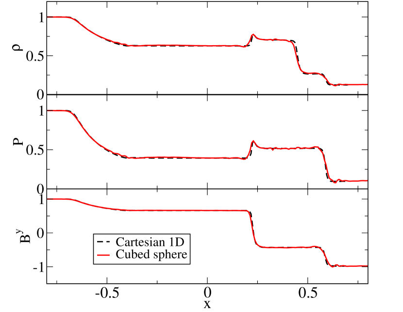
Figure 16: Magnetized Riemann problem evolved on both a cubed-sphere multipatch grid (with about 240 grid points across the diameter of the spherical computational domain), together with the results for the same problem evolved on a Cartesian one-dimensional grid which is able to utilize the planar symmetry. The interface between the inner cube and outer cubed spheres is at $\pm$ 0.27.

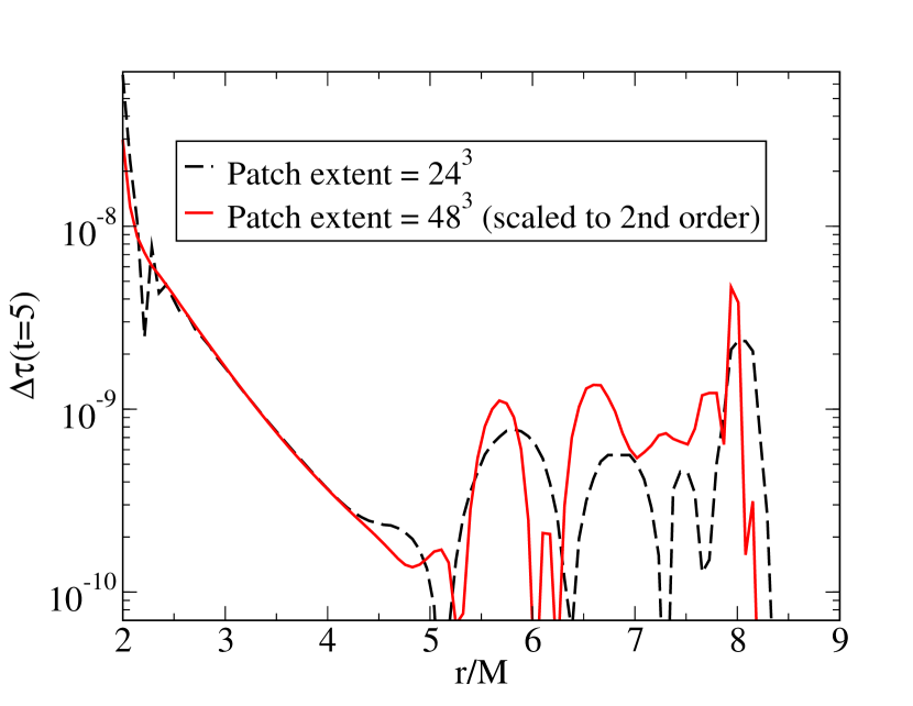
Figure 17: Convergence test for Bondi accretion with a radial magnetic field. Shown here is the error in the $\tau$ conservative variable at $t=5M$, by which time it has settled. The error plotted is the absolute change in $\tau$. The relative change of $\tau$ is about $2\times 10^{-4}$ at the lower resolution. Second-order convergence breaks down at the sonic radius at $r=8$, as expected. The grid consists of 48 domains, with each of the six patches split in two on each of its axes.

Figure 18: Meridional snapshot at $t=1600M$ of a turbulent accretion torus. Shown on the left is the density (on a logarithmic scale covering the four decades up to the maximum). On the right is the grid, with resolution reduced by about a factor of 4 for clarity. The effects of the radial and angular maps are visible, as is the regularity of the poles. The unusually close radial lines are nonmatching ghost zones.

A.3 Coordinate maps

In its fluid module, SpEC assumes uniform grid spacing in the coordinates on which the grid is defined, so nonuniformity can be acheived by introducing coordinate transformations between these grid coordinates and the original, “physical” coordinates. All simulations use logarithmic radial maps [i.e. uniform spacing in $\log(r)$], concentrating grid near the black hole. For Cartesian simulations, this naturally introduces a puncture, set at the desired excision radius $r_{\rm EX}$. It leads to enormous distortions on the edges of the cubical grid, but since we only evolve in a sphere contained by the cube, this causes no problems. For multipatch simulations, the exponential map preserves the ratio between radial and transverse grid spacings; both increase with distance from the center.

We also add maps to concentrate grid near the equator. For multipatch runs, we use the angular map common for MHD disk simulations $\theta=\pi\theta^{\prime}+(1-h)\sin(2\pi\theta^{\prime})/2$  McKinney and Gammie (2004) with $h=0.4$. For Cartesian runs, this angular map unacceptably distorts grid cells, leading to artifacts in the evolution, so we instead use a cubic scale map on the z axis ($Z=z-\lambda(z-R_{min})^{3}/R_{min}^{2}$ with $\lambda=-0.375$ and $R_{min}=1.0$).

Finally, we have carried out multipatch simulations using a radial map (composed with the logarithmic map) to concentrate grid on a ring coinciding with the high-density region. The map has the form

$$r^{\prime}-r_{0}=A\arctan\left[\frac{r-r_{0}}{\lambda}\right]+B(r-r_{0})+C(r-r_{0})^{2}\ ,$$ (10)

where $r$ is the grid radius, $r^{\prime}$ the physical radius, $\lambda$ controls the width of the zoomed region, while $A$, $B$, and $C$ are set so that $r$ and $r^{\prime}$ coincide at the inner and outer radii, and the appropriate zoom factor ($dr^{\prime}/dr$) is acheived at $r^{\prime}=r=r_{0}$.

A.4 Primitive variable recovery

Sometimes, due to numerical error, the evolved conservative variables $(\rho,\rho Y_{e},\tau,S_{i},\tilde{B}^{i})$ may not correspond to any physical $(\rho_{0},T,Y_{e},u_{i},B^{i})$. In this case, we can “fix” the conservative variables to make primitive variable recovery possible using the prescription described in Appendix A of Muhlberger et al. (2014) (straightforwardly altered to take into account the minimum of $h$ being less than one Deaton et al. (2013)). Unfortunately, this introduces glitches in supersonic flows such as those in thin disks, usually seen as gridpoints at which the temperature discontinuously jumps to the equation of state table minimum. Although this is initially a cooling effect, the glitches create artificial heating. For nonmagnetized disk simulations, this ultimately stalls the cooling of the disk after only a small decrease in total entropy.

We remove this problem by introducing an auxiliary entropy evolution variable $\rho S$, where $S$ is the entropy per baryon. The use of entropy variables to reset problematic gridpoints and ameliorate accuracy problems in the evolution of internal energy by conservative codes has already been tried by other groups Balsara and Spicer (1999); Ruffert et al. (2001); Koldoba et al. (2016).

In the absence of subgrid-scale energy dissipation (shocks, reconnection, turbulence), the entropy of a fluid in nuclear statistical equilibrium evolves by advection and neutrino emission only Shapiro and Teukolsky (1983); Ruffert et al. (2001).

$$\partial_{t}(\rho S)+\partial_{i}(\rho Sv^{i})=\frac{m_{n}\alpha\sqrt{\gamma}}{k_{B}T}[Q_{\nu}-R_{\nu}(\mu_{e}+\mu_{p}-\mu_{n})]$$ (11)

where $Q_{\nu}$ and $R_{\nu}$ are the net neutrino energy and lepton number emission rates per volume, respectively, $m_{n}$ is the nucleon mass, and $\mu_{X}$ are chemical potentials. Note that, since we have excluded only heating effects, the evolved $\rho S$ gives a lower bound on the true entropy.

Roughly speaking, we now have two energy variables, $\tau$ and $\rho S$, which are made to be consistent with each other at the beginning of each timesetep. Each step, we execute the following procedure.

1. Evolve $(\rho,\rho Ye,\rho S,\tau,S_{i},\tilde{B}^{i})$ using an HLL approximate Riemann solver. $\rho S$ must be evolved with a monotonic reconstructor to avoid new extrema. We use a second-order monotonized centered (MC2) limiter van Leer (1977). The other variables can be evolved with higher-order reconstruction like WENO.

2. Compute $S$, $Y_{e}$, and $B^{i}$ from the appropriate divisions of the conservative variables.

3. If not, attempt to solve $(T,W^{2})$ using $\tau$ and the other conservative variables except $\rho S$ using the gnewton method as implemented by the GSL Scientific Library et al .

4. If a root is found, use it to compute the entropy, $S_{\tau}$. If $S_{\tau}>\chi S$, accept the root. The parameter $\chi\leq 1$ but is otherwise freely specifiable. We use $\chi=0.97$.

5. If a root was not found, or if it violates the condition in step 4, first check to see if the point is in the force-free regime. If so, use force-free recovery of $(T,W)$. (See Muhlberger et al. (2014) for details on this solver and the conditions for its use.)

6. If the point does not meet the force-free conditions, attempt to solve for $(T^{3},W^{2})$ using $\rho S$ and the other conservative variables except $\tau$, again using GSL’s gnewton. If a root was found in step 4, use it as the initial guess for the root solve. (Using $T^{3}$ instead of $T$ speeds up convergence in some difficult points, but probably makes little difference in general.)

7. If a root could not be found with multidimensional root finding, attempt again with $\rho S$ and other variables except $\tau$, this time with GSL’s 1D brent root finder. Here we regard $W$ as the variable, solving Eq. (A24) of Muhlberger et al. (2014), with $T$ solved via a separate 1D solve of the condition $S=S(\rho_{0},T,Y_{e})$ on each iteration. This 1+1D solving is much slower but more robust than the 2D solver.

8. If this fails, attempt a 1D bracketing algorithm for $h\rho_{0}W^{2}$ which uses $\tau$ rather than $S$. (See Appendix A of Muhlberger et al. (2014)). If this fails, terminate the evolution with an error.

9. If an acceptable root was found, apply other “atmosphere” fixes to the primitive variables at low densities: limits to the temperature and Lorentz factor in these regions.

10. Recompute all conservative variables from these final primitive variables. $\tau$ and $\rho S$ are now again consistent.

A simple sanity check on our implementation of the source terms in Eq. 11 is to alter the above to force the code to always use the evolved $S$ in primitive variable recovery, in which case one observes the disk cooling on a timescale of the total thermal energy divided by neutrino luminosity.

In Fig. 1, we have already shown the difference this method makes to the entropy evolution of the nonmagnetized disk. Significantly, all discontinuous artifacts are gone when the new method is used. Because the magnetized disk does not reach such low entropies, the choice of methods makes little difference for those simulations.

References

- Nakar (2007) E. Nakar, Phys. Rep. 442, 166 (2007), arXiv:astro-ph/0701748 .
- Berger (2014) E. Berger, Ann. Rev. Astron. Astrophys. 52, 43 (2014), arXiv:1311.2603 [astro-ph.HE] .
- Popham et al. (1999) R. Popham, S. E. Woosley, and C. Fryer, Astrophys. J. 518, 356 (1999), arXiv:astro-ph/9807028 [astro-ph] .
- Di Matteo et al. (2002) T. Di Matteo, R. Perna, and R. Narayan, Astrophys. J. 579, 706 (2002), arXiv:astro-ph/0207319 .
- Janiuk et al. (2004) A. Janiuk, R. Perna, T. Di Matteo, and B. Czerny, Mon. Not. Roy. Astron. Soc. 355, 950 (2004), arXiv:astro-ph/0406362 .
- Paczynski (1991) B. Paczynski, Acta Astronomica 41, 257 (1991).
- Jaroszynski (1996) M. Jaroszynski, Astron. Astrophys. 305, 839 (1996), arXiv:astro-ph/9506062 [astro-ph] .
- Richers et al. (2015) S. Richers, D. Kasen, E. O’Connor, R. Fernandez, and C. D. Ott, Astrophys. J. 813, 38 (2015), arXiv:1507.03606 [astro-ph.HE] .
- Just et al. (2016) O. Just, M. Obergaulinger, H. T. Janka, A. Bauswein, and N. Schwarz, Astrophys. J. 816, L30 (2016), arXiv:1510.04288 [astro-ph.HE] .
- Blandford and Znajek (1977) R. D. Blandford and R. L. Znajek, Mon. Not. Roy. Astr. Soc. 179, 433 (1977).
- Meszaros and Rees (1997) P. Meszaros and M. Rees, Astrophys.J. 482, L29 (1997), arXiv:astro-ph/9609065 [astro-ph] .
- Shakura and Sunyaev (1973) N. I. Shakura and R. A. Sunyaev, in X- and Gamma-Ray Astronomy, IAU Symposium, Vol. 55, edited by H. Bradt and R. Giacconi (1973) p. 155.
- Lee et al. (2005) W. H. Lee, E. Ramirez-Ruiz, and D. Page, Astrophys. J. 632, 421 (2005), arXiv:astro-ph/0506121 .
- Dessart et al. (2009) L. Dessart, C. D. Ott, A. Burrows, S. Rosswog, and E. Livne, Astrophys. J. 690, 1681 (2009), arXiv:0806.4380 .
- Perego et al. (2014) A. Perego, S. Rosswog, R. M. Cabezón, O. Korobkin, R. Käppeli, A. Arcones, and M. Liebendörfer, Mon. Not. Roy. Astr. Soc. 443, 3134 (2014), arXiv:1405.6730 [astro-ph.HE] .
- Masada and Sano (2008) Y. Masada and T. Sano, Astrophys. J. 689, 1234 (2008), arXiv:0808.2338 .
- Guilet et al. (2015) J. Guilet, E. Mueller, and H.-T. Janka, Mon. Not. Roy. Astron. Soc. 447, 3992 (2015), arXiv:1410.1874 [astro-ph.HE] .
- Foucart et al. (2015) F. Foucart, E. O’Connor, L. Roberts, M. D. Duez, R. Haas, L. E. Kidder, C. D. Ott, H. P. Pfeiffer, M. A. Scheel, and B. Szilagyi, Phys. Rev. D91, 124021 (2015), arXiv:1502.04146 [astro-ph.HE] .
- Kiuchi et al. (2015) K. Kiuchi, Y. Sekiguchi, K. Kyutoku, M. Shibata, K. Taniguchi, and T. Wada, Phys. Rev. D 92, 064034 (2015), arXiv:1506.06811 [astro-ph.HE] .
- Deaton et al. (2013) M. B. Deaton, M. D. Duez, F. Foucart, E. O’Connor, C. D. Ott, L. E. Kidder, C. D. Muhlberger, M. A. Scheel, and B. Szilágyi, Astrophys. J. 776, 47 (2013), arXiv:1304.3384 [astro-ph.HE] .
- Foucart et al. (2014) F. Foucart, M. B. Deaton, M. D. Duez, E. O’Connor, C. D. Ott, R. Haas, L. E. Kidder, H. P. Pfeiffer, M. A. Scheel, and B. Szilágyi, Phys. Rev. D 90, 024026 (2014), arXiv:1405.1121 [astro-ph.HE] .
- Ruffert et al. (1996) M. Ruffert, H.-T. Janka, and G. Schaefer, Astron. Astrophys. 311, 532 (1996), astro-ph/9509006 .
- Rosswog and Liebendörfer (2003) S. Rosswog and M. Liebendörfer, Mon. Not. Roy. Astr. Soc. 342, 673 (2003), arXiv:astro-ph/0302301 [astro-ph] .
- O’Connor and Ott (2010) E. O’Connor and C. D. Ott, Class. Quantum Grav. 27, 114103 (2010), arXiv:0912.2393 [astro-ph.HE] .
- Shibata et al. (2011) M. Shibata, K. Kiuchi, Y. Sekiguchi, and Y. Suwa, Progress of Theoretical Physics 125, 1255 (2011), arXiv:1104.3937 [astro-ph.HE] .
- Balbus and Hawley (1998) S. A. Balbus and J. F. Hawley, Reviews of Modern Physics 70, 1 (1998).
- Hawley et al. (1995) J. F. Hawley, C. F. Gammie, and S. A. Balbus, Astrophys. J. 440, 742 (1995).
- De Villiers and Hawley (2003) J.-P. De Villiers and J. F. Hawley, Astrophys.J. 592, 1060 (2003), arXiv:astro-ph/0303241 [astro-ph] .
- McKinney and Gammie (2004) J. C. McKinney and C. F. Gammie, Astrophys. J. 611, 977 (2004), arXiv:astro-ph/0404512 .
- Chawla et al. (2010) S. Chawla, M. Anderson, M. Besselman, L. Lehner, S. L. Liebling, et al., Phys. Rev. Lett. 105, 111101 (2010), arXiv:1006.2839 [gr-qc] .
- Etienne et al. (2012) Z. B. Etienne, Y. T. Liu, V. Paschalidis, and S. L. Shapiro, Phys. Rev. D 85, 064029 (2012), arXiv:1112.0568 [astro-ph.HE] .
- Etienne et al. (2013) Z. B. Etienne, Y. T. Liu, V. Paschalidis, and S. L. Shapiro, ArXiv e-prints (2013), arXiv:1303.0837 [astro-ph.HE] .
- Paschalidis et al. (2015) V. Paschalidis, M. Ruiz, and S. L. Shapiro, Astrophys. J. 806, L14 (2015), arXiv:1410.7392 [astro-ph.HE] .
- Liu et al. (2008) Y. T. Liu, S. L. Shapiro, Z. B. Etienne, and K. Taniguchi, Phys. Rev. D78, 024012 (2008), arXiv:0803.4193 [astro-ph] .
- Anderson et al. (2008) M. Anderson et al., Phys. Rev. Lett. 100, 191101 (2008), arXiv:0801.4387 [gr-qc] .
- Giacomazzo et al. (2011) B. Giacomazzo, L. Rezzolla, and L. Baiotti, Phys. Rev. D 83, 044014 (2011), arXiv:1009.2468 [gr-qc] .
- Rezzolla et al. (2011) L. Rezzolla, B. Giacomazzo, L. Baiotti, J. Granot, C. Kouveliotou, et al., Astrophys.J. 732, L6 (2011), arXiv:1101.4298 [astro-ph.HE] .
- Kiuchi et al. (2014) K. Kiuchi, K. Kyutoku, Y. Sekiguchi, M. Shibata, and T. Wada, Phys. Rev. D 90, 041502 (2014), arXiv:1407.2660 [astro-ph.HE] .
- Kiuchi et al. (2015) K. Kiuchi, P. Cerdá-Durán, K. Kyutoku, Y. Sekiguchi, and M. Shibata, Phys. Rev. D 92, 124034 (2015), arXiv:1509.09205 [astro-ph.HE] .
- Beckwith et al. (2008) K. Beckwith, J. F. Hawley, and J. H. Krolik, Astrophys. J. 678, 1180 (2008), arXiv:0709.3833 [astro-ph] .
- Wan (2017) M.-B. Wan, Phys. Rev. D95, 104013 (2017), arXiv:1606.09090 [astro-ph.HE] .
- Sano et al. (2004) T. Sano, S.-i. Inutsuka, N. J. Turner, and J. M. Stone, Astrophys. J. 605, 321 (2004), arXiv:astro-ph/0312480 [astro-ph] .
- Shi et al. (2016) J.-M. Shi, J. M. Stone, and C. X. Huang, Mon. Not. Roy. Astron. Soc. 456, 2273 (2016), arXiv:1512.01106 [astro-ph.HE] .
- Neilsen et al. (2014) D. Neilsen, S. L. Liebling, M. Anderson, L. Lehner, E. O’Connor, and C. Palenzuela, Phys. Rev. D 89, 104029 (2014), arXiv:1403.3680 [gr-qc] .
- Palenzuela et al. (2015) C. Palenzuela, S. L. Liebling, D. Neilsen, L. Lehner, O. L. Caballero, E. O’Connor, and M. Anderson, Phys. Rev. D 92, 044045 (2015), arXiv:1505.01607 [gr-qc] .
- Janiuk et al. (2007) A. Janiuk, Y. Yuan, R. Perna, and T. Di Matteo, Astrophys. J. 664, 1011 (2007), arXiv:0704.1325 .
- Setiawan et al. (2004) S. Setiawan, M. Ruffert, and H.-T. Janka, mnras 352, 753 (2004), astro-ph/0402481 .
- Fernández and Metzger (2013) R. Fernández and B. D. Metzger, Mon. Not. Roy. Astr. Soc. 435, 502 (2013), arXiv:1304.6720 [astro-ph.HE] .
- Fernández et al. (2015) R. Fernández, D. Kasen, B. D. Metzger, and E. Quataert, Mon. Not. Roy. Astr. Soc. 446, 750 (2015), arXiv:1409.4426 [astro-ph.HE] .
- Shibata et al. (2007) M. Shibata, Y. Sekiguchi, and R. Takahashi, Prog. Theor. Phys. 118, 257 (2007), arXiv:0709.1766 .
- Barkov and Baushev (2011) M. V. Barkov and A. N. Baushev, New Astronomy 16, 46 (2011), arXiv:0905.4440 [astro-ph.HE] .
- Shibata and Sekiguchi (2012) M. Shibata and Y. Sekiguchi, Prog.Theor.Phys. 127, 535 (2012), arXiv:1206.5911 [astro-ph.HE] .
- Janiuk et al. (2013) A. Janiuk, P. Mioduszewski, and M. Moscibrodzka, Astrophys.J. 776, 105 (2013), arXiv:1308.4823 [astro-ph.HE] .
- Siegel and Metzger (2017) D. M. Siegel and B. D. Metzger, ArXiv e-prints (2017), arXiv:1705.05473 [astro-ph.HE] .
- Goodman and Xu (1994) J. Goodman and G. Xu, Astrophys. J. 432, 213 (1994).
- Obergaulinger et al. (2009) M. Obergaulinger, P. Cerdá-Durán, E. Müller, and M. A. Aloy, Astron. Astrophys. 498, 241 (2009).
- Hawley and Balbus (1992) J. F. Hawley and S. A. Balbus, Astrophys. J. 400, 595 (1992).
- Brandenburg (1996) A. Brandenburg, apjlet 465, L115 (1996).
- Lattimer and Swesty (1991) J. M. Lattimer and F. D. Swesty, Nucl. Phys. A535, 331 (1991).
- Perego et al. (2016) A. Perego, R. M. Cabezón, and R. Käppeli, ApJ Suppl. 223, 22 (2016), arXiv:1511.08519 [astro-ph.IM] .
- Noble et al. (2009) S. C. Noble, J. H. Krolik, and J. F. Hawley, Astrophys. J. 692, 411 (2009), arXiv:0808.3140 [astro-ph] .
- Piontek and Ostriker (2004) R. A. Piontek and E. C. Ostriker, Astrophys. J. 601, 905 (2004), arXiv:astro-ph/0310510 [astro-ph] .
- Pino and Mahajan (2008) J. Pino and S. M. Mahajan, Astrophys. J. 678, 1223 (2008), arXiv:0802.0274 [astro-ph] .
- Baiotti and Rezzolla (2006) L. Baiotti and L. Rezzolla, Phys. Rev. Lett. 97, 141101 (2006), arXiv:gr-qc/0608113 [gr-qc] .
- Faber et al. (2007) J. A. Faber, T. W. Baumgarte, Z. B. Etienne, S. L. Shapiro, and K. Taniguchi, Phys. Rev. D76, 104021 (2007), arXiv:0708.2436 [gr-qc] .
- Liu et al. (2009) Y. T. Liu, Z. B. Etienne, and S. L. Shapiro, Phys. Rev. D 80, 121503(R) (2009).
- Etienne et al. (2010a) Z. B. Etienne, Y. T. Liu, and S. L. Shapiro, Phys. Rev. D 82, 084031 (2010a), arXiv:1007.2848 [astro-ph.HE] .
- Muhlberger et al. (2014) C. D. Muhlberger, F. H. Nouri, M. D. Duez, F. Foucart, L. E. Kidder, C. D. Ott, M. A. Scheel, B. Szilágyi, and S. A. Teukolsky, Phys. Rev. D 90, 104014 (2014), arXiv:1405.2144 [astro-ph.HE] .
- Thornburg (2004) J. Thornburg, Class. Quant. Grav. 21, 3665 (2004), arXiv:gr-qc/0404059 [gr-qc] .
- Schnetter et al. (2006) E. Schnetter, P. Diener, E. N. Dorband, and M. Tiglio, Class. Quant. Grav. 23, S553 (2006), arXiv:gr-qc/0602104 [gr-qc] .
- Reisswig et al. (2007) C. Reisswig, N. T. Bishop, C. W. Lai, J. Thornburg, and B. Szilágyi, Class. Quantum Grav. 24, S327 (2007), arXiv:gr-qc/0610019 .
- Pazos et al. (2009) E. Pazos, M. Tiglio, M. D. Duez, L. E. Kidder, and S. A. Teukolsky, Phys. Rev. D80, 024027 (2009), arXiv:0904.0493 [gr-qc] .
- Pollney et al. (2011) D. Pollney, C. Reisswig, E. Schnetter, N. Dorband, and P. Diener, Phys. Rev. D 83, 044045 (2011).
- Zink et al. (2008) B. Zink, E. Schnetter, and M. Tiglio, Phys. Rev. D77, 103015 (2008), arXiv:0712.0353 [astro-ph] .
- Korobkin et al. (2011) O. Korobkin, E. B. Abdikamalov, E. Schnetter, N. Stergioulas, and B. Zink, Phys. Rev. D 83, 043007 (2011), arXiv:1011.3010 [astro-ph.HE] .
- Korobkin et al. (2012) O. Korobkin, S. Rosswog, A. Arcones, and C. Winteler, Mon. Not. Roy. Astr. Soc. 426, 1940 (2012), arXiv:1206.2379 [astro-ph.SR] .
- Reisswig et al. (2013) C. Reisswig, R. Haas, C. D. Ott, E. Abdikamalov, P. Mösta, D. Pollney, and E. Schnetter, Phys. Rev. D 87, 064023 (2013), arXiv:1212.1191 [astro-ph.HE] .
- Koldoba et al. (2002) A. V. Koldoba, M. M. Romanova, G. V. Ustyugova, and R. V. E. Lovelace, Astrophys. J. 576, L53 (2002), arXiv:astro-ph/0209598 [astro-ph] .
- Fragile et al. (2009) P. C. Fragile, C. C. Lindner, P. Anninos, and J. D. Salmonson, Astrophys. J. 691, 482 (2009), arXiv:0809.3819 [astro-ph] .
- Romanova et al. (2012) M. M. Romanova, G. V. Ustyugova, A. V. Koldoba, and R. V. E. Lovelace, Mon. Not. Roy. Astron. Soc. 421, 63 (2012), arXiv:1111.3068 [astro-ph.SR] .
- Shibata et al. (2006) M. Shibata, Y. T. Liu, S. L. Shapiro, and B. C. Stephens, Phys. Rev. D 74, 104026 (2006), astro-ph/0610840 .
- Squire and Bhattacharjee (2014) J. Squire and A. Bhattacharjee, Phys. Rev. Lett. 113, 025006 (2014), arXiv:1406.6582 [physics.plasm-ph] .
- Pessah and Psaltis (2005) M. E. Pessah and D. Psaltis, Astrophys. J. 628, 879 (2005), arXiv:astro-ph/0406071 [astro-ph] .
- Foucart et al. (2015) F. Foucart, E. O’Connor, L. Roberts, M. D. Duez, R. Haas, L. E. Kidder, C. D. Ott, H. P. Pfeiffer, M. A. Scheel, and B. Szilágyi, Phys. Rev. D 91, 124021 (2015), arXiv:1502.04146 [astro-ph.HE] .
- Harten et al. (1983) A. Harten, P. D. Lax, and B. van Leer, SIAM Review 25, 35 (1983).
- Farris et al. (2012) B. D. Farris, R. Gold, V. Paschalidis, Z. B. Etienne, and S. L. Shapiro, Phys. Rev. Lett. 109, 221102 (2012), arXiv:1207.3354 [astro-ph.HE] .
- Liebling et al. (2010) S. L. Liebling, L. Lehner, D. Neilsen, and C. Palenzuela, Phys. Rev. D81, 124023 (2010), arXiv:1001.0575 [gr-qc] .
- Penner (2011) A. J. Penner, Mon. Not. Roy. Astr. Soc. 414, 1467 (2011), arXiv:1011.2976 [astro-ph.HE] .
- Mösta et al. (2014) P. Mösta, B. C. Mundim, J. A. Faber, R. Haas, S. C. Noble, T. Bode, F. Löffler, C. D. Ott, C. Reisswig, and E. Schnetter, Class. Quantum Grav. 31, 015005 (2014), arXiv:1304.5544 [gr-qc] .
- Mattsson et al. (2004) K. Mattsson, M. Svärd, and J. Nordström, J. Sci. Comput. 21, 57 (2004).
- Sadourny (1972) R. Sadourny, Monthly Weather Review 144, 136 (1972).
- Ronchi et al. (1996) C. Ronchi, R. Iacono, and P. S. Paolucci, J. Comput. Phys. 124, 93 (1996).
- Etienne et al. (2010b) Z. B. Etienne, Y. T. Liu, and S. L. Shapiro, Phys. Rev. D 82, 084031 (2010b), arXiv:1007.2848 .
- Shiokawa et al. (2012) H. Shiokawa, J. C. Dolence, C. F. Gammie, and S. C. Noble, Astrophys. J. 744, 187 (2012), arXiv:1111.0396 [astro-ph.HE] .
- Balsara (2001) D. Balsara, Astrophys. J. Suppl. Ser. 132, 83 (2001).
- Giacomazzo and Rezzolla (2007) B. Giacomazzo and L. Rezzolla, New frontiers in numerical relativity. Proceedings, International Meeting, NFNR 2006, Potsdam, Germany, July 17-21, 2006, Class. Quant. Grav. 24, S235 (2007), arXiv:gr-qc/0701109 [gr-qc] .
- Fishbone and Moncrief (1976) L. G. Fishbone and V. Moncrief, Astrophys. J. 207, 962 (1976).
- Balsara and Spicer (1999) D. S. Balsara and D. Spicer, Journal of Computational Physics 148, 133 (1999).
- Ruffert et al. (2001) M. Ruffert, H. T. Ruffert, and H. T. Janka, Astron. Astrophys. 380, 544 (2001), arXiv:astro-ph/0106229 [astro-ph] .
- Koldoba et al. (2016) A. V. Koldoba, G. V. Ustyugova, P. S. Lii, M. L. Comins, S. Dyda, M. M. Romanova, and R. V. E. Lovelace, New Astronomy 45, 60 (2016), arXiv:1508.00003 .
- Shapiro and Teukolsky (1983) S. L. Shapiro and S. A. Teukolsky, Research supported by the National Science Foundation. New York, Wiley-Interscience, 1983, 663 p. (1983).
- van Leer (1977) B. van Leer, J. Comput. Phys. 23, 276 (1977).
- (103) M. G. et al, GNU Scientific Library Reference Manual, 3rd ed.