Transforming cumulative hazard estimates

Abstract.

Time to event outcomes are often evaluated on the hazard scale, but interpreting hazards may be difficult. Recently, there has been concern in the causal inference literature that hazards actually have a built in selection-effect that prevents simple causal interpretations. This is even a problem in randomized controlled trials, where hazard ratios have become a standard measure of treatment effects. Modeling on the hazard scale is nevertheless convenient, e.g. to adjust for covariates. Using hazards for intermediate calculations may therefore be desirable. Here, we provide a generic method for transforming hazard estimates consistently to other scales at which these built in selection effects are avoided. The method is based on differential equations, and generalize a well known relation between the Nelson-Aalen and Kaplan-Meier estimators. Using the martingale central limit theorem we also find that covariances can be estimated consistently for a large class of estimators, thus allowing for rapid calculations of confidence intervals. Hence, given cumulative hazard estimates based on e.g. Aalen’s additive hazard model, we can obtain many other parameters without much more effort. We present several examples and associated estimators. Coverage and convergence speed are explored using simulations, suggesting that reliable estimates can be obtained in real-life scenarios.

1. Outline

Applied researchers are often faced with time to event outcomes. Causal inference for such outcomes is challenging due to the dynamic aspect of time, with possibly time-varying effects and biases. In particular, the proportional hazard model is the standard approach for analyzing survival data in medicine, but assuming proportional hazards cannot be justified in many real-life scenarios. Furthermore, since estimating hazards involves conditioning on recent survival, the presence of a seemingly innocent unobserved heterogeneity means that we will condition on a so-called collider, and will therefore activate non-causal pathways from the exposure to the risk of an event at short term [1]. These commonly used effect estimates can therefore often not be interpreted causally as short-term risks [2, 3, 4, 1, 5, 6].

However, to evaluate time to event outcomes, we do not need to assess hazards per se. We may rather be interested in effect measures on e.g. the survival scale. Such measures could be easier to interpret, and allow for causal evaluations [6, 7]. Still, modeling the hazard scale may be useful as an intermediate step, e.g. to adjust for covariates.

Additive hazard models seem to become more popular, at least in the causal inference literature [8, 9]. In contrast to the proportional hazards model, the additive models are collapsible and they easily allow for time-dependent effects. The additive models are also less prone to selection biases when unmeasured factors follow linear structural models [10, 11]. On the other hand, additive models have been criticized because the effect estimates may be harder to understand: Often effect estimates are directly plotted as cumulative hazard curves, which seems to be unsatisfactory to applied researchers [12]. Indeed, the cumulative hazard curves may neither have an immediate causal interpretation.

With this in mind, we aim to transform cumulative hazard estimates to other scales by exploiting structure imposed by ordinary differential equations. We will estimate parameters that solve such equations, which are typically driven by cumulative hazards. The estimators we consider are solutions of naturally associated stochastic differential equations that are straight forward to solve numerically on a computer. We are mostly concerned with such equations that are driven by cumulative hazards, but our method is not at all limited to this setting. Our approach enables us to apply a simple variant of the delta-method to prove that applying our transformations to consistent cumulative hazard estimators also yield consistent estimators. Furthermore, we are able to provide estimates of the asymptotic variance. In fact, this is much simpler and allows us to go further than the functional delta-method suggested by Richard D. Gill et al. [13, 14], since the latter involves topologies that sometimes need to be carefully designed for each example, which may be hard to handle in practice; see e.g. [15].

2. Parameters

The parameters we will consider are functions on a finite interval $[0,\mathcal{T}]$ that are solutions to an ordinary differential equation system on the form

(1) $$\boldsymbol{X}_{t}=\boldsymbol{X}_{0}+\int_{0}^{t}F(\boldsymbol{X}_{s-})d\boldsymbol{A}_{s}.$$

Here $\boldsymbol{A}$ is a continuous $k$-dimensional function of bounded variation, and $F:\mathbb{R}^{n}\rightarrow M_{n,k}(\mathbb{R})$ is sufficiently smooth and satisfies a linear growth bound. There are several examples of parameters on this form in the survival analysis literature, but (1) has not received much attention. In the following we show examples of parameters that can be written in this way.

2.1. Survival curves

Let $T\geq 0$ be a survival time and let $S_{t}:=P(T\geq t)$, i.e. $S$ is the survival function. If $A_{t}$ denotes the corresponding cumulative hazard, then we have the relation

$$S_{t}=S_{0}-\int_{0}^{t}S_{s-}dA_{s}.$$

2.2. Relative survival

When assessing effects of exposures, it is intriguing to consider the probability of survival directly, rather than estimating e.g. hazard ratios. The relative survival is routinely used in clinical medicine [16]. In particular, five year relative survival rates are standard measures of the survival in cancer patients vs. the general population, and such numbers are conventionally reported from cancer registries. Suppose that we are given two groups $1$ and $0$, and we want to identify the relative survival $RS_{t}:=S^{1}_{t}/S_{t}^{0}$ of the positive group, relatively to the negative group at time $t$. If we let $A^{1}$ and $A^{0}$ denote the corresponding cumulative hazards, then a simple calculation of derivatives shows that

$$RS_{t}=RS_{0}+\int_{0}^{t}\begin{pmatrix}-RS_{s-}&RS_{s-}\end{pmatrix}d\begin{pmatrix}A_{s}^{1}\\ A_{s}^{0}\end{pmatrix}.$$

2.3. Mean and restricted mean survival

Instead of studying the relative survival as a function of time, we may be interested in the mean survival in different populations. Indeed, the mean survival is simply the area under the survival curve. In practice, however, the tail of the estimated survival function will strongly influence the integral of the estimated survival curve, and the mean survival estimates may be unreliable. As a remedy, it is possible to study the restricted mean survival $E\big{[}TI(T\leq\tau)\big{]}$, that is the area under the survival curve up to some (restricted) time $\tau$, $R_{\tau}$. It may be interpreted as the life expectancy between $t=0$ and $\tau$. Advocates claim that the restricted mean survival to a prespecified $\tau$ should be reported in clinical trials [17, 18, 19], in particular when the proportional hazards assumptions is invalid. Indeed, $R_{\tau}$ is readily found by solving the system

$$\begin{pmatrix}R_{\tau}\\ S_{\tau}\end{pmatrix} =\begin{pmatrix}0\\ 1\end{pmatrix}+\int_{0}^{\tau}\begin{pmatrix}S_{s}&0\\ 0&-S_{s-}\end{pmatrix}d\begin{pmatrix}s\\ A_{s}\end{pmatrix},$$

where $A$ is the cumulative hazard for death.

2.4. Life expectancy difference and life expectancy ratio

The life expectancy difference (LED) and life expectancy ratio (LER) can be useful to compare (restricted) mean survivals in different groups[20]. The LED between two groups 1 and 2 is the difference between their restricted mean survival times. It solves the system

$$\begin{pmatrix}\text{LED}_{t}^{12}\\ S_{t}^{1}\\ S_{t}^{2}\end{pmatrix} =\begin{pmatrix}0\\ 1\\ 1\end{pmatrix}+\int_{0}^{t}\begin{pmatrix}S_{s}^{1}-S_{s}^{2}&0&0\\ 0&-S_{s-}^{1}&0\\ 0&0&-S_{s-}^{2}\end{pmatrix}d\begin{pmatrix}s\\ A_{s}^{1}\\ A_{s}^{2}\end{pmatrix}.$$

Here, $S^{1},S^{2}$ and $A^{1},A^{2}$ are the survival, and cumulative hazards in group $1$ and $2$ respectively. The life expectancy ratio is the ratio of the restricted mean survival times. It solves the system

$$\begin{pmatrix}\text{LER}_{t}^{12}\\ S_{t}^{1}\\ S_{t}^{2}\\ R_{t}^{1}\\ R_{t}^{2}\end{pmatrix} =\begin{pmatrix}1\\ 1\\ 1\\ 0\\ 0\end{pmatrix}+\int_{0}^{t}\begin{pmatrix}\frac{S_{s-}^{1}R_{s-}^{2}-S_{s-}^{2}R_{s-}^{1}}{(R_{s-}^{2})^{2}}&0&0\\ 0&-S_{s-}^{1}&0\\ 0&0&-S_{s-}^{2}\\ S_{s-}^{1}&0&0\\ S_{s-}^{2}&0&0\end{pmatrix}d\begin{pmatrix}s\\ A_{s}^{1}\\ A_{s}^{2}\end{pmatrix},$$

where $R_{s-}^{2}$ cannot be too small.

2.5. Cumulative incidence and competing risks

In practice we are often interested in the time to a particular event, but our study may be disrupted by other, competing events. In medicine, we may e.g. be interested in the time to the onset of a disease $D$, but subjects may die before they develop $D$. If there are competing risks, it is incorrect to assume a one-to-one relation between cause-specific hazards and the cumulative incidence[21]; if we e.g. treat death as censoring, we obtain estimates from a hypothetical population in which subjects cannot die without $D$.

Alternatively, we may include the hazards of the competing events into our model. Consider a situation with $k$ competing causes of death, with cause-specific cumulative hazards $A^{1},\dots,A^{k}$. Following Andersen et.al [22], we see that

(2) $$\begin{pmatrix}S_{t}\\ C^{1}_{t}\\ \vdots\\ C^{k}_{t}\end{pmatrix}=\begin{pmatrix}1\\ 0\\ \vdots\\ 0\end{pmatrix}+\int_{0}^{t}\begin{pmatrix}-S_{s-}&-S_{s-}&\dots&-S_{s-}\\ S_{s-}&0&\dots&0\\ 0&\dots&\ddots&S_{s-}\end{pmatrix}d\begin{pmatrix}A^{1}_{s}\\ \vdots\\ A^{k}_{s}\end{pmatrix}$$

describes all the cause-specific cumulative incidences $C^{1}_{t},\dots,C^{k}_{t}$, subject to the remaining competing risks.

2.6. Mean frequency function for recurrent events

Consider individuals that may experience a number of recurrent events, e.g. hospital visits $H$, while being at risk of experiencing some terminating event, e.g. death $D$. We let $N_{t}^{H}$ be the counting process that counts the number of recurrent events up to time $t$, and $A^{H},A^{D}$ be the cumulative hazards for the recurrent and terminating event, respectively. The mean frequency function $K_{t}=E[N_{t\wedge D}^{H}]$ then solves the system

(3) $$\begin{pmatrix}K_{t}\\ S_{t}\end{pmatrix} =\begin{pmatrix}0\\ 1\end{pmatrix}+\int_{0}^{t}\begin{pmatrix}S_{s-}&0\\ 0&-S_{s-}\end{pmatrix}d\begin{pmatrix}A_{s}^{H}\\ A_{s}^{D}\end{pmatrix}.$$

$A^{H}$ and $A^{D}$ can be estimated using Nelson-Aalen estimators, and we can estimate $K$ by plugging them into (3). Asymptotic results for this estimator have previously been described [23]. The consistency result will be a consequence from a more general results in our paper.

2.7. Cumulative sensitivity and specificity after screening

The effectiveness of disease screening is frequently studied in medicine. Often the screening is performed at $t=0$, but the disease may advance or develop at times $t>0$. Hence, subjects may be followed over time to assess if events occur, e.g. the onset of disease. In such scenarios, conventional methods to assess sensitivity and specificity are inadequate, because they do not account for differences in follow-up times. We may rather express sensitivity and specificity as functions of time, as suggested in [24]. Let $A^{1}$ be the hazard of the disease event for the group with positive screening results, let $A^{0}$ be the hazard of the negative ones, let $\beta$ denote the prevalence of the disease and let $Z$ denote the screening outcome. We let $U_{t}$ denote the cumulative positive predictive value $P\big{(}N_{t}>0\big{|}Z=1\big{)}$, let $V_{t}$ denote the cumulative negative predictive value $P\big{(}N_{t}=0\big{|}Z=0\big{)}$, let $W_{t}$ denote the cumulative sensitivity $P\big{(}Z=1\big{|}N_{t}>0\big{)}$ and let $X_{t}$ denote the cumulative specificity $P\big{(}Z=0\big{|}N_{t}=0\big{)}$. Applying Bayes’ rule gives the equation

(4) $$\begin{pmatrix}U_{t}\\ V_{t}\\ W_{t}\\ X_{t}\end{pmatrix}=\begin{pmatrix}U_{0}\\ V_{0}\\ W_{0}\\ X_{0}\end{pmatrix}+\int_{0}^{t}\begin{pmatrix}1-U_{s-}&0\\ 0&-V_{s-}\\ \frac{W^{2}_{s-}(1-V_{s-})(1-U_{s-})}{\gamma U_{s-}^{2}}&-\frac{W^{2}_{s-}V_{s-}U_{s-}}{\gamma U_{s-}^{2}}\\ \frac{\gamma X_{s-}^{2}(1-U_{s-})}{V_{s-}}&-\frac{\gamma X_{s-}^{2}(1-U_{s-})}{V_{s-}}\end{pmatrix}d\begin{pmatrix}A^{1}_{s}\\ A^{0}_{s}\end{pmatrix},$$

where we have introduced the odds $\gamma=\frac{\beta}{1-\beta}$, and where $V_{s-}$ and $U_{s-}$ cannot be too small.

3. Plugin estimators

Our suggested estimators will build on a cumulative hazard estimator ${\boldsymbol{\hat{A}}}^{(n)}$ for $\boldsymbol{A}$ that is given by counting process integrals, i.e. such that

(5) $${\boldsymbol{\hat{A}}}^{(n)}_{t}=\int_{0}^{t}\boldsymbol{G}_{s-}^{(n)}d\boldsymbol{N}^{(n)}_{s},$$

where $\boldsymbol{G}^{(n)}=\begin{pmatrix}\boldsymbol{g}^{(n)1}&\dots\boldsymbol{g}^{(n)l}\end{pmatrix}$ is a predictable $k\times l$ dimensional matrix-valued process, and $\boldsymbol{N}^{(n)}$ is an adapted $l$-dimensional counting process. It should be noted that the results here is applicable for more general situations than (5). Suppose, however, that this estimator is consistent in the sense that

(6) $$\lim_{n\rightarrow\infty}P\bigg{(}\sup_{s\leq\mathcal{T}}\big{|}\boldsymbol{\hat{A}}_{s}^{(n)}-\boldsymbol{A}_{s}\big{|}\geq\epsilon\bigg{)}=0,$$

for every $\epsilon>0$, or such that

(7) $$\boldsymbol{W}^{(n)}:=\sqrt{n}\big{(}{\boldsymbol{\hat{A}}}^{(n)}-\boldsymbol{A}\big{)}$$

converges in law to an independent increments mean zero Gaussian local martingale $\boldsymbol{W}$ (relative to the Skorohod-metric). The latter is typically a consequence of the martingale central limit theorem, as in [14, Theorem II.5.1] or [25, Theorem VIII.3.22]. Two standard examples in event history analysis where this holds are the Nelson-Aalen cumulative hazard estimator[14, Theorem IV.1.1 and Theorem IV.1.2] and Aalen’s additive hazard regression [14, Theorem VII.4.1].

In addition to consistency, there is another property of $\boldsymbol{\hat{A}}^{(n)}$ that will be crucial in this setting. This is predictably uniformly tightness, abbreviated P-UT. The exact definition of P-UT is given in [25, VI.6a]. However, as we will not need the full generality, we can use the following Lemma to determine if processes are P-UT in most situations we encounter.

Lemma 1.

Let $\{\boldsymbol{Z}_{t}^{(n)}\}_{n}$ be a sequence of semi-martingales on $[0,\mathcal{T}]$, and let $\{\boldsymbol{\rho}^{(n)}\}_{n}$ be predictable processes such that every

$$\boldsymbol{M}^{(n)}_{t}:=\boldsymbol{Z}^{(n)}_{t}-\int_{0}^{t}\boldsymbol{\rho}_{s}^{(n)}ds$$

defines a square integrable local martingale, and suppose that

1. $$\lim_{J\rightarrow\infty}\sup_{n}P\bigg{(}\sup_{s\leq\mathcal{T}}|\boldsymbol{\rho}_{s}^{(n)}|_{1}\geq J\bigg{)}=0\text{ and}$$

2. (8) $$\lim_{J\rightarrow\infty}\sup_{n}P\bigg{(}\text{Tr}\langle\boldsymbol{M}^{(n)}\rangle_{\mathcal{T}}\geq J\bigg{)}=0.$$

Then $\{\boldsymbol{Z}_{t}^{(n)}\}_{n}$ is P-UT.

We are now ready to define the estimators for parameters that are defined through (1).

Definition 1.

Let $\boldsymbol{\hat{X}}_{0}^{(n)}$ be an estimator for $\boldsymbol{X}_{0}$. The plugin-estimator $\boldsymbol{\hat{X}}^{(n)}$ for $\boldsymbol{X}$ that satisfies (1) is the solution of the following stochastic differential equation:

(9) $$\boldsymbol{\hat{X}}_{t}^{(n)}=\boldsymbol{\hat{X}}_{0}^{(n)}+\int_{0}^{t}F(\boldsymbol{\hat{X}}_{s-}^{(n)})d\boldsymbol{\hat{A}}^{(n)}_{s}.$$

Plugin estimators are relatively easy to implement on a computer due to their recursive form. If $\tau_{1},\tau_{2},\dots$ denote the jump times of $\boldsymbol{\hat{A}}^{(n)}$, then we have that that

(10) $$\boldsymbol{\hat{X}}_{t}^{(n)}=\boldsymbol{\hat{X}}_{\tau_{k-1}}^{(n)}+F(\boldsymbol{\hat{X}}_{\tau_{k-1}}^{(n)})\Delta\boldsymbol{\hat{A}}^{(n)}_{\tau_{k}},$$

whenever $\tau_{k}\leq t<\tau_{k+1}$. These estimators are also consistent in many situations. This is formulated as a Theorem, and is proved in the Appendix.

Theorem 1.

Suppose that

1. $\boldsymbol{X}$ satisfies the ordinary differential equation (1), where $F$ is locally Lipschitz-continuous, and satisfies the linear growth condition on a domain that contains $\{\boldsymbol{X}_{t}|t\in[0,\mathcal{T}]\}$,

2. $\{{\boldsymbol{\hat{A}}^{(n)}}\}_{n}$ and $\{{\boldsymbol{\hat{X}}^{(n)}_{0}}\}_{n}$ are consistent, i.e.

   $$\lim_{n\rightarrow\infty}P\bigg{(}\sup_{s\leq\mathcal{T}}\big{|}\boldsymbol{\hat{A}}^{(n)}_{s}-\boldsymbol{A}_{s}\big{|}\geq\epsilon\bigg{)}=0\text{ and }\lim_{n\rightarrow\infty}P\bigg{(}\big{|}\boldsymbol{\hat{X}}^{(n)}_{0}-\boldsymbol{X}_{0}\big{|}\geq\epsilon\bigg{)}=0,$$

   for every $\epsilon>0$,

3. $\boldsymbol{\hat{A}}^{(n)}$ is P-UT (see Proposition 1 for additive hazards),

Then

(11) $$\lim_{n\rightarrow\infty}P\bigg{(}\sup_{s\leq\mathcal{T}}\big{|}{\boldsymbol{\hat{X}}_{s}^{(n)}}-\boldsymbol{X}_{s}\big{|}\geq\epsilon\bigg{)}=0$$

for every $\epsilon>0$, i.e. $\{\boldsymbol{\hat{X}}^{(n)}\}_{n}$ defines a consistent estimator of $\boldsymbol{X}$.

Remark 1.

We can also handle the situation where $A_{t}=t$.

Consider a one-dimensional deterministic counting process $N^{(n)}$ with jumping times $\tau_{1}^{n}<\tau_{2}^{n}<\dots$ such that

(12) $$\lim_{n}\sup_{k}\big{|}\tau_{k}^{n}-\tau_{k-1}^{n}\big{|}=0.$$

Let

$$h_{t}^{(n)}:=\begin{cases}0,&t=0\\ \sup\{\epsilon\geq 0|N_{t-\epsilon}^{(n)}=N_{t-}^{(n)}\text{and }\epsilon<t\},&t>0,\end{cases}$$

and note that, due to (12),

(13) $$\hat{A}_{t}^{(n)}:=\int_{0}^{t}h_{s}^{(n)}dN_{s}^{(n)}=\sum_{\tau_{k}\leq t}\tau_{k}-\tau_{k-1}=\max\{\tau_{k}\leq t\}$$

defines a process that satisfies (6), i.e. $\lim_{n\rightarrow\infty}\sup_{t\leq\mathcal{T}}\big{|}{\hat{A}}_{t}^{(n)}-t\big{|}=0,$ and Theorem 1 holds.

If $\sqrt{n}(\boldsymbol{\hat{A}}^{(n)}_{t}-\boldsymbol{A}_{t})$ defines a local martingale that satisfies the martingale central limit theorem, then the sequence $\{\sqrt{n}(\boldsymbol{\hat{X}}^{(n)}_{t}-\boldsymbol{X}_{t})\}$ converges to a solution of a given SDE that is driven by a Gaussian process. This is the content of the following theorem. A proof can be found in the appendix.

Theorem 2.

Suppose that

1. $F:=\begin{pmatrix}F_{1},\dots,F_{k}\end{pmatrix}$ have bounded and continuous first and second derivatives on a domain that contains $\{\boldsymbol{X}_{t}|t\in[0,\mathcal{T}]\}$,

2. $\boldsymbol{Z}_{0}^{(n)}:=\sqrt{n}\big{(}\boldsymbol{\hat{X}}_{0}^{(n)}-\boldsymbol{X}_{0}\big{)}$ converges in law to a mean zero Gaussian random vector $\boldsymbol{Z}_{0}$ as $n\rightarrow\infty$,

3. $\boldsymbol{W}^{(n)}:=\sqrt{n}\big{(}\boldsymbol{\hat{A}}^{(n)}-\boldsymbol{A}\big{)}$ converges in law (relative to the Skorohod-metric) towards a mean zero Gaussian martingale with independent increments and is P-UT (see Proposition 1 for additive hazards),

4. $\{[\boldsymbol{W}^{(n)}]\}_{n}$ is P-UT (see Proposition 1 for additive hazards),

Let $\boldsymbol{Z}$ denote the unique solution to the stochastic differential equation

(14) $$\boldsymbol{Z}_{t}=\boldsymbol{Z}_{0}+\sum_{j=1}^{k}\int_{0}^{t}\nabla F_{j}(\boldsymbol{X}_{s-})\boldsymbol{Z}_{s-}dA_{s}^{j}+\int_{0}^{t}F(\boldsymbol{X}_{s-})d\boldsymbol{W}_{s}.$$

Now, $\boldsymbol{Z}$ is a mean zero Gaussian process, and

$$\boldsymbol{Z}^{(n)}:=\sqrt{n}\big{(}\boldsymbol{\hat{X}}^{(n)}-\boldsymbol{X}\big{)}$$

converges in law (relative to the Skorohod-metric) to $\boldsymbol{Z}$ as $n\rightarrow\infty$. Moreover, let $\boldsymbol{V}_{t}$ denote the covariance for $\boldsymbol{Z}_{t}$, suppose that $\{\boldsymbol{\hat{V}}_{0}^{(n)}\}$ is a consistent estimator for $\boldsymbol{V}_{0}$, and let $\boldsymbol{\hat{V}}^{(n)}$ denote the solution of the stochastic differential equation:

(15) $$\begin{split}\boldsymbol{\hat{V}}_{t}^{(n)}=&\boldsymbol{\hat{V}}_{0}^{(n)}+\sum_{j=1}^{k}\int_{0}^{t}\boldsymbol{\hat{V}}_{s-}^{(n)}\nabla F_{j}(\boldsymbol{\hat{X}}_{s-}^{(n)})^{\intercal}+\nabla F_{j}(\boldsymbol{\hat{X}}_{s-}^{(n)})\boldsymbol{\hat{V}}_{s-}^{(n)}d{\hat{A}}_{s}^{(n)j}\\ &+n\int_{0}^{t}F(\boldsymbol{\hat{X}}_{s-}^{(n)})d{[\boldsymbol{\hat{A}}^{(n)}]}_{s}F(\boldsymbol{\hat{X}}_{s-}^{(n)})^{\intercal}.\end{split}$$

Now, $\boldsymbol{\hat{V}}^{(n)}$ defines a consistent estimator of $\boldsymbol{V}$, i.e.

(16) $$\lim_{n\rightarrow\infty}P\bigg{(}\sup_{s\leq\mathcal{T}}\big{|}\boldsymbol{\hat{V}}_{s}^{(n)}-\boldsymbol{V}_{s}\big{|}\geq\epsilon\bigg{)}=0$$

for every $\epsilon>0$, and $\boldsymbol{V}$ solves the following ordinary differential equation:

(17) $$\begin{split}\boldsymbol{V}_{t}=&\boldsymbol{V}_{0}+\sum_{j=1}^{k}\int_{0}^{t}\boldsymbol{V}_{s}\nabla F_{j}(\boldsymbol{X}_{s})^{\intercal}+\nabla F_{j}(\boldsymbol{X}_{s})\boldsymbol{V}_{s}dA_{s}^{j}\\ &+\int_{0}^{t}F(\boldsymbol{X}_{s})d[\boldsymbol{W}]_{s}F(\boldsymbol{X}_{s})^{\intercal}.\end{split}$$

Remark 2.

When $A_{t}=t$, we assume that the mesh introduced by the jump times $\{\tau^{(n)}\}$ of $\hat{A}^{(n)}$ converge sufficiently fast to zero so that the limit of $\sqrt{n}(\hat{A}_{t}^{(n)}-A_{t})$ is zero. This will e.g. hold if $\{\tau^{(n)}\}$ is an equidistant partition, so that $\max_{k}|\tau_{k+1}^{(n)}-\tau_{k}^{(n)}|\leq\frac{\mathcal{T}}{n}$. In that case, $\sqrt{n}(\hat{A}_{t}^{(n)}-A_{t})=\sqrt{n}(\max\{\tau_{k}\leq t\}-t)\leq\sqrt{n}\max_{k}|\tau_{k+1}^{(n)}-\tau_{k}^{(n)}|\leq\frac{\mathcal{T}}{\sqrt{n}}$. In particular, this assumption will make the last integral in (17) zero.

We can compute covariances and therefore also point-wise confidence intervals for our estimates based on the ODEs from Section 1, by plugging in $\boldsymbol{\hat{X}}^{(n)}$ for $\boldsymbol{X}$ and $\boldsymbol{\hat{A}}^{(n)}$ for $\boldsymbol{A}$. Note that, analogously to (9), it is straight forward to solve the stochastic differential equation (15), since it is driven by jump-processes. If $\tau_{1},\tau_{2},\dots$ denote the jump times of $\boldsymbol{\hat{A}}^{(n)}$, then we have that

(18) $$\begin{split}\boldsymbol{\hat{V}}_{t}^{(n)}=&\boldsymbol{\hat{V}}_{\tau_{k-1}}^{(n)}+\sum_{j=1}^{k}\bigg{(}\boldsymbol{\hat{V}}_{\tau_{k-1}}^{(n)}\nabla F_{j}(\boldsymbol{\hat{X}}_{\tau_{k-1}}^{(n)})^{\intercal}+\nabla F_{j}(\boldsymbol{\hat{X}}_{\tau_{k-1}}^{(n)})\boldsymbol{\hat{V}}_{\tau_{k-1}}^{(n)}\bigg{)}\Delta\hat{A}_{\tau_{k}}^{(n)j}\\ &+nF(\boldsymbol{\hat{X}}_{\tau_{k-1}}^{(n)})\boldsymbol{H}^{(n)}_{\tau_{k}}F(\boldsymbol{\hat{X}}_{\tau_{k-1}}^{(n)})^{\intercal}\end{split}$$

with $k\times k$ matrix $\boldsymbol{H}^{(n)}_{t}=[\boldsymbol{\hat{A}}^{(n)}-\boldsymbol{A}]_{t}$, whenever $\tau_{k}\leq t<\tau_{k+1}$. Following Remark 2 we have that $\big{(}\boldsymbol{H}^{(n)}_{t}\big{)}_{i,j}=0$ if either $A_{t}^{i}=t$ or $A_{t}^{j}=t$. Otherwise, $\big{(}\boldsymbol{H}^{(n)}_{t}\big{)}_{i,j}=\Delta\hat{A}_{t}^{(n),i}\Delta\hat{A}_{t}^{(n),j}$.

The properties $(\ref{enum:SDETightness})$ of Theorem 1 and $(\ref{enum:WPUT})$ and $(\ref{enum:brWPUT})$ of Theorem 2 are indeed satisfied for Aalens additive regression under relatively weak assumptions.

Proposition 1.

Assume that we have $n$ i.i.d individuals and that the intensity of each $N^{i}$, at time $t$, is on the form $\lambda_{t}^{i}=Y^{i}_{t}\alpha_{t}^{\intercal}U^{i}_{t-}$, where $\alpha$ is bounded and continuous. Write $\boldsymbol{U}^{(n)}$ for the matrix whose $i$’th row is equal to $U^{i}$, and $\boldsymbol{Y}^{(n)}$ for the diagonal matrix with $i$’th diagonal element is equal to $Y^{i}$. Suppose that

1. $E[\sup_{t\leq\mathcal{T}}|U_{t}^{i}|_{3}^{3}]<\infty$ for each $i$,

2. $$\lim_{J\rightarrow\infty}\inf_{n}P\bigg{(}\sup_{t\leq\mathcal{T}}\operatorname{Tr}\bigg{(}\Big{(}\frac{\boldsymbol{U}^{(n)\intercal}_{t-}\boldsymbol{Y}^{(n)}_{t}\boldsymbol{U}_{t-}^{(n)}}{n}\Big{)}^{-1}\bigg{)}\geq J\bigg{)}=0.$$

Then

(19) $$\boldsymbol{A}_{t}^{(n)}:=\int_{0}^{t}(\boldsymbol{U}_{s-}^{(n)\intercal}\boldsymbol{Y}^{(n)}_{s}\boldsymbol{U}_{s-}^{(n)})^{-1}\boldsymbol{U}_{s-}^{(n)\intercal}\boldsymbol{Y}^{(n)}_{s}d\boldsymbol{N}_{s}^{(n)}.$$

satisfies $(\ref{enum:SDETightness})$ of Theorem 1 and $(\ref{enum:WPUT}$) and $(\ref{enum:brWPUT}$) of Theorem 2.

4. Plugin estimator examples

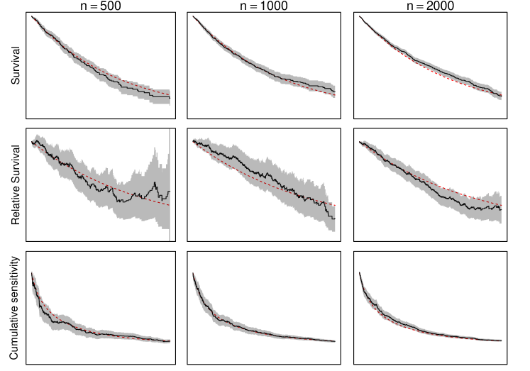
Figure 1. Plugin estimates for selected parameters with population sizes $500,1000,$ and $2000,$ along with 95 % pointwise confidence intervals. Exact parameters is shown in dotted lines.

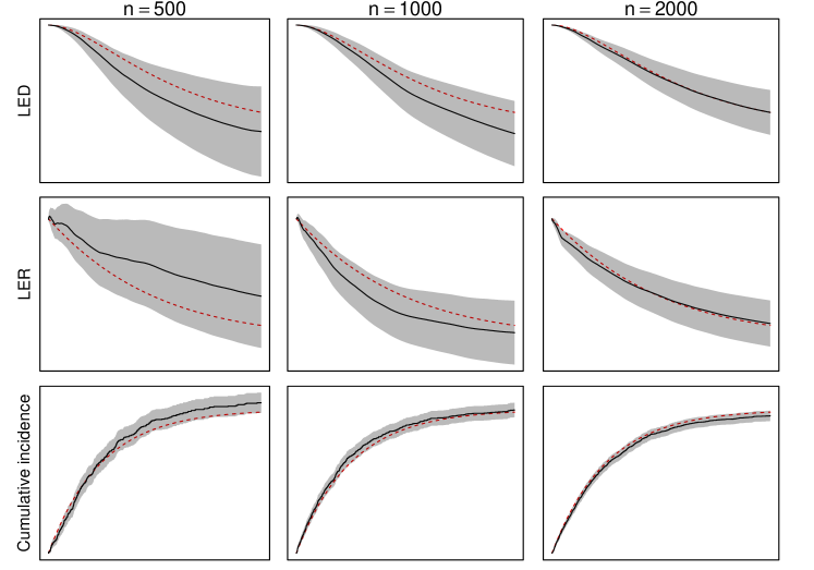
Figure 2. Plugin estimates for selected parameters with population sizes $500,1000,$ and $2000,$ along with 95 % pointwise confidence intervals. Exact parameters is shown in dotted lines. LED and LER are abbreviations for life expectancy difference and life expectancy ratio, respectively.

In the following we write out the plugin estimators for some of the examples we showed in Section 2, using the notation introduced in Definition 1. The most involved variance expressions are moved to the Appendix. We will write $\Delta\tau_{k}:=\tau_{k}-\tau_{k-1}$, and use $e_{i,j}$ to denote matrices with entries equal to zero in all positions apart from the $i$th row and $j$th column where the value is $1$, in order to keep the notation simple. Simulations of selected parameters are displayed in Figures 1 and 2.

4.1. Survival curves

The survival plugin estimator is

$$\hat{S}_{t} =\hat{S}_{\tau_{k-1}}-\hat{S}_{\tau_{k-1}}\Delta\hat{A}_{\tau_{k}},$$

which is nothing but the Kaplan-Meier estimator expressed as a difference equation. The variance plugin estimator is

$$\hat{V}_{t} =\hat{V}_{\tau_{k}-1}-2\hat{V}_{\tau_{k}-1}\Delta\hat{A}_{\tau_{k}}+n\hat{S}_{\tau_{k-1}}(\Delta\hat{A}_{\tau_{k}})^{2}.$$

4.2. Relative survival

The relative survival difference equation is

$$\widehat{RS}_{t}=\widehat{RS}_{\tau_{k-1}}+\begin{pmatrix}-\widehat{RS}_{\tau_{k-1}}&\widehat{RS}_{\tau_{k-1}}\end{pmatrix}\Delta\begin{pmatrix}\hat{A}_{\tau_{k}}^{1}\\ \hat{A}_{\tau_{k}}^{0}\end{pmatrix}.$$

The plugin variance solves

$$\hat{V}_{t}=\hat{V}_{\tau_{k-1}} -2\hat{V}_{\tau_{k-1}}\Delta\hat{A}_{\tau_{k}}^{1}+2\hat{V}_{\tau_{k-1}}\Delta\hat{A}_{\tau_{k}}^{0}$$

$$+n\begin{pmatrix}-\widehat{RS}_{\tau_{k-1}}&\widehat{RS}_{\tau_{k-1}}\end{pmatrix}\Delta\begin{pmatrix}\hat{A}_{\tau_{k}}^{1}\\ \hat{A}_{\tau_{k}}^{0}\end{pmatrix}\Delta\begin{pmatrix}\hat{A}_{\tau_{k}}^{1}&\hat{A}_{\tau_{k}}^{0}\end{pmatrix}\begin{pmatrix}-\widehat{RS}_{\tau_{k-1}}\\ \widehat{RS}_{\tau_{k-1}}\end{pmatrix}.$$

4.3. Mean and restricted mean survival

The restricted mean survival plugin estimator solves

$$\begin{pmatrix}\hat{R}_{t}\\ \hat{S}_{t}\end{pmatrix} =\begin{pmatrix}\hat{R}_{\tau_{k-1}}\\ \hat{S}_{\tau_{k-1}}\end{pmatrix}+\begin{pmatrix}\hat{S}_{\tau_{k-1}}&0\\ 0&-\hat{S}_{\tau_{k-1}}\end{pmatrix}\Delta\begin{pmatrix}\tau_{k}\\ \hat{A}_{\tau_{k}}\end{pmatrix}.$$

The variance expression reads

$$\boldsymbol{\hat{V}}_{t} =\boldsymbol{\hat{V}}_{\tau_{k-1}}+\Big{(}\boldsymbol{\hat{V}}_{\tau_{k-1}}e_{2,1}+e_{1,2}\boldsymbol{\hat{V}}_{\tau_{k-1}}\Big{)}\Delta\tau_{k}$$

$$-\Big{(}\boldsymbol{\hat{V}}_{\tau_{k-1}}e_{2,2}+e_{2,2}\boldsymbol{\hat{V}}_{\tau_{k-1}}\Big{)}\Delta\hat{A}_{\tau_{k}}$$

$$+n\begin{pmatrix}\hat{S}_{\tau_{k-1}}&0\\ 0&-\hat{S}_{\tau_{k-1}}\end{pmatrix}\Delta\begin{pmatrix}0\\ \hat{A}_{\tau_{k}}\end{pmatrix}\Delta\begin{pmatrix}0&\hat{A}_{\tau_{k}}\end{pmatrix}\begin{pmatrix}\hat{S}_{\tau_{k-1}}&0\\ 0&-\hat{S}_{\tau_{k-1}}\end{pmatrix}.$$

4.4. Life expectancy difference and life expectancy ratio

The LED plugin estimator is

$$\begin{pmatrix}\widehat{\text{LED}}_{t}^{12}\\ \hat{S}_{t}^{1}\\ \hat{S}_{t}^{2}\end{pmatrix} =\begin{pmatrix}\widehat{\text{LED}}_{\tau_{k-1}}^{12}\\ \hat{S}_{\tau_{k-1}}^{1}\\ \hat{S}_{\tau_{k-1}}^{2}\end{pmatrix}+\begin{pmatrix}\hat{S}_{\tau_{k-1}}^{1}-\hat{S}_{\tau_{k-1}}^{2}&0&0\\ 0&-\hat{S}_{\tau_{k-1}}^{1}&0\\ 0&0&-\hat{S}_{\tau_{k-1}}^{2}\end{pmatrix}\Delta\begin{pmatrix}\tau_{k}\\ \hat{A}_{\tau_{k}}^{1}\\ \hat{A}_{\tau_{k}}^{2}\end{pmatrix},$$

with variance equation

$$\boldsymbol{\hat{V}}_{t} =\boldsymbol{\hat{V}}_{\tau_{k-1}}+\Big{(}\boldsymbol{\hat{V}}_{\tau_{k-1}}(e_{2,1}-e_{3,1})+(e_{1,2}-e_{1,3})\boldsymbol{\hat{V}}_{\tau_{k-1}}\Big{)}\Delta\tau_{k}$$

$$-\Big{(}\boldsymbol{\hat{V}}_{\tau_{k-1}}e_{2,2}+e_{2,2}\boldsymbol{\hat{V}}_{\tau_{k-1}}\Big{)}\Delta\hat{A}_{\tau_{k}}^{1}$$

$$-\Big{(}\boldsymbol{\hat{V}}_{\tau_{k-1}}e_{3,3}+e_{3,3}\boldsymbol{\hat{V}}_{\tau_{k-1}}\Big{)}\Delta\hat{A}_{\tau_{k}}^{2}$$

$$+nF_{\tau_{k-1}}\Delta\begin{pmatrix}0\\ \hat{A}_{\tau_{k}}^{1}\\ \hat{A}_{\tau_{k}}^{2}\end{pmatrix}\Delta\begin{pmatrix}0&\hat{A}_{\tau_{k}}^{1}&\hat{A}_{\tau_{k}}^{2}\end{pmatrix}F_{\tau_{k-1}}^{\top}.$$

Here $F$ is the LED integrand function, i.e.

$$F_{\tau_{k-1}} =\begin{pmatrix}\hat{S}_{\tau_{k-1}}^{1}-\hat{S}_{\tau_{k-1}}^{2}&0&0\\ 0&\hat{S}_{\tau_{k-1}}^{1}&0\\ 0&0&\hat{S}_{\tau_{k-1}}^{2}\end{pmatrix}.$$

The LER plugin estimator reads

$$\begin{pmatrix}\widehat{\text{LER}}_{t}^{12}\\ \hat{S}_{t}^{1}\\ \hat{S}_{t}^{2}\\ \hat{R}_{t}^{1}\\ \hat{R}_{t}^{2}\end{pmatrix} =\begin{pmatrix}\widehat{\text{LER}}_{\tau_{k-1}}^{12}\\ \hat{S}_{\tau_{k-1}}^{1}\\ \hat{S}_{\tau_{k-1}}^{2}\\ \hat{R}_{\tau_{k-1}}^{1}\\ \hat{R}_{\tau_{k-1}}^{2}\end{pmatrix}+\begin{pmatrix}\frac{\hat{S}_{\tau_{k-1}}^{1}\hat{R}_{\tau_{k-1}}^{2}-\hat{S}_{\tau_{k-1}}^{2}\hat{R}_{\tau_{k-1}}^{1}}{(\hat{R}_{\tau_{k-1}}^{2})^{2}}&0&0\\ 0&-\hat{S}_{\tau_{k-1}}^{1}&0\\ 0&0&-\hat{S}_{\tau_{k-1}}^{2}\\ \hat{S}_{\tau_{k-1}}^{1}&0&0\\ \hat{S}_{\tau_{k-1}}^{2}&0&0\end{pmatrix}\Delta\begin{pmatrix}\tau_{k}\\ \hat{A}_{\tau_{k}}^{1}\\ \hat{A}_{\tau_{k}}^{2}\end{pmatrix}.$$

The variance expression is involved, and can be found in the Appedix.

4.5. Cumulative incidence and competing risks

The plugin estimator for the cumulative incidence example is

$$\begin{pmatrix}\hat{S}_{t}\\ \hat{C}^{1}_{t}\\ \vdots\\ \hat{C}^{m}_{t}\end{pmatrix}=\begin{pmatrix}\hat{S}_{\tau_{k-1}}\\ \hat{C}^{1}_{\tau_{k-1}}\\ \vdots\\ \hat{C}^{m}_{\tau_{k-1}}\end{pmatrix}+\begin{pmatrix}-\hat{S}_{\tau_{k-1}}&-\hat{S}_{\tau_{k-1}}&\dots&-\hat{S}_{\tau_{k-1}}\\ \hat{S}_{\tau_{k-1}}&0&\dots&0\\ 0&\dots&\ddots&\hat{S}_{\tau_{k-1}}\end{pmatrix}\Delta\begin{pmatrix}\hat{A}^{1}_{\tau_{k}}\\ \vdots\\ \hat{A}^{m}_{\tau_{k}}\end{pmatrix},$$

The plugin variance equation is

$$\boldsymbol{\hat{V}}_{t} =\boldsymbol{\hat{V}}_{\tau_{k-1}}+\Big{(}\boldsymbol{\hat{V}}_{\tau_{k-1}}(e_{1,2}-e_{1,1})+(e_{2,1}-e_{1,1})\boldsymbol{\hat{V}}_{\tau_{k-1}}\Big{)}\Delta\hat{A}_{\tau_{k}}^{1}$$

$$+\Big{(}\boldsymbol{\hat{V}}_{\tau_{k-1}}(e_{1,3}-e_{1,1})+(e_{3,1}-e_{1,1})\boldsymbol{\hat{V}}_{\tau_{k-1}}\Big{)}\Delta\hat{A}_{\tau_{k}}^{2}$$

$$\vdots$$

$$+\Big{(}\boldsymbol{\hat{V}}_{\tau_{k-1}}(e_{1,m+1}-e_{1,1})+(e_{m+1,1}-e_{1,1})\boldsymbol{\hat{V}}_{\tau_{k-1}}\Big{)}\Delta\hat{A}_{\tau_{k}}^{m}$$

$$+nF_{\tau_{k-1}}\Delta\begin{pmatrix}\hat{A}_{\tau_{k}}^{1}\\ \vdots\\ \hat{A}_{\tau_{k}}^{m}\end{pmatrix}\Delta\begin{pmatrix}\hat{A}_{\tau_{k}}^{1}&\cdots&\hat{A}_{\tau_{k}}^{m}\end{pmatrix}F_{\tau_{k-1}}^{\top}.$$

4.6. Mean frequency function for recurrent events

We get a plugin estimator equation that reads

$$\begin{pmatrix}\hat{K}_{t}\\ \hat{S}_{t}\end{pmatrix} =\begin{pmatrix}\hat{K}_{\tau_{k-1}}\\ \hat{S}_{\tau_{k-1}}\end{pmatrix}+\begin{pmatrix}\hat{S}_{\tau_{k-1}}&0\\ 0&-\hat{S}_{\tau_{k-1}}\end{pmatrix}\Delta\begin{pmatrix}\hat{A}_{\tau_{k}}^{H}\\ \hat{A}_{\tau_{k}}^{D}\end{pmatrix}.$$

The variance is

$$\boldsymbol{\hat{V}}_{t} =\boldsymbol{\hat{V}}_{\tau_{k-1}}+\Big{(}\boldsymbol{\hat{V}}_{\tau_{k-1}}e_{2,1}+e_{1,2}\boldsymbol{\hat{V}}_{\tau_{k-1}}\Big{)}\Delta\hat{A}_{\tau_{k}}^{H}$$

$$-\Big{(}\boldsymbol{\hat{V}}_{\tau_{k-1}}e_{2,2}+e_{2,2}\boldsymbol{\hat{V}}_{\tau_{k-1}}\Big{)}\Delta\hat{A}_{\tau_{k}}^{D}$$

$$+n\begin{pmatrix}\hat{S}_{\tau_{k-1}}&0\\ 0&-\hat{S}_{\tau_{k-1}}\end{pmatrix}\Delta\begin{pmatrix}\hat{A}_{\tau_{k}}^{H}\\ \hat{A}_{\tau_{k}}^{D}\end{pmatrix}\Delta\begin{pmatrix}\hat{A}_{\tau_{k}}^{H}&\hat{A}_{\tau_{k}}^{D}\end{pmatrix}\begin{pmatrix}\hat{S}_{\tau_{k-1}}&0\\ 0&-\hat{S}_{\tau_{k-1}}\end{pmatrix}.$$

4.7. Cumulative sensitivity and specificity after screening

We have

$$\begin{pmatrix}\hat{U}_{t}\\ \hat{V}_{t}\\ \hat{W}_{t}\\ \hat{X}_{t}\end{pmatrix}=\begin{pmatrix}\hat{U}_{\tau_{k-1}}\\ \hat{V}_{\tau_{k-1}}\\ \hat{W}_{\tau_{k-1}}\\ \hat{X}_{\tau_{k-1}}\end{pmatrix}+\begin{pmatrix}1-\hat{U}_{\tau_{k-1}}&0\\ 0&-\hat{V}_{\tau_{k-1}}\\ \frac{\hat{W}^{2}_{\tau_{k-1}}(1-\hat{V}_{\tau_{k-1}})(1-\hat{U}_{\tau_{k-1}})}{\gamma\hat{U}_{\tau_{k-1}}^{2}}&-\frac{\hat{W}^{2}_{\tau_{k-1}}\hat{V}_{\tau_{k-1}}\hat{U}_{\tau_{k-1}}}{\gamma\hat{U}_{\tau_{k-1}}^{2}}\\ \frac{\gamma\hat{X}_{\tau_{k-1}}^{2}(1-\hat{U}_{\tau_{k-1}})}{\hat{V}_{\tau_{k-1}}}&-\frac{\gamma\hat{X}_{\tau_{k-1}}^{2}(1-\hat{U}_{\tau_{k-1}})}{\hat{V}_{\tau_{k-1}}}\end{pmatrix}\Delta\begin{pmatrix}\hat{A}^{1}_{\tau_{k}}\\ \hat{A}^{0}_{\tau_{k}}\end{pmatrix},$$

The variance expression can be found in the Appendix.

5. Performance

5.1. Convergence

Our convergence assessment involves two steps. In step one we find close approximations to the parameters, using the notation $\tilde{X}$. In step two we calculate plugin estimators for a range of sample sizes. We then check how fast the plugin estimators converge to $\tilde{X}$ as the sample size increases.

For performing step one we have developed code that generates survival data for given input hazards. Using the hazards we can calculate $\tilde{X}$ to desired precision. For instance, knowing the hazard $\alpha$ we can obtain the survival $e^{-\int\alpha_{s}ds}$ by numerical integration.

For performing step two we simulate data, enabling us to estimate cumulative hazards, and therefore parameters specified by (9). This step is performed for a range of sample sizes. For each sample size $n$ we simulate $k$ populations, such that we obtain plugin estimates $\hat{X}^{n,j}$, for $j=1,\cdots,k$. We check convergence using the following $L^{2}$ criterion:

(20) $$L(n) =\frac{1}{k}\sum_{j=1}^{k}\int_{0}^{\mathcal{T}}(\tilde{X}_{s}-\hat{X}_{s}^{n,j})^{2}ds.$$

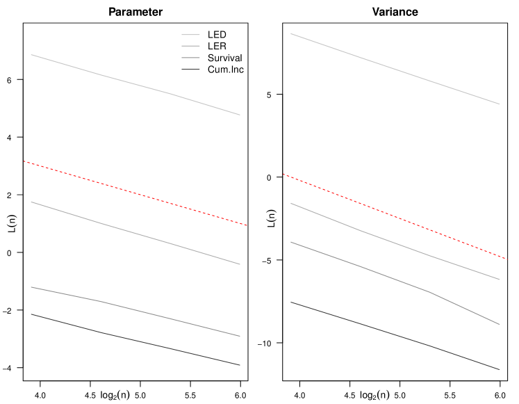
Figure 3. Convergence of selected plugin estimators; parameter to the left and variances to the right. We used dashed lines indicating convergence order $1$ in the left panel and $2.3$ in the right panel. LED and LER are abbreviations for life expectancy difference and life expectancy ratio, respectively.

For assessing convergence of the plugin variance estimators we first obtain a variance estimate from a large bootstrap sample. As in step two above, we simulate data and obtain $k$ plugin variance estimates for a range of sample sizes $n$. In this way the same criterion (20) can be used. Convergence plots are shown in Figure 3.

Figure 3 suggests that the LED estimator performs worse than the other estimators. This happens because the variance depends on the time scale, since we are approximating Lebesgue integrals. The LER plugin variance also depends on the time scale, but here the time contribution is smaller.

5.2. Coverage

To estimate coverage we first obtain close approximations to the parameters, $\tilde{X}$, as described in step one in Section 5.1. Next, we simulated data to calculate plugin estimates, which were used to obtain confidence intervals. This step is repeated until we have a large collection of confidence intervals. At time $t$, a Bernoulli trial decides whether a confidence interval covers $\tilde{X}_{t}$. We estimate the expected coverage at time $t$ by this Bernoulli probability, i.e. by the average number of confidence intervals that cover $\tilde{X}_{t}$.

We calculate coverage for two scenarios; constant hazards, and linear (crossing) hazards over a time period $[0,\mathcal{T}]$. We selected linear hazards that were large initially but linearly decreasing, or small initially but linearly increasing, such that they crossed each other at the halfway point $\mathcal{T}/2$.

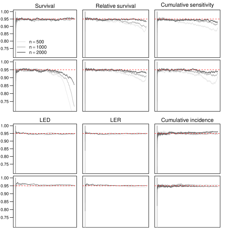
Figure 4. Estimated mean coverage for selected parameters simulated with constant(upper panel) and linearly crossing(lower panel) hazards. The dotted line indicates the confidence level. LED and LER are abbreviations for life expectancy difference and life expectancy ratio, respectively.

Coverage is shown in Figure 4, suggesting that the coverage drops below the confidence level in some scenarios. This behavior is due to the plugin variance estimators. The Survival plugin variance, for instance, will drop drastically if there are events when few people are at risk, causing the Survival confidence interval to be narrow thereafter. Incidentally, the Greenwood estimator would give similar performance, since it is small whenever the Kaplan–Meier curve is small.

Overall the plugin estimators behave satisfactory, not only when the hazards are constant but also when the hazards are linearly crossing.

6. Software

R software for calculating plugin estimators, illustrated on simulated data examples, can be found on

https://github.com/palryalen/transform.hazards. For questions or comments regarding the shared code, contact p.c.ryalen@medisin.uio.no.

7. Funding

The authors were all supported by the research grant NFR239956/F20 - Analyzing clinical health registries: Improved software and mathematics of identifiability.

Appendix: Proofs

7.1. Proof of Lemma 1

Proof.

We start by proving that $\{\boldsymbol{M}^{(n)}\}_{n}$ is P-UT. Suppose that $\boldsymbol{H}$ is predictable, matrix-valued and such that $\operatorname{Tr}(\boldsymbol{H}_{s}^{\intercal}\boldsymbol{H}_{s})$ bounded by $1$. Note that for every optional stopping time $\tau$:

$$E\big{[}\big{|}\int_{0}^{\tau}\boldsymbol{H}_{s}d\boldsymbol{M}_{s}^{(n)}\big{|}_{2}^{2}\big{]}=E\big{[}\text{Tr}\int_{0}^{\tau}\boldsymbol{H}_{s}d\boldsymbol{M}_{s}^{(n)}\big{(}\int_{0}^{\tau}\boldsymbol{H}_{s}d\boldsymbol{M}_{s}^{(n)}\big{)}^{\intercal}\big{]}$$

$$= E\big{[}\text{Tr}\int_{0}^{\tau}\boldsymbol{H}_{s}d\langle\boldsymbol{M}^{(n)}\rangle_{s}\boldsymbol{H}_{s}^{\intercal}\big{]}\leq E\big{[}\int_{0}^{\tau}\operatorname{Tr}(\boldsymbol{H}_{s}^{\intercal}\boldsymbol{H}_{s})d\text{Tr}\langle\boldsymbol{M}^{(n)}\rangle_{s}\big{]}$$

$$\leq E\big{[}\int_{0}^{\tau}d\text{Tr}\langle\boldsymbol{M}^{(n)}\rangle_{s}\big{]}=E\big{[}\text{Tr}\langle\boldsymbol{M}^{(n)}\rangle_{\tau}\big{]}.$$

The Lenglart-inequality [25, I-3.31] therefore implies that $\{\boldsymbol{M}^{(n)}\}_{n}$ is P-UT.

For the first term $\ref{eq:tightRho})$ we have that $\text{Var}(\int_{0}^{\cdot}\boldsymbol{\rho}_{s}^{(n)}ds)_{t}=\int_{0}^{t}|\boldsymbol{\rho}_{s}^{(n)}|_{1}ds$ is uniformly tight for every $t$, which by [25, VI 6.12] implies that $\{\boldsymbol{\rho}^{(n)}\}_{n}$ is P-UT. Finally, the claim follows since $\{\boldsymbol{Z}^{(n)}\}_{n}$ is the sum of two sequences that are P-UT.

∎

7.2. Proof of Theorem 1

Proof.

We are given a series of SDEs that converges to an SDE (actually just an ODE), and want to assure that this means that their solutions also converge to the solution of the limit equation. This is a claim about stability of stochastic differential equations. We want to prove our claim with an application of [25, Theorem IX.6.9]. Translated into our situation, it says that if $(\boldsymbol{\hat{X}}_{0}^{(n)},\boldsymbol{\hat{A}}^{(n)})$ converges in law to $(\boldsymbol{X}_{0},\boldsymbol{A})$ and the series $\{\boldsymbol{\hat{A}}^{(n)}\}_{n}$ is predictably uniformly tight (P-UT), then $(\boldsymbol{\hat{X}}_{0}^{(n)},\boldsymbol{\hat{A}}^{(n)},\boldsymbol{\hat{X}}^{(n)})$ also converges in law to $(\boldsymbol{X}_{0},\boldsymbol{A},\boldsymbol{X})$.

Moreover, [25, VI.3.33] ensures convergence of $(\boldsymbol{\hat{X}}_{0}^{(n)},\boldsymbol{\hat{A}}^{(n)})$. The advertised result follows from the continuity of the projection mapping.∎

7.3. Proof of Theorem 2

Proof.

We will first prove that $\{\boldsymbol{\hat{Z}}^{(n)}\}$ converges in law to $\boldsymbol{Z}$ by another application of the stability result for SDEs found in [25, Theorem IX.6.9]. Then we will prove that the covariance of $\boldsymbol{Z}$ is given by the ODE (17). Finally, we will apply the SDE-stability result once more to see that the solutions of the SDE (15) converge in law to the covariance of $\boldsymbol{Z}$.

To prove that $\{\boldsymbol{Z}^{(n)}\}$ converges in law, we start with the following approximation of the derivative of $F_{j}$ in the direction $z$:

(21) $$DF^{n}_{j}(x,z):=\sqrt{n}\big{(}F_{j}(x+n^{-1/2}z)-F_{j}(x)\big{)},$$

let $DF^{n}(x,z):=\begin{pmatrix}DF^{n}_{1}(x,z),&\dots&,DF^{n}_{l}(x,z)\end{pmatrix}$ and note that we have

$$\lim_{n}DF^{n}_{j}(x,z)=\nabla F_{j}(x)z.$$

Now,

$$\boldsymbol{Z}_{t}^{(n)}=\sqrt{n}\big{(}\boldsymbol{\hat{X}}_{t}^{(n)}-\boldsymbol{X}_{t}\big{)}$$

$$= \boldsymbol{Z}_{0}^{(n)}+\sum_{j=1}^{k}\int_{0}^{t}\sqrt{n}\bigg{(}F_{j}(\boldsymbol{\hat{X}}_{s-}^{(n)})-F_{j}(\boldsymbol{X}_{s})\bigg{)}d{\hat{A}}_{s}^{j(n)}+\int_{0}^{t}F(\boldsymbol{X}_{s})d\boldsymbol{W}^{(n)}_{s}$$

$$= \boldsymbol{Z}_{0}^{(n)}+\sum_{j=1}^{k}\int_{0}^{t}DF^{n}_{j}(\boldsymbol{X}_{s},\boldsymbol{Z}^{(n)}_{s-})d\hat{A}^{j(n)}_{s}+\int_{0}^{t}F(\boldsymbol{X}_{s})d\boldsymbol{W}^{(n)}_{s}$$

$$= \boldsymbol{Z}_{0}^{(n)}+\int_{0}^{t}DF^{n}(\boldsymbol{X}_{s},\boldsymbol{Z}^{(n)}_{s-})d\boldsymbol{\hat{A}}^{(n)}_{s}+\int_{0}^{t}F(\boldsymbol{X}_{s})d\boldsymbol{W}^{(n)}_{s}.$$

Now [25, Theorem VI.6.22] implies that $\{\boldsymbol{Z}_{0}^{(n)}+\int_{0}^{\cdot}F(\boldsymbol{X}_{s})d\boldsymbol{W}^{(n)}_{s}\}_{n}$ converges is law to $\boldsymbol{Z}_{0}+\int_{0}^{\cdot}F(\boldsymbol{X}_{s})d\boldsymbol{W}_{s}$, and since $\boldsymbol{A}$ is continuous, [25, Corollary VI.3.33] implies that $\{(\boldsymbol{Z}_{0}^{(n)}+\int_{0}^{\cdot}F(\boldsymbol{X}_{s})d\boldsymbol{W}^{(n)}_{s},\boldsymbol{\hat{A}}^{(n)})\}_{n}$ converges in law to $(\boldsymbol{Z}_{0}+\int_{0}^{\cdot}F(\boldsymbol{X}_{s})d\boldsymbol{W}_{s},\boldsymbol{A})$.

Since $F$ has bounded and continuous first and second derivatives, a calculus argument shows that $\{DF^{n}\}_{n}$ have uniformly bounded Lipschitz constants by the Lipcschitz constant of $F$. This enables us to apply the stability result for SDEs found in [25, Theorem IX.6.9] again. It says that since $\{\boldsymbol{\hat{A}}^{(n)}\}_{n}$ is predictably uniformly tight, we also have that $\{(\boldsymbol{Z}_{0}^{(n)}+\int_{0}^{\cdot}F(\boldsymbol{X}_{s})d\boldsymbol{W}^{(n)}_{s},\boldsymbol{\hat{A}}^{(n)},\boldsymbol{Z}^{(n)})\}_{n}$ converges in law to $(\boldsymbol{Z}_{0}+\int_{0}^{\cdot}F(\boldsymbol{X}_{s})d\boldsymbol{W}_{s},\boldsymbol{A},\boldsymbol{Z})$.

To see that the covariance of $\boldsymbol{Z}$ is given by the ODE (17), we note that $[\boldsymbol{W}]$ is deterministic since $\boldsymbol{W}$ is a continuous Gaussian martingale with independent increments, and that

$$E\big{[}\boldsymbol{Z}_{t}\boldsymbol{Z}_{t}^{\intercal}\big{]}= E\big{[}\boldsymbol{Z}_{0}\boldsymbol{Z}_{0}^{\intercal}\big{]}+E\bigg{[}\int_{0}^{t}\boldsymbol{Z}_{s-}d\boldsymbol{Z}_{s}^{\intercal}\bigg{]}+E\bigg{[}\int_{0}^{t}d\boldsymbol{Z}_{s}\boldsymbol{Z}_{s-}^{\intercal}\bigg{]}+E\big{[}[\boldsymbol{Z},\boldsymbol{Z}]_{t}\big{]}$$

$$= E\big{[}\boldsymbol{Z}_{0}\boldsymbol{Z}_{0}^{\intercal}\big{]}+E\bigg{[}\sum_{j=1}^{k}\int_{0}^{t}\boldsymbol{Z}_{s-}dA_{s}^{j}\boldsymbol{Z}_{s-}^{\intercal}\nabla F_{j}(\boldsymbol{X}_{s})^{\intercal}\bigg{]}$$

$$+E\bigg{[}\sum_{j=1}^{k}\int_{0}^{t}\nabla F_{j}(\boldsymbol{X}_{s})\boldsymbol{Z}_{s-}dA^{j}_{s}\boldsymbol{Z}_{s-}^{\intercal}\bigg{]}$$

$$+E\bigg{[}\int_{0}^{t}F(\boldsymbol{X}_{s-})d[\boldsymbol{W}]_{s}F(\boldsymbol{X}_{s-})^{\intercal}\bigg{]}$$

$$= E\big{[}\boldsymbol{Z}_{0}\boldsymbol{Z}_{0}^{\intercal}\big{]}+\sum_{j=1}^{k}\int_{0}^{t}E\big{[}\boldsymbol{Z}_{s-}\boldsymbol{Z}_{s-}^{\intercal}\big{]}\nabla F_{j}(\boldsymbol{X}_{s})^{\intercal}dA_{s}^{j}$$

$$+\sum_{j=1}^{k}\int_{0}^{t}\nabla F_{j}(\boldsymbol{X}_{s})E\big{[}\boldsymbol{Z}_{s-}\boldsymbol{Z}_{s-}^{\intercal}\big{]}dA^{j}$$

$$+\int_{0}^{t}F(\boldsymbol{X}_{s-})d[\boldsymbol{W}]_{s}F(\boldsymbol{X}_{s-})^{\intercal}.$$

We now show that the solutions of the SDE (15) converge in law to the covariance of $\boldsymbol{Z}$. We first note that [25, Theorem VI.6.26] implies that $\{[\boldsymbol{W}^{(n)}]\}_{n}$ converges in law to $[\boldsymbol{W}]$ since $\{\boldsymbol{W}^{(n)}\}_{n}$ is predictably uniformly tight. Moreover, since $\boldsymbol{A}$ is continuous, [25, Corollary VI 3.33] implies that $\{(\boldsymbol{\hat{A}}^{(n)},[\boldsymbol{W}^{(n)}])\}_{n}$ converges in law to $(\boldsymbol{A},[\boldsymbol{W}])$. If this sequence was predictably uniformly tight, then we could apply [25, Theorem IX.6.9] one more time to ensure that the solutions of the SDEs (15) converge in law to $\boldsymbol{V}$.

Finally, note that $\{(\boldsymbol{\hat{A}}^{(n)},[\boldsymbol{W}^{(n)}])\}_{n}$ is P-UT since both $\{\boldsymbol{\hat{A}}^{(n)}\}_{n}$ and $\{[\boldsymbol{W}^{(n)}]\}_{n}$ are P-UT.

∎

7.4. Proof of Proposition 1

Proof.

It is well known that $\boldsymbol{W}^{(n)}:=\sqrt{n}(\boldsymbol{A}^{(n)}-\boldsymbol{A})$ converges weakly to a Gaussian process with independent increments, see [14]. To see that $\{\boldsymbol{W}^{(n)}\}_{n}$ is P-UT, let

(22) $$\boldsymbol{\Gamma}^{(n)}_{t}:=\frac{\boldsymbol{U}^{(n)\intercal}_{t-}\boldsymbol{Y}^{(n)}_{t}\boldsymbol{U}_{t-}^{(n)}}{n},$$

and note that

$$\operatorname{Tr}\langle\boldsymbol{W}^{(n)}\rangle_{\mathcal{T}}= \int_{0}^{\mathcal{T}}\operatorname{Tr}\big{(}\boldsymbol{\Gamma}^{(n)-1}_{t}\frac{\boldsymbol{U}^{(n)\intercal}_{t-}\boldsymbol{\lambda}_{t}^{(n)}\boldsymbol{Y}^{(n)}_{t}\boldsymbol{U}_{t-}^{(n)}}{n}\boldsymbol{\Gamma}^{(n)-1}_{t}\big{)}dt.$$

From the submultiplicativity of the trace norm we have

$$\operatorname{Tr}\big{(}\boldsymbol{\Gamma}^{(n)-1}_{t}\frac{\boldsymbol{U}^{(n)\intercal}_{t-}\boldsymbol{\lambda}_{t}^{(n)}\boldsymbol{Y}^{(n)}_{t}\boldsymbol{U}_{t-}^{(n)}}{n}\boldsymbol{\Gamma}^{(n)-1}_{t}\big{)}$$

$$\leq \operatorname{Tr}\big{(}\boldsymbol{\Gamma}^{(n)-1}_{t}\big{)}\operatorname{Tr}\bigg{(}\frac{\boldsymbol{U}^{(n)\intercal}_{t-}\boldsymbol{\lambda}_{t}^{(n)}\boldsymbol{Y}^{(n)}_{t}\boldsymbol{U}_{t-}^{(n)}}{n}\bigg{)}\operatorname{Tr}\big{(}\boldsymbol{\Gamma}^{(n)-1}_{t}\big{)}.$$

On the other hand, we have that

(23) $$\operatorname{Tr}\bigg{(}\frac{\boldsymbol{U}^{(n)\intercal}_{t-}\boldsymbol{\lambda}_{t}^{(n)}\boldsymbol{Y}^{(n)}_{t}\boldsymbol{U}_{t-}^{(n)}}{n}\bigg{)}=\frac{1}{n}\sum_{k,i}(U_{t-}^{k,i})^{2}Y_{t}^{i}\lambda_{t}^{i},$$

and $E_{P}[\sup_{t\leq\mathcal{T}}|(U_{t-}^{k,i})^{2}Y_{t}^{i}\lambda^{i}_{t}|]<\infty$, so Markovs inequality implies that

(24) $$\lim_{J}\inf_{n}P\bigg{(}\operatorname{Tr}\Big{(}\frac{\boldsymbol{U}^{(n)\intercal}_{t-}\boldsymbol{\lambda}_{t}^{(n)}\boldsymbol{Y}^{(n)}_{t}\boldsymbol{U}_{t-}^{(n)}}{n}\Big{)}\geq J\bigg{)}=0.$$

Finally, [14, Proposition II.5.3] implies that (8) of Lemma 1 is satisfied.

Note that $\{\boldsymbol{A}^{(n)}\}_{n}$ is P-UT since $\boldsymbol{A}^{(n)}=\frac{1}{\sqrt{n}}\boldsymbol{W}^{(n)}+\boldsymbol{A}_{t}$. To see that $\{[\boldsymbol{W}^{(n)}]\}_{n}$ is P-UT, note that we have already seen that the compensator of $[\boldsymbol{W}^{(n)}]$, $\langle\boldsymbol{W}^{(n)}\rangle$, satisfies (8) of Lemma 1. Moreover, note that

$$\operatorname{Tr}\big{(}\langle[\boldsymbol{W}^{(n)}]-\langle\boldsymbol{W}^{(n)}\rangle\rangle_{\mathcal{T}}\big{)}=\operatorname{Tr}\big{(}\langle\boldsymbol{W}^{(n)}\rangle_{\mathcal{T}}\big{)},$$

so $\eqref{eq:PUTMart}$ of Lemma 1 is satisfied for $\{[\boldsymbol{W}^{(n)}]-\langle\boldsymbol{W}^{(n)}\rangle\}_{n}$ as well, which therefore implies that $\{[\boldsymbol{W}^{(n)}]\}_{n}$ is P-UT.

∎

Appendix: Other plugin variance expressions

Variance for LER

Here, the plugin variance reads

$$\boldsymbol{\hat{V}}_{t} =\boldsymbol{\hat{V}}_{\tau_{k-1}}+\Big{(}\boldsymbol{\hat{V}}_{\tau_{k-1}}G_{\tau_{k-1}}^{\top}+G_{\tau_{k-1}}\boldsymbol{\hat{V}}_{\tau_{k-1}}\Big{)}\Delta\tau_{k}$$

$$-\Big{(}\boldsymbol{\hat{V}}_{\tau_{k-1}}e_{2,2}+e_{2,2}\boldsymbol{\hat{V}}_{\tau_{k-1}}\Big{)}\Delta\hat{A}_{\tau_{k}}^{1}$$

$$-\Big{(}\boldsymbol{\hat{V}}_{\tau_{k-1}}e_{3,3}+e_{3,3}\boldsymbol{\hat{V}}_{\tau_{k-1}}\Big{)}\Delta\hat{A}_{\tau_{k}}^{2}$$

$$+nF_{\tau_{k-1}}\Delta\begin{pmatrix}0\\ \hat{A}_{\tau_{k}}^{1}\\ \hat{A}_{\tau_{k}}^{2}\end{pmatrix}\Delta\begin{pmatrix}0&\hat{A}_{\tau_{k}}^{1}&\hat{A}_{\tau_{k}}^{2}\end{pmatrix}F_{\tau_{k-1}}^{\top},$$

where $G$ and $F$ is given by

$$G_{\tau_{k-1}} =\begin{pmatrix}0&\frac{1}{\hat{R}_{\tau_{k-1}}^{2}}&-\frac{\hat{R}_{\tau_{k-1}}^{1}}{(\hat{R}_{\tau_{k-1}}^{2})^{2}}&-\frac{\hat{S}_{\tau_{k-1}}^{2}}{(\hat{R}_{\tau_{k-1}}^{2})^{2}}&\frac{2\hat{S}_{\tau_{k-1}}^{2}\hat{R}_{\tau_{k-1}}^{1}-\hat{S}_{\tau_{k-1}}^{1}\hat{R}_{\tau_{k-1}}^{2}}{(\hat{R}_{\tau_{k-1}}^{2})^{3}}\\ 0&0&0&0&0\\ 0&0&0&0&0\\ 0&1&0&0&0\\ 0&0&1&0&0\end{pmatrix}$$

$$F_{\tau_{k-1}} =\begin{pmatrix}\frac{\hat{S}_{\tau_{k-1}}^{1}\hat{R}_{\tau_{k-1}}^{2}-\hat{S}_{\tau_{k-1}}^{2}\hat{R}_{\tau_{k-1}}^{1}}{(\hat{R}_{\tau_{k-1}}^{2})^{2}}&0&0\\ 0&-\hat{S}_{\tau_{k-1}}^{1}&0\\ 0&0&-\hat{S}_{\tau_{k-1}}^{2}\\ \hat{S}_{\tau_{k-1}}^{1}&0&0\\ \hat{S}_{\tau_{k-1}}^{2}&0&0\end{pmatrix}$$

Variance for cumulative sensitivity and specificity

In this case the plugin variance is

$$\boldsymbol{\hat{V}}_{t} =\boldsymbol{\hat{V}}_{\tau_{k-1}}+\Big{(}\boldsymbol{\hat{V}}_{\tau_{k-1}}G_{\tau_{k-1}}^{1\top}+G_{\tau_{k-1}}^{1}\boldsymbol{\hat{V}}_{\tau_{k-1}}\Big{)}\Delta\hat{A}_{\tau_{k}}^{1}$$

$$+\Big{(}\boldsymbol{\hat{V}}_{\tau_{k-1}}G_{\tau_{k-1}}^{2\top}+G_{\tau_{k-1}}^{2}\boldsymbol{\hat{V}}_{\tau_{k-1}}\Big{)}\hat{A}_{\tau_{k}}^{0}$$

$$+nF_{\tau_{k-1}}\Delta\begin{pmatrix}\hat{A}_{\tau_{k}}^{1}\\ \hat{A}_{\tau_{k}}^{0}\end{pmatrix}\Delta\begin{pmatrix}\hat{A}_{\tau_{k}}^{1}&\hat{A}_{\tau_{k}}^{0}\end{pmatrix}F_{\tau_{k-1}}^{\top}.$$

Here we have defined

$$G^{1}_{\tau_{k-1}} =\begin{pmatrix}-1&0&0&0\\ 0&0&0&0\\ \frac{\hat{W}_{\tau_{k-1}}^{2}(1-\hat{V}_{\tau_{k-1}})(\hat{U}_{\tau_{k-1}}-2)}{\gamma\hat{U}^{3}_{\tau_{k-1}}}&\frac{\hat{W}^{2}_{\tau_{k-1}}(\hat{U}_{\tau_{k-1}}-1)}{\gamma\hat{U}^{2}_{\tau_{k-1}}}&\frac{2\hat{W}_{\tau_{k-1}}(1-\hat{U}_{\tau_{k-1}})(1-\hat{V}_{\tau_{k-1}})}{\gamma\hat{U}^{2}_{\tau_{k-1}}}&0\\ -\frac{\gamma\hat{X}^{2}_{\tau_{k-1}}}{\hat{V}_{\tau_{k-1}}}&-\frac{\gamma\hat{X}^{2}_{\tau_{k-1}}(1-\hat{U}_{\tau_{k-1}})}{\hat{V}^{2}_{\tau_{k-1}}}&0&\frac{2\gamma\hat{X}_{\tau_{k-1}}(1-\hat{U}_{\tau_{k-1}})}{\hat{V}_{\tau_{k-1}}}\end{pmatrix},$$

$$G_{\tau_{k-1}}^{2} =\begin{pmatrix}0&0&0&0\\ 0&-1&0&0\\ \frac{\hat{W}_{\tau_{k-1}}^{2}\hat{V}_{\tau_{k-1}}}{\gamma\hat{U}^{2}_{\tau_{k-1}}}&-\frac{\hat{W}_{\tau_{k-1}}}{\gamma\hat{U}_{\tau_{k-1}}}&-\frac{2\hat{W}_{\tau_{k-1}}\hat{V}_{\tau_{k-1}}}{\gamma\hat{U}_{\tau_{k-1}}}&0\\ \frac{\gamma\hat{X}^{2}_{\tau_{k-1}}}{\hat{V}_{\tau_{k-1}}}&\frac{\gamma\hat{X}^{2}_{\tau_{k-1}}(1-\hat{U}_{\tau_{k-1}})}{\hat{V}^{2}_{\tau_{k-1}}}&0&-\frac{2\gamma\hat{X}_{\tau_{k-1}}(1-\hat{U}_{\tau_{k-1}})}{\hat{V}_{\tau_{k-1}}}\end{pmatrix},$$

$$F_{\tau_{k-1}} =\begin{pmatrix}1-\hat{U}_{\tau_{k-1}}&0\\ 0&-\hat{V}_{\tau_{k-1}}\\ \frac{\hat{W}^{2}_{\tau_{k-1}}(1-\hat{V}_{\tau_{k-1}})(1-\hat{U}_{\tau_{k-1}})}{\gamma\hat{U}_{\tau_{k-1}}^{2}}&-\frac{\hat{W}^{2}_{\tau_{k-1}}\hat{V}_{\tau_{k-1}}\hat{U}_{\tau_{k-1}}}{\gamma\hat{U}_{\tau_{k-1}}^{2}}\\ \frac{\gamma\hat{X}_{\tau_{k-1}}^{2}(1-\hat{U}_{\tau_{k-1}})}{\hat{V}_{\tau_{k-1}}}&-\frac{\gamma\hat{X}_{\tau_{k-1}}^{2}(1-\hat{U}_{\tau_{k-1}})}{\hat{V}_{\tau_{k-1}}}\end{pmatrix}.$$

References

- [1] O. O. Aalen, R. J. Cook, and K. Røysland, “Does cox analysis of a randomized survival study yield a causal treatment effect?,” Lifetime data analysis, vol. 21, no. 4, pp. 579–593, 2015.
- [2] J. Robins and S. Greenland, “The probability of causation under a stochastic model for individual risk,” Biometrics, pp. 1125–1138, 1989.
- [3] S. Greenland, “Absence of confounding does not correspond to collapsibility of the rate ratio or rate difference,” Epidemiology, pp. 498–501, 1996.
- [4] M. J. Stensrud, M. Valberg, K. Røysland, and O. O. Aalen, “Exploring selection bias by causal frailty models: The magnitude matters,” Epidemiology, vol. 28, no. 3, pp. 379–386, 2017.
- [5] O. Aalen, O. Borgan, and H. Gjessing, Survival and event history analysis: a process point of view. Springer Science & Business Media, 2008.
- [6] M. A. Hernán, “The hazards of hazard ratios,” Epidemiology (Cambridge, Mass.), vol. 21, no. 1, p. 13, 2010.
- [7] M. A. Hernán and J. M. Robins, Causal inference. CRC Boca Raton, FL:, 2017.
- [8] T. Martinussen, S. Vansteelandt, M. Gerster, and J. v. B. Hjelmborg, “Estimation of direct effects for survival data by using the aalen additive hazards model,” Journal of the Royal Statistical Society: Series B (Statistical Methodology), vol. 73, no. 5, pp. 773–788, 2011.
- [9] T. Lange and J. V. Hansen, “Direct and indirect effects in a survival context,” Epidemiology, vol. 22, no. 4, pp. 575–581, 2011.
- [10] S. Strohmaier, K. Røysland, R. Hoff, Ø. Borgan, T. R. Pedersen, and O. O. Aalen, “Dynamic path analysis–a useful tool to investigate mediation processes in clinical survival trials,” Statistics in medicine, vol. 34, no. 29, pp. 3866–3887, 2015.
- [11] T. Martinussen and S. Vansteelandt, “On collapsibility and confounding bias in cox and aalen regression models,” Lifetime data analysis, vol. 19, no. 3, pp. 279–296, 2013.
- [12] M. J. Bradburn, T. G. Clark, S. Love, and D. Altman, “Survival analysis part ii: multivariate data analysis–an introduction to concepts and methods,” British journal of cancer, vol. 89, no. 3, p. 431, 2003.
- [13] R. D. Gill, J. A. Wellner, and J. Præstgaard, “Non-and semi-parametric maximum likelihood estimators and the von mises method (part 1)[with discussion and reply],” Scandinavian Journal of Statistics, pp. 97–128, 1989.
- [14] P. K. Andersen, Ø. Borgan, R. D. Gill, and N. Keiding, Statistical models based on counting processes. Springer Series in Statistics, New York: Springer-Verlag, 1993.
- [15] A. W. Van der Vaart, Asymptotic statistics, vol. 3. Cambridge university press, 1998.
- [16] M. P. Perme, J. Stare, and J. Estève, “On estimation in relative survival,” Biometrics, vol. 68, no. 1, pp. 113–120, 2012.
- [17] P. Royston and M. K. Parmar, “The use of restricted mean survival time to estimate the treatment effect in randomized clinical trials when the proportional hazards assumption is in doubt,” Statistics in medicine, vol. 30, no. 19, pp. 2409–2421, 2011.
- [18] P. Royston and M. K. Parmar, “Restricted mean survival time: an alternative to the hazard ratio for the design and analysis of randomized trials with a time-to-event outcome,” BMC medical research methodology, vol. 13, no. 1, p. 152, 2013.
- [19] L. Trinquart, J. Jacot, S. C. Conner, and R. Porcher, “Comparison of treatment effects measured by the hazard ratio and by the ratio of restricted mean survival times in oncology randomized controlled trials,” Journal of Clinical Oncology, vol. 34, no. 15, pp. 1813–1819, 2016.
- [20] H.-M. Dehbi, P. Royston, and A. Hackshaw, “Life expectancy difference and life expectancy ratio: two measures of treatment effects in randomised trials with non-proportional hazards,” BMJ, vol. 357, p. j2250, 2017.
- [21] P. K. Andersen, R. B. Geskus, T. de Witte, and H. Putter, “Competing risks in epidemiology: possibilities and pitfalls,” International journal of epidemiology, vol. 41, no. 3, pp. 861–870, 2012.
- [22] P. K. Andersen, S. Z. Abildstrom, and S. Rosthøj, “Competing risks as a multi-state model,” Statistical methods in medical research, vol. 11, no. 2, pp. 203–215, 2002.
- [23] D. Ghosh and D. Lin, “Nonparametric analysis of recurrent events and death,” Biometrics, 2000.
- [24] M. Nygård, K. Røysland, S. Campbell, and J. Dillner, “Comparative effectiveness study on human papillomavirus detection methods used in the cervical cancer screening programme,” BMJ open, vol. 4, no. 1, p. e003460, 2014.
- [25] J. Jacod and A. N. Shiryaev, Limit theorems for stochastic processes, vol. 288 of Grundlehren der Mathematischen Wissenschaften [Fundamental Principles of Mathematical Sciences]. Berlin: Springer-Verlag, second ed., 2003.