Virtual Elements for a shear-deflection formulation of Reissner-Mindlin plates

Abstract.

We present a virtual element method for the Reissner–Mindlin plate bending problem which uses shear strain and deflection as discrete variables without the need of any reduction operator. The proposed method is conforming in $[H^{1}(\Omega)]^{2}\times H^{2}(\Omega)$ and has the advantages of using general polygonal meshes and yielding a direct approximation of the shear strains. The rotations are then obtained by a simple postprocess from the shear strain and deflection. We prove convergence estimates with involved constants that are uniform in the thickness $t$ of the plate. Finally, we report numerical experiments which allow us to assess the performance of the method.

1. Introduction

The Virtual Element Method (VEM), introduced in [8, 9], is a recent generalization of the Finite Element Method which is characterized by the capability of dealing with very general polygonal/polyhedral meshes. The interest in numerical methods that can make use of general polytopal meshes has recently undergone a significant growth in the mathematical and engineering literature; among the large number of papers on this subject, we cite as a minimal sample [4, 8, 11, 26, 31, 42, 45, 46].

Indeed, polytopal meshes can be very useful for a wide range of reasons, including meshing of the domain (such as cracks) and data (such as inclusions) features, automatic use of hanging nodes, use of moving meshes, adaptivity. Moreover, the VEM presents the advantage to easily implement highly regular discrete spaces. Indeed, by avoiding the explicit construction of the local basis functions, the VEM can easily handle general polygons/polyhedrons without complex integrations on the element (see [9] for details on the coding aspects of the method). The Virtual Element Method has been applied successfully in a large range of problems, see for instance [1, 2, 7, 8, 9, 12, 15, 16, 17, 20, 23, 25, 28, 35, 39, 40, 41, 47, 48].

The Reissner–Mindlin plate bending problem is used to approximate the deformation of a thin or moderately thick elastic plate. Nowadays, it is very well understood that the discretization of this problem poses difficulties due to the so called locking phenomenon when the thickness $t$ is small with respect to the other dimensions of the plate. Nevertheless, adopting for instance a reduced integration or a mixed interpolation technique, this phenomenon can be avoided. Indeed, several families of methods have been rigorously shown to be free from locking and optimally convergent. We mention [34, 37] for a thorough description and further references.

Recently, a new approach to solve the Reissner–Mindlin bending problem has been presented in [10] by Beirão da Veiga et al. (see also [33, 36]). In this case a variational formulation of the plate bending problem is written in terms of shear strain and deflection with the advantage that the “shear locking phenomenon” is avoided. A discretization of the problem by Isogeometric Analysis is proposed. Under some regularity assumptions on the exact solution, optimal error estimates with constants independent of the plate thickness are proved.

The aim of this paper is on developing a Virtual Element Method which applies to general polygonal (even non-convex) meshes for Reissner-Mindlin plates. We consider a variational formulation written in terms of shear strain and deflection presented in [10]. Here, we exploit the capability of VEM to built highly regular discrete spaces and propose a conforming $[H^{1}(\Omega)]^{2}\times H^{2}(\Omega)$ discrete formulation, respectively for the shear strain and deflections. The resulting bilinear form is continuous and elliptic with appropriate $t$-dependent norms. This method makes use of a very simple set of degrees of freedom, namely 5 degrees of freedom per vertex of the mesh plus the number of edges, and approximates directly the transverse shear strain, which is distinctive of this approach. Moreover, the rotations are obtained by a simple postprocess from the shear strain and deflection. Under some regularity assumptions on the exact solution, optimal error estimates (in the natural norms of the adopted formulation) with constants independent of the plate thickness are proved for all the involved variables. In addition, we present error estimates in weaker norms using a duality argument. Furthermore, let us remark that it is possible to generalize the proposed scheme to a family of high order methods, by considereing the $C^{1}(\Omega)$ family of elements in [23] and combining it with a VEM rotation space of higher degree. Finally, we point out that, differently from the finite element method where building globally $C^{1}(\Omega)$ functions is complicated, here the virtual deflection space can be built with a rather simple construction due to the flexibility of the virtual approach. Moreover, the present analysis constitutes a stepping stone towards the more challenging goal of devising virtual element approximations for other problems, as laminated or stiffened plates, or shells. In a summary, the advantages of the proposed method are the possibility to use general polygonal meshes and a better conformity with the limit Kirchhoff problem, ensuing from the $H^{2}(\Omega)$ approximation used for the discrete deflection.

The outline of this article is as follows: we introduce in Section 2 the Reissner-Mindlin plate model, first in terms of deflection and rotations variables and then in an equivalent form in terms of deflection and transverse shear strain variable. In Section 3, we present the discrete spaces for the shear strain and deflection, together with their properties, next, we construct the discrete bilinear forms and the loading term. We end this section with the presentation of the virtual element discrete formulation. In Section 4, we present the error analysis of the virtual scheme. In Section 5, we report a couple of numerical tests that allow us to assess the convergence properties of the method.

Throughout the paper, $\Omega$ is a generic Lipschitz bounded domain of ${\mathbb{R}}^{2}$. For $s\geq 0$, $\left\|\cdot\right\|_{s,\Omega}$ stands indistinctly for the norm of the Hilbertian Sobolev spaces ${H^{s}(\Omega)}$ or $[{H^{s}(\Omega)}]^{2}$ with the convention $H^{0}(\Omega):={L^{2}(\Omega)}$. Finally, we employ $\boldsymbol{0}$ to denote a generic null vector and we will denote with $C$ a generic constant which may take different values in different occurrences, and which is independent of the mesh parameter $h$ and the plate thickness $t$.

2. Continuous problem

Consider an elastic plate of thickness $t$, $0<t\leq 1$, with reference configuration $\Omega\times(-t/2,t/2)$, where $\Omega$ is a convex polygonal domain of ${\mathbb{R}}^{2}$ occupied by the mid-section of the plate. The deformation of the plate is described by means of the Reissner-Mindlin model in terms of the rotations $\boldsymbol{\theta}=(\theta_{1},\theta_{2})$ of the fibers initially normal to the plate mid-surface and the deflection $w$. We subdivide the boundary $\Gamma$ of $\Omega$ in three disjoint parts such that,

$$\Gamma=\Gamma_{c}\cup\Gamma_{s}\cup\Gamma_{f}.$$

The plate is assumed to be clamped on $\Gamma_{c}$, simply supported on $\Gamma_{s}$ and free on $\Gamma_{f}$. We assume that $\Gamma_{c}$ has positive measure. We denote by $\boldsymbol{n}$ the outward unit normal vector to $\Gamma$, the following equations describe the plate response to a conveniently scaled transverse load $g$:

(1) $$\left\{\begin{array}[]{ll}-\boldsymbol{\mathop{\mathrm{div}}\nolimits}\boldsymbol{\mathcal{C}}\varepsilon(\boldsymbol{\theta})-\lambda t^{-2}(\nabla w-\boldsymbol{\theta})&=\boldsymbol{0}\quad\quad in\,\ \Omega,\\ -\mathop{\mathrm{div}}\nolimits(\lambda t^{-2}(\nabla w-\boldsymbol{\theta}))&=g\quad\quad in\,\ \Omega,\\ \boldsymbol{\theta}=\boldsymbol{0},\ \ w=0&\quad\quad\quad on\,\ \ \Gamma_{c},\\ \boldsymbol{\mathcal{C}}\varepsilon(\boldsymbol{\theta})\boldsymbol{n}=\boldsymbol{0},\ \ w=0&\quad\quad\quad on\,\ \ \Gamma_{s},\\ \boldsymbol{\mathcal{C}}\varepsilon(\boldsymbol{\theta})\boldsymbol{n}=\boldsymbol{0},\ \ (\boldsymbol{\theta}-\nabla w)=\boldsymbol{0}&\quad\quad\quad on\,\ \ \Gamma_{f},\end{array}\right.$$

where $\lambda:=\mathbb{E}k/2(1+\nu)$ is the shear modulus, with $\mathbb{E}$ being the Young modulus, $\nu$ the Poisson ratio, and $k$ a correction factor, $\varepsilon(\boldsymbol{\theta}):=\frac{1}{2}(\nabla\boldsymbol{\theta}+(\nabla\boldsymbol{\theta})^{t})$ is the standard strain tensor, and $\boldsymbol{\mathcal{C}}$ is the tensor of bending moduli, given by (for isotropic materials)

$$\boldsymbol{\mathcal{C}}{\boldsymbol{\sigma}}:=\dfrac{\mathbb{E}}{12(1-\nu^{2})}\left((1-\nu)\boldsymbol{\sigma}+\nu\mathop{\mathrm{tr}}\nolimits(\boldsymbol{\sigma})\mathbf{I}\right),\qquad\boldsymbol{\sigma}\in[L^{2}(\Omega)]^{2\times 2},$$

where $\mathop{\mathrm{tr}}\nolimits(\boldsymbol{\sigma})$ is trace of $\boldsymbol{\sigma}$ and $\mathbf{I}$ is the identity tensor.

Let us consider the space

$$\widetilde{\boldsymbol{X}}:=\{(v,\boldsymbol{\eta})\in{H^{1}(\Omega)}\times[{H^{1}(\Omega)}]^{2}:v=0\text{ on }\Gamma_{c}\cup\Gamma_{s},\boldsymbol{\eta}=\boldsymbol{0}\text{ on }\Gamma_{c}\}.$$

By testing the system (1) with $(v,\boldsymbol{\eta})\in\widetilde{\boldsymbol{X}}$, integrating by parts and using the boundary conditions, we write the following variational formulation:

Problem 2.1.

Given $g\in{L^{2}(\Omega)}$, find $(w,\boldsymbol{\theta})\in\widetilde{\boldsymbol{X}}$ such that

$$a(\boldsymbol{\theta},\boldsymbol{\eta})+b(\boldsymbol{\theta}-\nabla w,\boldsymbol{\eta}-\nabla v)=(g,v)_{0,\Omega}\qquad\forall(v,\boldsymbol{\eta})\in\widetilde{\boldsymbol{X}},$$

where $(\cdot,\cdot)_{0,\Omega}$ denotes the inner-product in ${L^{2}(\Omega)}$, and the bilinear forms are given by

$$\begin{split}a(\boldsymbol{\theta},\boldsymbol{\eta})&:=(\boldsymbol{\mathcal{C}}\varepsilon(\boldsymbol{\theta}),\varepsilon(\boldsymbol{\eta}))_{0,\Omega},\\ b(\boldsymbol{\theta},\boldsymbol{\eta})&:=\lambda t^{-2}(\boldsymbol{\theta},\boldsymbol{\eta})_{0,\Omega}.\end{split}$$

The following result states that the bilinear form appearing in Problem 2.1 is coercive (see [10, Proposition A.1]).

Lemma 2.1.

There exists a positive constant $\alpha$ depending only on the material constants and the domain $\Omega$ such that:

(2) $$a(\boldsymbol{\eta},\boldsymbol{\eta})+b(\boldsymbol{\eta}-\nabla v,\boldsymbol{\eta}-\nabla v)\geq\alpha\left(\|\boldsymbol{\eta}\|^{2}_{1,\Omega}+t^{-2}\|\boldsymbol{\eta}-\nabla v\|^{2}_{0,\Omega}+\|v\|^{2}_{1,\Omega}\right)\quad\forall(v,\boldsymbol{\eta})\in\widetilde{\boldsymbol{X}}.$$

It is well known that the discretization of the Reissner-Mindlin equations have difficulties due to the so called locking phenomenon when the thickness $t$ is small with respect to the other dimensions of the plate. To avoid this phenomenon we will introduce and analyze an alternative formulation of the problem that does not suffer from such a drawback. In order to simplify the notation, and without any loss of generality, we will assume $\lambda=1$ in the following.

2.1. An equivalent variational formulation

The variational formulation that will be considered here, was introduced in the context of shells in [33, 36] and has been studied in [10] for Reissner-Mindlin plates using Isogeometric Analysis.

Now, we note that the equivalent formulation is derived by simply considering the following change of variables:

(3) $$(w,\boldsymbol{\theta})\longleftrightarrow(w,\boldsymbol{\gamma})\quad\text{ with }\quad\boldsymbol{\theta}=\nabla w+\boldsymbol{\gamma}.$$

We note that the physical interpretation of the variable $\boldsymbol{\gamma}$ corresponds to the transverse shear strain.

The equivalent formulation will be obtained by using the change of the variables (3) in Problem 2.1.

For the analysis we will consider the following $t$-dependent energy norm:

(4) $$|||v,\boldsymbol{\tau}|||^{2}:=\|\boldsymbol{\tau}+\nabla v\|^{2}_{1,\Omega}+t^{-2}\|\boldsymbol{\tau}\|^{2}_{0,\Omega}+\|v\|^{2}_{1,\Omega},$$

for all sufficiently regular functions $\boldsymbol{\tau}:\Omega\longrightarrow{\mathbb{R}}^{2}$ and $v:\Omega\longrightarrow{\mathbb{R}}$.

Now, we define the following variational spaces:

$$\widehat{\boldsymbol{X}}:=\overline{C^{\infty}(\Omega)\times[C^{\infty}(\Omega)]^{2}}^{|||\cdot,\cdot|||};$$

$$\boldsymbol{X}:=\{(v,\boldsymbol{\tau})\in\widehat{\boldsymbol{X}}:v=0\text{ on }\Gamma_{c}\cup\Gamma_{s},\nabla v+\boldsymbol{\tau}=\boldsymbol{0}\text{ on }\Gamma_{c}\}.$$

It is immediately verified that

$${H^{2}(\Omega)}\times[{H^{1}(\Omega)}]^{2}\subset\widehat{\boldsymbol{X}}\subset{H^{1}(\Omega)}\times[{L^{2}(\Omega)}]^{2}.$$

Moreover, note that the space $\boldsymbol{X}$ exactly corresponds to $\widetilde{\boldsymbol{X}}$ up to the change of variables (3).

Let us introduce the equivalent variational formulation for the Reissner-Mindlin model as follows:

Problem 2.2.

Given $g\in{L^{2}(\Omega)}$, find $(w,\boldsymbol{\gamma})\in\boldsymbol{X}$ such that

$$a(\nabla w+\boldsymbol{\gamma},\nabla v+\boldsymbol{\tau})+b(\boldsymbol{\gamma},\boldsymbol{\tau})=(g,v)_{0,\Omega}\qquad\forall(v,\boldsymbol{\tau})\in\boldsymbol{X}.$$

We have that Problem 2.2 is equivalent to Problem 2.1 up to the change of variables (3). As a consequence, we have the following coercivity property for the bilinear form on the left hand side of Problem 2.2 (see (2)):

(5) $$a(\nabla v+\boldsymbol{\tau},\nabla v+\boldsymbol{\tau})+b(\boldsymbol{\tau},\boldsymbol{\tau})\geq\alpha|||v,\boldsymbol{\tau}|||^{2}\quad\forall(v,\boldsymbol{\tau})\in\boldsymbol{X},$$

with same constant $\alpha$. Moreover, bilinear forms $a(\cdot,\cdot)$ and $b(\cdot,\cdot)$ are bounded uniformly in $t$.

Therefore, Problem 2.2 has a unique solution $(w,\boldsymbol{\gamma})\in\boldsymbol{X}$ and

$$|||w,\boldsymbol{\gamma}|||\leq C\|g\|_{0,\Omega}.$$

3. Virtual element discretization

We begin this section, by recalling the mesh construction and the shape regularity assumptions to introduce the discrete virtual element spaces for the shear strain and deflection, together with their properties, next, we will introduce discrete bilinear forms and the loading term. Finally, we end this section with the presentation of the virtual element discretization of Problem 2.2.

3.1. Mesh regularity assumption

Let $\left\{\mathcal{T}_{h}\right\}_{h}$ be a sequence of decompositions of $\Omega$ into polygons $E$. Let $h_{E}$ denote the diameter of the element $E$ and $h:=\displaystyle\max_{E\in\mathcal{T}_{h}}h_{E}$.

For the analysis, we will make the following assumptions as in [8, 14, 15]: there exists a positive real number $C_{\mathcal{T}}$ such that, for every $h$ and every $E\in\mathcal{T}_{h}$,

• the ratio between the shortest edge and the diameter $h_{E}$ of $E$ is larger than $C_{\mathcal{T}}$;

• $E\in\mathcal{T}_{h}$ is star-shaped with respect to every point of a ball of radius $C_{\mathcal{T}}h_{E}$.

For any subset $S\subseteq{\mathbb{R}}^{2}$ and nonnegative integer $k$, we indicate by $\mathbb{P}_{k}(S)$ the space of polynomials of degree up to $k$ defined on $S$. To keep the notation simpler, we denote by $\boldsymbol{n}$ a general normal unit vector; in each case, its precise definition will be clear from the context and we denote by $\boldsymbol{t}$ the tangent unit vector defined as the anticlockwise rotation of $\boldsymbol{n}$.

To continue the construction of the discrete scheme, we need some preliminary definitions. First, we split the bilinear forms $a(\cdot,\cdot)$ and $b(\cdot,\cdot)$ introduced in the previous section as follows:

(6) $$a\left(\nabla w+\boldsymbol{\gamma},\nabla v+\boldsymbol{\tau}\right) = \sum_{E\in\mathcal{T}_{h}}a^{E}\left(\nabla w+\boldsymbol{\gamma},\nabla v+\boldsymbol{\tau}\right)\quad\forall(w,\boldsymbol{\gamma}),(v,\boldsymbol{\tau})\in\boldsymbol{X},$$

(7) $$b\left(\boldsymbol{\gamma},\boldsymbol{\tau}\right) = \sum_{E\in\mathcal{T}_{h}}b^{E}(\boldsymbol{\gamma},\boldsymbol{\tau})\quad\qquad\forall\boldsymbol{\gamma},\boldsymbol{\tau}\in[{H^{1}(\Omega)}]^{2},$$

with

$$a^{E}\left(\nabla w+\boldsymbol{\gamma},\nabla v+\boldsymbol{\tau}\right):=\left(\boldsymbol{\mathcal{C}}\varepsilon(\nabla w+\boldsymbol{\tau}),\varepsilon(\nabla v+\boldsymbol{\gamma})\right)_{0,E}$$

and

$$b^{E}(\boldsymbol{\gamma},\boldsymbol{\tau}):=t^{-2}(\boldsymbol{\gamma},\boldsymbol{\tau})_{0,E}.$$

Finally, we define

$$\mathcal{A}((w,\boldsymbol{\gamma}),(v,\boldsymbol{\tau})):=a(\nabla w+\boldsymbol{\gamma},\nabla v+\boldsymbol{\tau})+b(\boldsymbol{\gamma},\boldsymbol{\tau})=\sum_{E\in\mathcal{T}_{h}}\mathcal{A}^{E}((w,\boldsymbol{\gamma}),(v,\boldsymbol{\tau}))\quad\forall(w,\boldsymbol{\gamma}),(v,\boldsymbol{\tau})\in\boldsymbol{X},$$

where

$$\mathcal{A}^{E}((w,\boldsymbol{\gamma}),(v,\boldsymbol{\tau}))=a^{E}\left(\nabla w+\boldsymbol{\gamma},\nabla v+\boldsymbol{\tau}\right)+b^{E}\left(\boldsymbol{\gamma},\boldsymbol{\tau}\right).$$

In order to construct the discrete scheme associated to Problem 2.2, in what follows, we will show that for each $h>0$ it is possible to build the following:

1. a discrete virtual space $\boldsymbol{X}_{h}\subseteq\boldsymbol{X}$ such that

   $$\boldsymbol{X}_{h}:=\{(v_{h},\boldsymbol{\tau}_{h})\in(W_{h}\times\mathbf{V}_{h}):v_{h}=0\text{ on }\Gamma_{c}\cup\Gamma_{s},\nabla v_{h}+\boldsymbol{\tau}_{h}=\boldsymbol{0}\text{ on }\Gamma_{c}\},$$

   in which the virtual spaces $W_{h}\subseteq{H^{2}(\Omega)}$ and $\mathbf{V}_{h}\subseteq[{H^{1}(\Omega)}]^{2}$;

2. a symmetric bilinear form $\mathcal{A}_{h}:\boldsymbol{X}_{h}\times\boldsymbol{X}_{h}\to{\mathbb{R}}$ which can be split as

   (8) $$\mathcal{A}_{h}((w_{h},\boldsymbol{\gamma}_{h}),(v_{h},\boldsymbol{\tau}_{h})):=\sum_{E\in\mathcal{T}_{h}}\mathcal{A}_{h}^{E}((w_{h},\boldsymbol{\gamma}_{h}),(v_{h},\boldsymbol{\tau}_{h}))\quad\forall(w_{h},\boldsymbol{\gamma}_{h}),(v_{h},\boldsymbol{\tau}_{h})\in\boldsymbol{X}_{h},$$

   with $\mathcal{A}_{h}^{E}(\cdot,\cdot)$ local bilinear forms on $\boldsymbol{X}_{h}|_{E}\times\boldsymbol{X}_{h}|_{E}$;

3. an element $g_{h}\in\boldsymbol{X}_{h}^{\prime}$ and a discrete duality pair $\left<\cdot,\cdot\right>_{h}$ in such a way that the following discrete problem: Find $(w_{h},\boldsymbol{\gamma}_{h})\in\boldsymbol{X}_{h}$ such that

   (9) $$\mathcal{A}_{h}((w_{h},\boldsymbol{\gamma}_{h}),(v_{h},\boldsymbol{\tau}_{h}))=\left<g_{h},v_{h}\right>_{h}\qquad\forall(v_{h},\boldsymbol{\tau}_{h})\in\boldsymbol{X}_{h},$$

   admits a unique solution $(w_{h},\boldsymbol{\gamma}_{h})\in\boldsymbol{X}_{h}$ and exhibits optimal approximation properties.

3.2. Discrete virtual spaces for shear strain and deflection

We introduce a pair of finite dimensional spaces for shear strain and deflection:

$$\mathbf{V}_{h}\subseteq[{H^{1}(\Omega)}]^{2},\qquad\qquad W_{h}\subseteq{H^{2}(\Omega)}.$$

First, we construct the shear strain virtual space $\mathbf{V}_{h}$, inspired from [2]. With this aim, we consider a simple polygon $E$ (meaning open simply connected sets whose boundary is a non-intersecting line made of a finite number of straight line segments) and we define

$$\boldsymbol{\mathbb{B}}_{\partial E}:=\{\boldsymbol{\tau}_{h}\in[C^{0}(\partial E)]^{2}:\boldsymbol{\tau}_{h}\cdot\boldsymbol{t}|_{\partial E}\in\mathbb{P}_{2}(e)\text{ and }\boldsymbol{\tau}_{h}\cdot\boldsymbol{n}|_{\partial E}\in\mathbb{P}_{1}(e)\ \ \forall e\in\partial E\}.$$

We then consider the finite dimensional space defined as follows:

$$\mathbf{V}_{h}^{E}:=\left\{\boldsymbol{\tau}_{h}\in[H^{1}(E)]^{2}:\boldsymbol{\tau}_{h}|_{\partial E}\in\boldsymbol{\mathbb{B}}_{\partial E},\left\{\begin{array}[]{ll}\displaystyle-\Delta\boldsymbol{\tau}_{h}+\mathop{\mathbf{rot}}\nolimits s=\boldsymbol{0}\text{ in }E,\\ \mathop{\mathrm{rot}}\nolimits\boldsymbol{\tau}_{h}\in\mathbb{P}_{0}(E),\end{array}\right.\text{ for some }s\in L^{2}(E)\right\}.$$

Note that the operators and equations above are to be interpreted in the distributional sense. The space $\mathbf{V}_{h}^{E}$ is well defined. Indeed, given a (piecewise polynomial) boundary value $\boldsymbol{\tau}_{h}|_{\partial E}\in\boldsymbol{\mathbb{B}}_{\partial E}$, the associated function $\boldsymbol{\tau}_{h}$ inside the element $E$ is obtained by solving the Stokes-like variational problem and using that

$$\mathop{\mathrm{rot}}\nolimits\boldsymbol{\tau}_{h}|_{E}=\dfrac{1}{|E|}\displaystyle\int_{E}\mathop{\mathrm{rot}}\nolimits\boldsymbol{\tau}_{h}=\dfrac{1}{|E|}\displaystyle\int_{\partial E}\ \boldsymbol{\tau}_{h}\cdot\boldsymbol{t}.$$

We observe that $\boldsymbol{\tau}_{h}$ minimizes the $H^{1}(E)$-seminorm over all the functions in $H^{1}(E)$ with constant $\mathop{\mathrm{rot}}\nolimits$ and satisfying the fixed boundary condition on $\partial E$.

It is important to observe that, since the functions in $\mathbf{V}_{h}^{E}$ are uniquely identified by their boundary values, $\mathop{\mathrm{\,dim}}\nolimits(\mathbf{V}_{h}^{E})=\mathop{\mathrm{\,dim}}\nolimits(\mathbf{V}_{h}^{E}|_{\partial E})$, i.e., $\mathop{\mathrm{\,dim}}\nolimits(\mathbf{V}_{h}^{E})=3N_{E}$, with $N_{E}$ being the number of edges of $E$. This leads to introducing the following $3N_{E}$ degrees of freedom for the space $\mathbf{V}_{h}^{E}$:

• $\mathcal{V}_{E}^{h}$: the values of $\boldsymbol{\tau}_{h}$ (vector) at the vertices of $E$.

• $\mathcal{E}_{E}^{h}$: the value of the

  $$\dfrac{1}{|e|}\int_{e}\boldsymbol{\tau}_{h}\cdot\boldsymbol{t}\quad\forall\text{ edge }e\in\partial E.$$

Moreover, we note that as a consequence of the definition $\mathbf{V}_{h}^{E}$, the output values of the two sets of degrees of freedom $\mathcal{V}_{E}^{h}$ and $\mathcal{E}_{E}^{h}$ are sufficient to uniquely determine $\boldsymbol{\tau}_{h}\cdot\boldsymbol{t}$ and $\boldsymbol{\tau}_{h}\cdot\boldsymbol{n}$ on the boundary of $E$, for any $\boldsymbol{\tau}_{h}\in\mathbf{V}_{h}^{E}$. Finally, we note that clearly $[\mathbb{P}_{1}(E)]^{2}\subset\mathbf{V}_{h}^{E}$.

For every decomposition $\mathcal{T}_{h}$ of $\Omega$ into simple polygons $E$, we define the global space $\mathbf{V}_{h}$ without boundary conditions.

$$\mathbf{V}_{h}:=\{\boldsymbol{\tau}_{h}\in[{H^{1}(\Omega)}]^{2}:\boldsymbol{\tau}_{h}|_{E}\in\mathbf{V}_{h}^{E}\quad\forall E\in\mathcal{T}_{h}\}.$$

In agreement with the local choice of the degrees of freedom, in $\mathbf{V}_{h}$ we choose the following degrees of freedom:

• $\mathcal{V}^{h}$: the values of $\boldsymbol{\tau}_{h}$ (vector) at the vertices of $\mathcal{T}_{h}$.

• $\mathcal{E}^{h}$: the value of the

  $$\dfrac{1}{|e|}\int_{e}\boldsymbol{\tau}_{h}\cdot\boldsymbol{t}\quad\forall\text{ edge }e\in\mathcal{T}_{h}.$$

Now, we will introduce the discrete virtual space $W_{h}$ for the deflection, see also [23, 2]. With this aim, we first define the following finite dimensional space:

$$\begin{split}W_{h}^{E}:=\{v_{h}\in H^{2}(E):\Delta^{2}v_{h}=0,v_{h}|_{\partial E}\in\mathbb{P}_{3}(e),\nabla v_{h}|_{\partial E}\in[C^{0}(\partial E)]^{2}\text{ and }\partial_{\boldsymbol{n}}v_{h}|_{\partial E}\in\mathbb{P}_{1}(e)\,\,\forall e\in\partial E\},\end{split}$$

where $\Delta^{2}$ represents the biharmonic operator. We observe that any $v_{h}\in W_{h}^{E}$ clearly satisfies the following conditions:

• the trace (and the trace of the gradient) on the boundary of $E$ is continuous;

• $\mathbb{P}_{2}(E)\subseteq W_{h}^{E}$.

We choose in $W_{h}^{E}$ the degrees of freedom introduced in [3, Section 2.2], namely:

• $\mathcal{W}_{E}^{h}$: The values of $v_{h}$ and $\nabla v_{h}$ at the vertices of $E$.

We note that as a consequence of the definition $W_{h}^{E}$, the degrees of freedom $\mathcal{W}_{E}^{h}$ are sufficient to uniquely determine $v_{h}$ and $\nabla v_{h}$ on the boundary of $E$.

We now present the global virtual space for the deflection: for every decomposition $\mathcal{T}_{h}$ of $\Omega$ into simple polygons $E$, we define (without boundary conditions).

$$W_{h}:=\{v_{h}\in{H^{2}(\Omega)}:v_{h}|_{E}\in W_{h}^{E}\quad\forall E\in\mathcal{T}_{h}\}.$$

In agreement with the local choice of the degrees of freedom, in $W_{h}$ we choose the following degrees of freedom:

• $\mathcal{W}^{h}$: the values of $v_{h}$ and $\nabla v_{h}$ at the vertices of $\mathcal{T}_{h}$.

As a consequence of the definition of local virtual spaces $\mathbf{V}_{h}^{E}$ and $W_{h}^{E}$, we have the following result which will be used in the forthcoming analysis.

Proposition 3.1.

Let $E$ be a simple polygon with $N_{E}$ edges. Then $\nabla W_{h}^{E}\subseteq\mathbf{V}_{h}^{E}$.

Proof.

Let $v_{h}\in W_{h}^{E}$, then we have that: $v_{h}\in H^{2}(E)$, $\Delta^{2}v_{h}=0$, $v_{h}|_{e}\in\mathbb{P}_{3}(e)$ and $\nabla v_{h}\cdot\boldsymbol{n}|_{e}\in\mathbb{P}_{1}(e)$ for all $e\in\partial E$. Hence, $\nabla v_{h}\in[H^{1}(E)]^{2}$, $\nabla v_{h}\cdot\boldsymbol{t}|_{e}\in\mathbb{P}_{2}(e)$ and $\nabla v_{h}\cdot\boldsymbol{n}|_{e}\in\mathbb{P}_{1}(e)$ for all $e\in\partial E$, i.e, $\nabla v_{h}|_{\partial E}\in\boldsymbol{\mathbb{B}}_{\partial E}$. Moreover, $\mathop{\mathrm{rot}}\nolimits(\nabla v_{h})=0\in\mathbb{P}_{0}(E)$. On the other hand, we have that

$$0=\Delta^{2}v_{h}=\Delta\left(\Delta v_{h}\right)=\Delta\left(\mathop{\mathrm{div}}\nolimits(\nabla v_{h})\right)=\mathop{\mathrm{div}}\nolimits\left(\Delta(\nabla v_{h})\right).$$

Since a star-shaped polygon $E$ is simply connected, there exists $q\in{L^{2}(E)}$ such that $\Delta(\nabla v_{h})=\mathop{\mathbf{rot}}\nolimits q$ (see [21, Proposition VII.3.4]). Thus, $\nabla v_{h}\in\mathbf{V}_{h}^{E}$. The proof is complete. ∎

Finally, once we have defined $\mathbf{V}_{h}$ and $W_{h}$, we are able to introduce our virtual element space $\boldsymbol{X}_{h}$.

$$\boldsymbol{X}_{h}:=\{(v_{h},\boldsymbol{\tau}_{h})\in W_{h}\times\mathbf{V}_{h}\}\cap\boldsymbol{X}.$$

3.3. Bilinear forms and the loading term

In this section we will discuss the construction of the discrete version of the local bilinear forms $a^{E}(\cdot,\cdot)$ (cf (6)) and $b^{E}(\cdot,\cdot)$ (cf (7)), which will be used to built the local bilinear form appearing in (8). Moreover, we will discuss the construction of the loading term appearing in (9).

We define the projector $\Pi_{\varepsilon}^{E}:\mathbf{V}_{h}^{E}\longrightarrow[\mathbb{P}_{1}(E)]^{2}\subset\mathbf{V}_{h}^{E}$ for each $\boldsymbol{\tau}_{h}\in\mathbf{V}_{h}^{E}$ as the solution of

(13) $$\left\{\begin{array}[]{ll}&a^{E}(\boldsymbol{p},\Pi_{\varepsilon}^{E}\boldsymbol{\tau}_{h})=a^{E}(\boldsymbol{p},\boldsymbol{\tau}_{h})\quad\forall\boldsymbol{p}\in[\mathbb{P}_{1}(E)]^{2},\\ \\ &\left<\left<\boldsymbol{p},\Pi_{\varepsilon}^{E}\boldsymbol{\tau}_{h}\right>\right>=\left<\left<\boldsymbol{p},\boldsymbol{\tau}_{h}\right>\right>\quad\forall\boldsymbol{p}\in ker(a^{E}(\cdot,\cdot)),\end{array}\right.$$

where for all ${\bf r}_{h},{\bf s}_{h}$ in $\mathbf{V}_{h}^{E}$

$$\left<\left<{\bf r}_{h},{\bf s}_{h}\right>\right>:=\displaystyle\dfrac{1}{N_{E}}\sum_{i=1}^{N_{E}}{\bf r}_{h}({\mathsf{v}}_{i})\cdot{\bf s}_{h}({\mathsf{v}}_{i}),\quad{\mathsf{v}}_{i}=\text{ vertices of }E,\;1\leq i\leq N_{E}.$$

We note that the second equation in (13) is needed for the problem to be well-posed. In fact, it is easy to check that it returns one (and only one) function $\Pi_{\varepsilon}^{E}\boldsymbol{\tau}_{h}\in[\mathbb{P}_{1}(E)]^{2}$. Moreover, we observe that the local degrees of freedom allow us to compute exactly the right hand side of (13). Indeed, for all $\boldsymbol{p}\in[\mathbb{P}_{1}(E)]^{2}$, we have

$$a^{E}(\boldsymbol{p},\boldsymbol{\tau}_{h})=\int_{E}\boldsymbol{\mathcal{C}}\varepsilon(\boldsymbol{p})\colon\varepsilon(\boldsymbol{\tau}_{h}) =-\int_{E}\mathop{\mathbf{div}}\nolimits(\boldsymbol{\mathcal{C}}\varepsilon(\boldsymbol{p}))\cdot\boldsymbol{\tau}_{h}+\int_{\partial E}\left(\boldsymbol{\mathcal{C}}\varepsilon(\boldsymbol{p})\boldsymbol{n}\right)\cdotp\boldsymbol{\tau}_{h}$$

$$=\int_{\partial E}\left(\boldsymbol{\mathcal{C}}\varepsilon(\boldsymbol{p})\boldsymbol{n}\right)\cdotp\boldsymbol{\tau}_{h},$$

where we have used that $\mathop{\mathbf{div}}\nolimits(\boldsymbol{\mathcal{C}}\varepsilon(\boldsymbol{p}))=\boldsymbol{0}$. Therefore, since the functions $\boldsymbol{\tau}_{h}\in\mathbf{V}_{h}^{E}$ are known explicitly on the boundary, the right hand side of (13) can be computed exactly without knowing $\boldsymbol{\tau}_{h}$ in the interior of $E$. As a consequence, the projection operator $\Pi_{\varepsilon}^{E}$ is computable solely on the basis of the degrees of freedom values.

Let $\Pi_{0}^{E}:\mathbf{V}_{h}^{E}\to[\mathbb{P}_{0}(E)]^{2}$ be the $[L^{2}(E)]^{2}$-projector, defined by

$$\int_{E}\Pi_{0}^{E}\boldsymbol{\tau}_{h}\cdot\boldsymbol{p}_{0}=\int_{E}\boldsymbol{\tau}_{h}\cdot\boldsymbol{p}_{0}\quad\forall\boldsymbol{p}_{0}\in[\mathbb{P}_{0}(E)]^{2}.$$

We note that as before, the right hand side above is computable. In fact, we consider a simple polygon $E$ with barycenter $\mathbf{x}_{E}=(x_{E},y_{E})^{t}$ and we have that any $\boldsymbol{p}_{0}\in[\mathbb{P}_{0}(E)]^{2}$ can be written as $\boldsymbol{p}_{0}=\alpha(1,0)^{t}+\beta(0,1)^{t}=\alpha\mathop{\mathbf{rot}}\nolimits(y-y_{E})+\beta\mathop{\mathbf{rot}}\nolimits(x_{E}-x)$. Thus, for all $\boldsymbol{\tau}_{h}\in\mathbf{V}_{h}^{E}$ we have

$$\int_{E}\boldsymbol{\tau}_{h}\cdot(1,0)^{t} =\int_{E}\boldsymbol{\tau}_{h}\cdot\mathop{\mathbf{rot}}\nolimits(y-y_{E})=\int_{E}\mathop{\mathrm{rot}}\nolimits\boldsymbol{\tau}_{h}(y-y_{E})-\int_{\partial E}\left(\boldsymbol{\tau}_{h}\cdot\boldsymbol{t}\right)(y-y_{E})$$

$$=\mathop{\mathrm{rot}}\nolimits\boldsymbol{\tau}_{h}\int_{E}(y-y_{E})-\int_{\partial E}\left(\boldsymbol{\tau}_{h}\cdot\boldsymbol{t}\right)(y-y_{E})=-\int_{\partial E}\left(\boldsymbol{\tau}_{h}\cdot\boldsymbol{t}\right)(y-y_{E}),$$

where we have used that for $\boldsymbol{\tau}_{h}\in\mathbf{V}_{h}^{E}$, $\mathop{\mathrm{rot}}\nolimits\boldsymbol{\tau}_{h}\in\mathbb{P}_{0}(E)$. Using the same arguments, we get

$$\int_{E}\boldsymbol{\tau}_{h}\cdot(0,1)^{t}=-\int_{\partial E}\left(\boldsymbol{\tau}_{h}\cdot\boldsymbol{t}\right)(x_{E}-x),$$

which shows that $\Pi_{0}^{E}\boldsymbol{\tau}_{h}$ is computable solely on the basis of the degree of freedom values.

Let now $S^{E}(\cdot,\cdot)$ and $S_{0}^{E}(\cdot,\cdot)$ be any symmetric positive definite bilinear forms to be chosen as to satisfy

(14) $$\displaystyle c_{0}a^{E}(\boldsymbol{\tau}_{h},\boldsymbol{\tau}_{h})\leq S^{E}(\boldsymbol{\tau}_{h},\boldsymbol{\tau}_{h})\leq\displaystyle c_{1}a^{E}(\boldsymbol{\tau}_{h},\boldsymbol{\tau}_{h})\quad\forall\boldsymbol{\tau}_{h}\in\mathbf{V}_{h}^{E}\ \textrm{ with }\Pi_{\varepsilon}^{E}\boldsymbol{\tau}_{h}=0,$$

(15) $$\displaystyle\tilde{c}_{0}b^{E}(\boldsymbol{\tau}_{h},\boldsymbol{\tau}_{h})\leq S_{0}^{E}(\boldsymbol{\tau}_{h},\boldsymbol{\tau}_{h})\leq\displaystyle\tilde{c}_{1}b^{E}(\boldsymbol{\tau}_{h},\boldsymbol{\tau}_{h})\quad\forall\boldsymbol{\tau}_{h}\in\mathbf{V}_{h}^{E},$$

for some positive constants $c_{0}$, $c_{1}$, $\tilde{c}_{0}$ and $\tilde{c}_{1}$ depending only on the constant $C_{\mathcal{T}}$ from mesh assumptions $\mathbf{A}_{1}$ and $\mathbf{A}_{2}$. Then, we introduce on each element $E$ the local (and computable) bilinear forms

$$\begin{split}a_{h}^{E}(\boldsymbol{\gamma}_{h},\boldsymbol{\tau}_{h}):=a^{E}(\Pi_{\varepsilon}^{E}\boldsymbol{\gamma}_{h},\Pi_{\varepsilon}^{E}\boldsymbol{\tau}_{h})+S^{E}(\boldsymbol{\gamma}_{h}-\Pi_{\varepsilon}^{E}\boldsymbol{\gamma}_{h},\boldsymbol{\tau}_{h}-\Pi_{\varepsilon}^{E}\boldsymbol{\tau}_{h})\qquad\boldsymbol{\gamma}_{h},\boldsymbol{\tau}_{h}\in\mathbf{V}_{h}^{E},\\ b_{h}^{E}(\boldsymbol{\gamma}_{h},\boldsymbol{\tau}_{h}):=b^{E}(\Pi_{0}^{E}\boldsymbol{\gamma}_{h},\Pi_{0}^{E}\boldsymbol{\tau}_{h})+S_{0}^{E}(\boldsymbol{\gamma}_{h}-\Pi_{0}^{E}\boldsymbol{\gamma}_{h},\boldsymbol{\tau}_{h}-\Pi_{0}^{E}\boldsymbol{\tau}_{h})\qquad\boldsymbol{\gamma}_{h},\boldsymbol{\tau}_{h}\in\mathbf{V}_{h}^{E}.\end{split}$$

Now, we define in a natural way

$$a_{h}(\boldsymbol{\gamma}_{h},\boldsymbol{\tau}_{h}):=\sum_{E\in\mathcal{T}_{h}}a_{h}^{E}(\boldsymbol{\gamma}_{h},\boldsymbol{\tau}_{h}),\qquad b_{h}(\boldsymbol{\gamma}_{h},\boldsymbol{\tau}_{h}):=\sum_{E\in\mathcal{T}_{h}}b_{h}^{E}(\boldsymbol{\gamma}_{h},\boldsymbol{\tau}_{h})\qquad\boldsymbol{\gamma}_{h},\boldsymbol{\tau}_{h}\in\mathbf{V}_{h}.$$

The construction of $a_{h}^{E}(\cdot,\cdot)$ and $b_{h}^{E}(\cdot,\cdot)$ guarantees the usual consistency and stability properties of VEM, as noted in the Proposition below. Since the proof follows standard arguments in the Virtual Element literature (see [8, 13]) it is omitted.

Proposition 3.2.

The local bilinear forms $a_{h}^{E}(\cdot,\cdot)$ and $b_{h}^{E}(\cdot,\cdot)$ on each element $E$ satisfy

• Consistency: for all $h>0$ and for all $E\in\mathcal{T}_{h}$ we have that

  (16) $$a_{h}^{E}\left(\boldsymbol{p},\boldsymbol{\tau}_{h}\right) =a^{E}(\boldsymbol{p},\boldsymbol{\tau}_{h})\quad\forall\boldsymbol{p}\in[\mathbb{P}_{1}(E)]^{2},\;\forall\boldsymbol{\tau}_{h}\in\mathbf{V}_{h}^{E};$$

  (17) $$b_{h}^{E}\left(\boldsymbol{p}_{0},\boldsymbol{\tau}_{h}\right) =b^{E}(\boldsymbol{p}_{0},\boldsymbol{\tau}_{h})\quad\forall\boldsymbol{p}_{0}\in[\mathbb{P}_{0}(E)]^{2},\;\forall\boldsymbol{\tau}_{h}\in\mathbf{V}_{h}^{E}.$$

• Stability: there exist positive constants $\alpha_{*}$, $\alpha^{*}$, $\beta_{*}$ and $\beta^{*}$, independent of $h$ and $E$, such that

  (18) $$\alpha_{*}a^{E}(\boldsymbol{\tau}_{h},\boldsymbol{\tau}_{h}) \leq a_{h}^{E}(\boldsymbol{\tau}_{h},\boldsymbol{\tau}_{h})\leq\alpha^{*}a^{E}(\boldsymbol{\tau}_{h},\boldsymbol{\tau}_{h})\quad\forall\boldsymbol{\tau}_{h}\in\mathbf{V}_{h}^{E},\quad\forall E\in\mathcal{T}_{h},$$

  (19) $$\beta_{*}b^{E}(\boldsymbol{\tau}_{h},\boldsymbol{\tau}_{h}) \leq b_{h}^{E}(\boldsymbol{\tau}_{h},\boldsymbol{\tau}_{h})\leq\beta^{*}b^{E}(\boldsymbol{\tau}_{h},\boldsymbol{\tau}_{h})\quad\forall\boldsymbol{\tau}_{h}\in\mathbf{V}_{h}^{E},\quad\forall E\in\mathcal{T}_{h}.$$

We note that as a consequence of (18) and (19), the bilinear forms $a_{h}^{E}(\cdot,\cdot)$ and $b_{h}^{E}(\cdot,\cdot)$ are bounded with respect to the $H^{1}$ and $L^{2}$ norms, respectively.

We now discuss the construction of the loading term. For every $E\in\mathcal{T}_{h}$ we approximate the data $g$ by a piecewise constant function $g_{h}$ on each element $E$ defined as the $L^{2}(E)$-projection of the load $g$ (denoted by $\bar{g}_{E}$). Let the loading term

(20) $$\left<g_{h},v_{h}\right>_{h}:=\sum_{E\in\mathcal{T}_{h}}\bar{g}_{E}\sum_{i=1}^{N_{E}}v_{h}({\mathsf{v}}_{i})\omega_{E}^{i}.$$

where ${\mathsf{v}}_{1},\ldots,{\mathsf{v}}_{N_{E}}$ are the vertices of $E$ and $\omega_{E}^{1},\ldots,\omega_{E}^{N_{E}}$ are positive weights chosen to provide the exact integral on $E$ when applied to linear functions.

3.4. Discrete problem

The results of the previous sections allow us to introduce the discrete VEM in shear strain-deflection formulation for the approximation of the continuous Reissner-Mindlin formulation presented in Problem 2.2.

With this aim, we first note that since $\nabla W_{h}^{E}\subset\mathbf{V}_{h}^{E}$ (see Proposition 3.1), the operator $\Pi_{\varepsilon}^{E}$ can be also applied to $\nabla v_{h}$ for all $v_{h}\in W_{h}^{E}$. Hence, we introduce the following VEM discretization for the approximation of Problem 2.2.

Problem 3.1.

Find $(w_{h},\boldsymbol{\gamma}_{h})\in\boldsymbol{X}_{h}$ such that

(21) $$a_{h}(\nabla w_{h}+\boldsymbol{\gamma}_{h},\nabla v_{h}+\boldsymbol{\tau}_{h})+b_{h}(\boldsymbol{\gamma}_{h},\boldsymbol{\tau}_{h})=\left<g_{h},v_{h}\right>_{h}\qquad\forall(v_{h},\boldsymbol{\tau}_{h})\in\boldsymbol{X}_{h}.$$

The next lemma shows that the problem above is coercive in the $\left|||\cdot||\right|$ norm.

Lemma 3.1.

There exists $\beta>0$, independent of $h$ and $t$ such that

$$a_{h}(\nabla v_{h}+\boldsymbol{\tau}_{h},\nabla v_{h}+\boldsymbol{\tau}_{h})+b_{h}(\boldsymbol{\tau}_{h},\boldsymbol{\tau}_{h})\geq\beta\left|||(v_{h},\boldsymbol{\tau}_{h})||\right|^{2}\qquad\forall(v_{h},\boldsymbol{\tau}_{h})\in\boldsymbol{X}_{h}.$$

Proof.

Thanks to (18), (19) and (5), we have that

$$a_{h}(\nabla v_{h}+\boldsymbol{\tau}_{h},\nabla v_{h}+\boldsymbol{\tau}_{h})+b_{h}(\boldsymbol{\tau}_{h},\boldsymbol{\tau}_{h})\geq C_{*}\left(a(\nabla v_{h}+\boldsymbol{\tau}_{h},\nabla v_{h}+\boldsymbol{\tau}_{h})+b(\boldsymbol{\tau}_{h},\boldsymbol{\tau}_{h})\right)\geq\beta\left|||(v_{h},\boldsymbol{\tau}_{h})||\right|^{2},$$

with $\beta:=\min\left\{C_{*},\alpha\right\}$. ∎

We deduce immediately from Lemma 3.1 that Problem 3.1 is well-posed.

Remark 3.1.

The solution of Problem 2.2 delivers the shear strain and deflection. In addition, it is possible to readily obtain the rotations $\boldsymbol{\theta}$ by recalling (3). At the discrete level, this strategy corresponds to computing the rotations as a post-processing of the shear strain and deflection. If $(w_{h},\boldsymbol{\gamma}_{h})\in\boldsymbol{X}_{h}$ is the unique solutions of Problem 3.1, then the function

$$\boldsymbol{\theta}_{h}=\nabla w_{h}+\boldsymbol{\gamma}_{h},$$

is an approximation of the rotations. The accuracy of such approximation will be established in the following section.

4. Convergence analysis

In the present section, we develop an error analysis for the discrete virtual element scheme presented in Section 3.4. For the forthcoming analysis, we will assume that the mesh assumptions $\mathbf{A}_{1}$ and $\mathbf{A}_{2}$, introduced in Section 3.1, are satisfied.

For the analysis we will introduce the broken $H^{1}$-norm:

$$\|v\|_{1,h,\Omega}^{2}:=\sum_{E\in\mathcal{T}_{h}}\|v\|_{1,E}^{2},$$

which is well defined for every $v\in L^{2}(\Omega)$ such that $v|_{E}\in H^{1}(E)$ for all polygon $E\in\mathcal{T}_{h}$.

Moreover, we recall the following result which are derived by interpolation between Sobolev spaces (see, for instance [24]) from the analogous result for integer values of $s$. In its turn, the result for integer values is stated in [8, Proposition 4.2] and follows from the classical Scott-Dupont theory (see [19]).

Proposition 4.1.

There exists a constant $C>0$, such that for every $v\in[H^{s}(E)]^{d}$, $d=1,2$ there exists $v_{\Pi}\in[\mathbb{P}_{k}(E)]^{d}$, $k\geq 0$ such that

$$\arrowvert v-v_{\Pi}\arrowvert_{l,E}\leq Ch_{E}^{s-l}|v|_{s,E}\quad 0\leq s\leq k+1,l=0,\ldots,[s].$$

with $[s]$ denoting largest integer equal or smaller than $s\in{\mathbb{R}}$.

The first step is to establish the following result.

Lemma 4.1.

Let $(w,\boldsymbol{\gamma})\in\boldsymbol{X}$ be the unique solution to the continuous Problem 2.2 and let $\boldsymbol{\theta}:=\nabla w+\boldsymbol{\gamma}$. Let $(w_{h},\boldsymbol{\gamma}_{h})\in\boldsymbol{X}_{h}$ be the unique solution to the discrete Problem 3.1. Then, for any $(w_{I},\boldsymbol{\gamma}_{I})\in\boldsymbol{X}_{h}$ and $(\boldsymbol{\theta}_{\Pi},\boldsymbol{\gamma}_{0})\in[{L^{2}(\Omega)}]^{4}$ such that $\boldsymbol{\theta}_{\Pi}|_{E}\in[\mathbb{P}_{1}(E)]^{2}$ and $\boldsymbol{\gamma}_{0}|_{E}\in[\mathbb{P}_{0}(E)]^{2}$ for all $E\in\mathcal{T}_{h}$, there exists $C>0$ independent of $h$ and $t$ such that

$$|||w-w_{h},\boldsymbol{\gamma}-\boldsymbol{\gamma}_{h}||| \leq C\left(t^{-1}\left(\|\boldsymbol{\gamma}-\boldsymbol{\gamma}_{I}\|_{0,\Omega}+\|\boldsymbol{\gamma}_{0}-\boldsymbol{\gamma}\|_{0,\Omega}\right)+\|\boldsymbol{\gamma}-\boldsymbol{\gamma}_{I}\|_{1,\Omega}+h\|g\|_{0,\Omega}\right.$$

$$\hskip 128.0374pt\left.+\|\boldsymbol{\theta}-\boldsymbol{\theta}_{\Pi}\|_{1,h,\Omega}+\|\nabla w-\nabla w_{I}\|_{1,\Omega}\right).$$

Proof.

We set $\boldsymbol{\delta}_{\boldsymbol{\gamma}}:=\boldsymbol{\gamma}_{h}-\boldsymbol{\gamma}_{I}$, $\delta_{w}:=w_{h}-w_{I}$, $\boldsymbol{\theta}_{h}:=\nabla w_{h}+\boldsymbol{\gamma}_{h}$, $\boldsymbol{\theta}_{I}:=\nabla w_{I}+\boldsymbol{\gamma}_{I}$ and $\boldsymbol{\delta}_{\boldsymbol{\theta}}:=\boldsymbol{\theta}_{h}-\boldsymbol{\theta}_{I}$. Thanks to Lemma 3.1 and equations (21), (16), (17) we have that

$$\beta|||(w_{h}-w_{I}),(\boldsymbol{\gamma}_{h}-\boldsymbol{\gamma}_{I})|||^{2} \leq a_{h}(\boldsymbol{\theta}_{h}-\boldsymbol{\theta}_{I},\boldsymbol{\delta}_{\boldsymbol{\theta}})+b_{h}(\boldsymbol{\gamma}_{h}-\boldsymbol{\gamma}_{I},\boldsymbol{\delta}_{\boldsymbol{\gamma}})$$

$$=a_{h}(\nabla w_{h}+\boldsymbol{\gamma}_{h},\boldsymbol{\delta}_{\boldsymbol{\theta}})+b_{h}(\boldsymbol{\gamma}_{h},\boldsymbol{\delta}_{\boldsymbol{\gamma}})-\left(a_{h}(\boldsymbol{\theta}_{I},\boldsymbol{\delta}_{\boldsymbol{\theta}})+b_{h}(\boldsymbol{\gamma}_{I},\boldsymbol{\delta}_{\boldsymbol{\gamma}})\right)$$

$$=\left<g_{h},\delta_{w}\right>_{h}-\sum_{E\in\mathcal{T}_{h}}\left(a_{h}^{E}(\boldsymbol{\theta}_{I}-\boldsymbol{\theta}_{\Pi},\boldsymbol{\delta}_{\boldsymbol{\theta}})+a^{E}(\boldsymbol{\theta}_{\Pi}-\boldsymbol{\theta},\boldsymbol{\delta}_{\boldsymbol{\theta}})+a^{E}(\boldsymbol{\theta},\boldsymbol{\delta}_{\boldsymbol{\boldsymbol{\theta}}})\right)$$

$$\hskip 14.22636pt\qquad-\sum_{E\in\mathcal{T}_{h}}\left(b_{h}^{E}(\boldsymbol{\gamma}_{I}-\boldsymbol{\gamma}_{0},\boldsymbol{\delta}_{\boldsymbol{\gamma}})+b^{E}(\boldsymbol{\gamma}_{0}-\boldsymbol{\gamma},\boldsymbol{\delta}_{\boldsymbol{\gamma}})+b^{E}(\boldsymbol{\gamma},\boldsymbol{\delta}_{\boldsymbol{\gamma}})\right)$$

$$\leq T_{1}+T_{2}+T_{3},$$

where

$$T_{1} :=\left|\left<g_{h},\delta_{w}\right>_{h}-\left(g,\delta_{w}\right)_{0,\Omega}\right|,\qquad T_{2}:=\left|\sum_{E\in\mathcal{T}_{h}}\left(a_{h}^{E}(\boldsymbol{\theta}_{I}-\boldsymbol{\theta}_{\Pi},\boldsymbol{\delta}_{\boldsymbol{\theta}})-a^{E}(\boldsymbol{\theta}_{\Pi}-\boldsymbol{\theta},\boldsymbol{\delta}_{\boldsymbol{\theta}})\right)\right|,$$

$$T_{3}: =\left|\sum_{E\in\mathcal{T}_{h}}\left(b_{h}^{E}(\boldsymbol{\gamma}_{I}-\boldsymbol{\gamma}_{0},\boldsymbol{\delta}_{\boldsymbol{\gamma}})-b^{E}(\boldsymbol{\gamma}_{0}-\boldsymbol{\gamma},\boldsymbol{\delta}_{\boldsymbol{\gamma}})\right)\right|.$$

We now bound each term $T_{i}$, $i=1,2,3$, with a constant $C$ independent of $h$ and $t$.

First, we bound the term $T_{2}$. Using (18), the fact that bilinear form $a(\cdot,\cdot)$ is bounded and finally adding and subtracting $\boldsymbol{\theta}$, we obtain

$$T_{2} \leq\sum_{E\in\mathcal{T}_{h}}\left|a_{h}^{E}(\boldsymbol{\theta}_{I}-\boldsymbol{\theta}_{\Pi},\boldsymbol{\delta}_{\boldsymbol{\theta}})\right|+\sum_{E\in\mathcal{T}_{h}}\left|a^{E}(\boldsymbol{\theta}_{\Pi}-\boldsymbol{\theta},\boldsymbol{\delta}_{\boldsymbol{\theta}})\right|$$

$$\leq\sum_{E\in\mathcal{T}_{h}}C(\|\boldsymbol{\theta}_{I}-\boldsymbol{\theta}_{\Pi}\|_{1,E}+\|\boldsymbol{\theta}_{\Pi}-\boldsymbol{\theta}\|_{1,E})\|\boldsymbol{\delta}_{\boldsymbol{\theta}}\|_{1,E}$$

$$\leq\sum_{E\in\mathcal{T}_{h}}C(\|\boldsymbol{\theta}_{I}-\boldsymbol{\theta}\|_{1,E}+\|\boldsymbol{\theta}_{\Pi}-\boldsymbol{\theta}\|_{1,E})\|\boldsymbol{\delta}_{\boldsymbol{\theta}}\|_{1,E}.$$

For the term $T_{3}$, using (19), the definition of bilinear form $b(\cdot,\cdot)$, the Cauchy–Schwarz inequality, and finally adding and subtracting $\boldsymbol{\gamma}$, we obtain

$$T_{3} \leq\sum_{E\in\mathcal{T}_{h}}C(\|\boldsymbol{\gamma}_{I}-\boldsymbol{\gamma}\|_{0,E}+\|\boldsymbol{\gamma}_{0}-\boldsymbol{\gamma}\|_{0,E})t^{-2}\|\boldsymbol{\delta}_{\boldsymbol{\gamma}}\|_{0,E}.$$

Now, we bound $T_{1}$. Using the definition (20), and adding and subtracting $\bar{g}_{E}$ we rewrite the term as follows

$$T_{1} =\left|\sum_{E\in\mathcal{T}_{h}}\left(\bar{g}_{E}\sum_{i=1}^{N_{E}}\delta_{w}({\mathsf{v}}_{i})\omega_{E}^{i}\right)-\sum_{E\in\mathcal{T}_{h}}\int_{E}g\delta_{w}\right|$$

$$=\left|\sum_{E\in\mathcal{T}_{h}}\left(\bar{g}_{E}\sum_{i=1}^{N_{E}}\delta_{w}({\mathsf{v}}_{i})\omega_{E}^{i}-\int_{E}\bar{g}_{E}\delta_{w}\right)+\sum_{E\in\mathcal{T}_{h}}\left(\int_{E}(\bar{g}_{E}-g)(\delta_{w}-p)\right)\right|,$$

for any $p\in\mathbb{P}_{0}(E)$, where we have used the definition of $\bar{g}_{E}$. Therefore,

$$T_{1} \leq\left|\sum_{E\in\mathcal{T}_{h}}\left(\bar{g}_{E}\sum_{i=1}^{N_{E}}\delta_{w}({\mathsf{v}}_{i})\omega_{E}^{i}-\int_{E}\bar{g}_{E}\delta_{w}\right)\right|+\sum_{E\in\mathcal{T}_{h}}\|g-\bar{g}_{E}\|_{0,E}\|\delta_{w}-p\|_{0,E}:=T_{1}^{a}+T_{1}^{b}.$$

First, $T_{1}^{b}$ is easily bounded. In fact, taking $p$ as in Proposition 4.1, we obtain that

$$T_{1}^{b}\leq Ch\|g\|_{0,\Omega}\|\delta_{w}\|_{1,\Omega}.$$

In what follows we will manipulate the terms $T_{1}^{a}$: adding and subtracting $p_{0}\in\mathbb{P}_{0}(E)$, and since the integration rule in (20) is exact for constant functions, we have

$$T_{1}^{a}\leq \left|\sum_{E\in\mathcal{T}_{h}}\int_{E}\bar{g}_{E}(\delta_{w}-p_{0})\right|+\left|\sum_{E\in\mathcal{T}_{h}}\left(\bar{g}_{E}\left(\sum_{i=1}^{N_{E}}(\delta_{w}-p_{0})({\mathsf{v}}_{i})\omega_{E}^{i}\right)\right)\right|$$

$$\leq\|g\|_{0,\Omega}\left(\sum_{E\in\mathcal{T}_{h}}\|\delta_{w}-p_{0}\|_{0,E}^{2}\right)^{1/2}+\sum_{E\in\mathcal{T}_{h}}|E|\bar{g}_{E}\|\delta_{w}-p_{0}\|_{L^{\infty}(\partial E)}$$

(22) $$\leq\|g\|_{0,\Omega}\left(\sum_{E\in\mathcal{T}_{h}}\|\delta_{w}-p_{0}\|_{0,E}^{2}\right)^{1/2}+\|g\|_{0,\Omega}\left(\sum_{E\in\mathcal{T}_{h}}h_{E}^{2}\|\delta_{w}-p_{0}\|_{L^{\infty}(\partial E)}^{2}\right)^{1/2}.$$

Now, we fix $p_{0}:=\Pi_{\partial E}^{0}(\delta_{w})=\frac{1}{|\partial E|}\int_{\partial E}\delta_{w}$. Thus, we have that $\delta_{w}-p_{0}$ is a (continuous) piecewise polynomial on $\partial E$, and that the length of the edges of $E$ is bounded from below in the sense of assumption ${\bf A}_{1}$. Therefore, we can apply Lemma 3.1 in [18], standard polynomial approximation estimates and a trace inequality to derive the following estimate for the second term on the right hand side in (22):

$$\|\delta_{w}-p_{0}\|_{L^{\infty}(\partial E)}\leq C|\delta_{w}|_{1/2,\partial E}+h_{E}^{-1/2}\|\delta_{w}-p_{0}\|_{0,\partial E}\leq C|\delta_{w}|_{1/2,\partial E}\leq C|\delta_{w}|_{1,E}.$$

For the first term on the right hand side in (22), we consider $c\in\mathbb{P}_{0}(E)$ such that Proposition 4.1 holds with respect to $\delta_{w}$ (for instance, take $c$ as the average of $\delta_{w}$ on $E$). Thus, simple calculations yield

$$\begin{split}\|\delta_{w}-p_{0}\|_{0,E}&\leq\|\delta_{w}-c\|_{0,E}+\|\Pi_{\partial E}^{0}(\delta_{w}-c)\|_{0,E}\\ &\leq Ch_{E}|\delta_{w}|_{1,E}+h_{E}^{1/2}\|\Pi_{\partial E}^{0}(\delta_{w}-c)\|_{0,\partial E}\\ &\leq Ch_{E}|\delta_{w}|_{1,E}+h_{E}^{1/2}\|\delta_{w}-c\|_{0,\partial E}\\ &\leq Ch_{E}|\delta_{w}|_{1,E}+\|\delta_{w}-c\|_{0,E}+h_{E}|\delta_{w}|_{1,E},\\ &\leq Ch_{E}|\delta_{w}|_{1,E},\end{split}$$

where we have used a scaled trace estimate on polygons (also sometimes called Agmon inequality in the FEM literature), see for instance [15, Lemma 14]). Hence, from the above estimates, we obtain,

$$T_{1}^{a}\leq Ch\|g\|_{0,\Omega}|\delta_{w}|_{1,\Omega}.$$

Thus, since $|\delta_{w}|_{1,\Omega}\leq|||\delta_{w},\boldsymbol{\delta}_{\boldsymbol{\gamma}}|||$, we have that

(23) $$T_{1}\leq T_{1}^{a}+T_{1}^{b}\leq Ch\|g\|_{0,\Omega}|||\delta_{w},\boldsymbol{\delta}_{\boldsymbol{\gamma}}|||.$$

Therefore, by combining (23) with the above bounds for $T_{2}$ and $T_{3}$, we get

$$|||(w_{h}-w_{I}),(\boldsymbol{\gamma}_{h}-\boldsymbol{\gamma}_{I})|||\leq C\big{(}t^{-1}(\|\boldsymbol{\gamma}-\boldsymbol{\gamma}_{I}\|_{0,\Omega}+\|\boldsymbol{\gamma}_{0}-\boldsymbol{\gamma}\|_{0,\Omega})$$

$$+\|\boldsymbol{\theta}-\boldsymbol{\theta}_{I}\|_{1,\Omega}+\|\boldsymbol{\theta}_{\Pi}-\boldsymbol{\theta}\|_{1,h,\Omega}+h\|g\|_{0,\Omega}\big{)}.$$

Hence, the proof follows from the bound above, the triangular inequality, the definition of $|||\cdot|||$ (see (4)), the definition of $\boldsymbol{\theta}_{I}$ and the inequality $\|\boldsymbol{\theta}-\boldsymbol{\theta}_{I}\|_{1,\Omega}\leq\|\nabla w-\nabla w_{I}\|_{1,\Omega}+\|\boldsymbol{\gamma}-\boldsymbol{\gamma}_{I}\|_{1,\Omega}$. In fact,

$$|||w-w_{h},\boldsymbol{\gamma}-\boldsymbol{\gamma}_{h}|||\leq |||w-w_{I},\boldsymbol{\gamma}-\boldsymbol{\gamma}_{I}|||+|||w_{I}-w_{h},\boldsymbol{\gamma}_{I}-\boldsymbol{\gamma}_{h}|||$$

$$\leq C(t^{-1}\|\boldsymbol{\gamma}-\boldsymbol{\gamma}_{I}\|_{0,\Omega}+t^{-1}\|\boldsymbol{\gamma}_{0}-\boldsymbol{\gamma}\|_{0,\Omega}+\|\boldsymbol{\gamma}-\boldsymbol{\gamma}_{I}\|_{1,\Omega}$$

$$+h\|g\|_{0,\Omega}+\|\boldsymbol{\theta}-\boldsymbol{\theta}_{\Pi}\|_{1,h,\Omega}+\|\nabla w-\nabla w_{I}\|_{1,\Omega}).$$

The proof is complete. ∎

The next step is to find appropriate terms $(w_{I},\boldsymbol{\gamma}_{I})$, $(w_{\Pi},\boldsymbol{\gamma}_{\Pi})$ and $\boldsymbol{\gamma}_{0}$ that can be used in Lemma 4.1 to prove the claimed convergence. As a preliminary construction, we introduce, for every vertex ${\mathsf{v}}$ of the mesh laying on $\partial\Omega$, the following function. Let $e_{\mathsf{v}}$ be any one of the two edges on $\partial\Omega$ sharing ${\mathsf{v}}$, fixed once and for all; the only rule being that, if one of the two edges is in $\Gamma_{c}$ and the other is not, then the one in $\Gamma_{c}$ must be chosen. Then, we denote by ${\boldsymbol{\varphi}}_{{\mathsf{v}}}$ the unique (vector valued) polynomial of degree $2$ living on $e_{\mathsf{v}}$ such that

(24) $$\int_{e_{\mathsf{v}}}{\bf p}\cdot{\boldsymbol{\varphi}}_{{\mathsf{v}}}={\bf p}({\mathsf{v}})\qquad\forall{\bf p}\in[\mathbb{P}_{2}(e_{\mathsf{v}})]^{2}.$$

Then, for the term $w_{I}\in W_{h}$, we have the following result.

Proposition 4.2.

There exists a positive constant $C$, such that for every $v\in H^{3}(\Omega)$ there exists $v_{I}\in W_{h}$ that satisfies

$$|v-v_{I}|_{l,\Omega}\leq C{h}^{3-l}|v|_{3,\Omega},\quad l=0,1,2.$$

Proof.

Given $v\in H^{3}(\Omega)$, we consider $v_{\Pi}\in{L^{2}(\Omega)}$ defined on each $E\in\mathcal{T}_{h}$ so that $v_{\Pi}|_{E}\in\mathbb{P}_{2}(E)$ and the estimate of Proposition 4.1 holds true.

For each polygon $E\in\mathcal{T}_{h}$, consider the triangulation $\mathcal{T}_{h}^{E}$ obtained by joining each vertex of $E$ with the center of the ball in assumption $\mathbf{A}_{2}$. Let $\widehat{\mathcal{T}}_{h}:=\bigcup_{E\in\mathcal{T}_{h}}\mathcal{T}_{h}^{E}$. Since we are assuming $\mathbf{A}_{1}$ and $\mathbf{A}_{2}$, $\big{\{}\widehat{\mathcal{T}}_{h}\big{\}}_{h}$ is a shape-regular family of triangulations of $\Omega$.

Let $v_{\mathrm{c}}$ be the reduced Hsieh-Clough-Tocher triangle (see [29, 30]) interpolant of $v$ over $\widehat{\mathcal{T}}_{h}$, slightly modified as follows. For the nodes on the boundary, the value of $\nabla v_{\mathrm{c}}$ is given by

$$\nabla v_{\mathrm{c}}({\mathsf{v}}):=\int_{e_{\mathsf{v}}}{\nabla v}\cdot{\boldsymbol{\varphi}}_{{\mathsf{v}}},$$

see (24), while the values of the remaining degrees of freedom is the same as in the original version. This is a modification, in the spirit of the Scott-Zhang interpolation [43], of the standard nodal value; the motivation for such modification is not related directly to the present result (that would hold also with the original HCT interpolant) and will be clearer in the sequel. This modified version still satisfies similar approximation properties with respect the original version [29, 30]; we omit the standard proof and simply state the result:

(25) $$|v-v_{\mathrm{c}}|_{l,\Omega}\leq C{h}^{3-l}\left|v\right|_{3,\Omega}\quad l=0,1,2.$$

Now, for each $E\in\mathcal{T}_{h}$, we define $v_{I}|_{E}\in H^{2}(E)$ as the solution of the following problem:

$$\left\{\begin{array}[]{l}-\Delta^{2}v_{I}=0\quad\textrm{in }E,\\[2.84544pt] \hphantom{-\Delta^{2}}v_{I}=v_{\mathrm{c}}\quad\textrm{on }\partial E,\\[2.84544pt] \hphantom{-\Delta^{2}}\partial_{\boldsymbol{n}}v_{I}=\partial_{\boldsymbol{n}}v_{\mathrm{c}}\quad\textrm{on }\partial E.\end{array}\right.$$

Note that $v_{I}|_{E}\in W_{h}^{E}$. Moreover, although $v_{I}$ is defined locally, since on the boundary of each element it coincides with $v_{\mathrm{c}}$ which belongs to ${H^{2}(\Omega)}$, we have that also $v_{I}$ belongs to ${H^{2}(\Omega)}$ and, hence, $v_{I}\in W_{h}$.

According to the above definition we have that

$$\left\{\begin{array}[]{l}-\Delta^{2}(v_{\Pi}-v_{I})=0\quad\textrm{in }E,\\[2.84544pt] \hphantom{-\Delta^{2}}v_{\Pi}-v_{I}=v_{\Pi}-v_{\mathrm{c}}\quad\textrm{on }\partial E,\\[2.84544pt] \hphantom{-\Delta}\partial_{\boldsymbol{n}}(v_{\Pi}-v_{I})=\partial_{\boldsymbol{n}}(v_{\Pi}-v_{\mathrm{c}})\quad\textrm{on }\partial E,\end{array}\right.$$

and, hence, it is easy to check that

$$\left|v_{\Pi}-v_{I}\right|_{2,E} =\inf\left\{\left|z\right|_{2,E},\ z\in H^{2}(E):\ z=v_{\Pi}-v_{\mathrm{c}}\ \mbox{ on }\partial E\text{ and }\ \partial_{\boldsymbol{n}}z=\partial_{\boldsymbol{n}}(v_{\Pi}-v_{\mathrm{c}})\ \mbox{ on }\partial E\right\}$$

$$\leq\left|v_{\Pi}-v_{\mathrm{c}}\right|_{2,E}.$$

Therefore,

$$\left|v-v_{I}\right|_{2,E} \leq\left|v-v_{\Pi}\right|_{2,E}+\left|v_{\Pi}-v_{I}\right|_{2,E}$$

$$\leq\left|v-v_{\Pi}\right|_{2,E}+\left|v_{\Pi}-v_{\mathrm{c}}\right|_{2,E}$$

$$\leq 2\left|v-v_{\Pi}\right|_{2,E}+\left|v-v_{\mathrm{c}}\right|_{2,E}$$

$$\leq Ch_{E}\left|v\right|_{3,E}+\left|v-v_{\mathrm{c}}\right|_{2,E},$$

where we have used Proposition 4.1. By summing on all the elements and recalling (25) (plus standard approximation estimates for polynomials on polygons) we obtain

$$\left|v-v_{I}\right|_{2,\Omega}\leq C\big{(}h\left|v\right|_{3,\Omega}+\left|v-v_{\mathrm{c}}\right|_{2,\Omega}\big{)}\leq Ch|v|_{3,\Omega}.$$

Moreover, from the above bound and (recalling that $\partial_{\boldsymbol{n}}(v_{I}-v_{\mathrm{c}})=0$ and $(v_{I}-v_{\mathrm{c}})=0$ on $\partial E$) a Poincaré-type inequality, we have

$$\left|v-v_{I}\right|_{1,E} \leq\left|v-v_{\mathrm{c}}\right|_{1,E}+\left|v_{\mathrm{c}}-v_{I}\right|_{1,E}\leq\left|v-v_{\mathrm{c}}\right|_{1,E}+Ch_{E}\left|v_{\mathrm{c}}-v_{I}\right|_{2,E}$$

$$\leq\left|v-v_{\mathrm{c}}\right|_{1,E}+Ch_{E}\left|v-v_{\mathrm{c}}\right|_{2,E}+Ch_{E}\left|v-v_{I}\right|_{2,E},$$

so that, summing on all the elements and using the bounds above,

$$\left|v-v_{I}\right|_{1,\Omega}\leq Ch^{2}\left|v\right|_{3,\Omega}.$$

By an analogous argument one obtains

$$\|v-v_{I}\|_{0,\Omega}\leq C\big{(}\|v-v_{\mathrm{c}}\|_{0,\Omega}+h\left|v_{\mathrm{c}}-v_{I}\right|_{1,\Omega}\big{)}\leq Ch^{3}\left|v\right|_{3,\Omega},$$

which allows us to complete the proof. ∎

Finally, we present the following result for the approximation properties of the space $\mathbf{V}_{h}$.

Proposition 4.3.

There exists $C>0$ such that for every $\boldsymbol{\tau}\in[{H^{s}(\Omega)}]^{2}$ with $s\in[1,2]$ there exists $\boldsymbol{\tau}_{I}\in\mathbf{V}_{h}$ that satisfies

$$\|\boldsymbol{\tau}-\boldsymbol{\tau}_{I}\|_{0,\Omega}+h|\boldsymbol{\tau}-\boldsymbol{\tau}_{I}|_{1,\Omega}\leq Ch^{s}|\boldsymbol{\tau}|_{s,\Omega}.$$

Proof.

We refer the reader to Section 3.2 for the definition of the degrees of freedom of $\mathbf{V}_{h}$ and define $\boldsymbol{\tau}_{I}$ as follows. All degrees of freedom associated to internal vertices are calculated as an integral average of $\boldsymbol{\tau}$ on the elements sharing the vertex (as in standard Clément interpolation). All the vertex boundary values are taken as (see (24))

$$\boldsymbol{\tau}_{I}({\mathsf{v}})=\int_{e_{\mathsf{v}}}{\boldsymbol{\tau}}\cdot{\boldsymbol{\varphi}}_{{\mathsf{v}}}.$$

Finally, the edge degrees of freedom are computed directly by

$$\dfrac{1}{|e|}\int_{e}\boldsymbol{\tau}_{I}\cdot\boldsymbol{t}=\displaystyle\dfrac{1}{|e|}\int_{e}\boldsymbol{\tau}\cdot\boldsymbol{t}\quad\forall\text{ edge }e\in\mathcal{T}_{h}.$$

The rest of the proof is omitted since it follows repeating essentially the same argument used to establish [14, Proposition 4.1]. ∎

According to the above results, we are able to establish the convergence of the Virtual Element scheme presented in Problem 3.1.

Theorem 4.1.

Let $(w,\boldsymbol{\gamma})\in\boldsymbol{X}$ and $(w_{h},\boldsymbol{\gamma}_{h})\in\boldsymbol{X}_{h}$ be the unique solutions of the continuous and discrete problems, respectively. Assume that $(w,\boldsymbol{\gamma})\in(H^{3}(\Omega),[{H^{2}(\Omega)}]^{2})$. Then, there exists $C>0$ independent of $h$, $g$ and $t$ such that

$$|||w-w_{h},\boldsymbol{\gamma}-\boldsymbol{\gamma}_{h}|||\leq Ch\left(t^{-1}|\boldsymbol{\gamma}|_{1,\Omega}+|\boldsymbol{\theta}|_{2,\Omega}+|w|_{3,\Omega}+\|g\|_{0,\Omega}\right),$$

where $\boldsymbol{\theta}:=\nabla w+\boldsymbol{\gamma}$.

Proof.

The proof follows from Lemma 4.1 and Propositions 4.1, 4.2 and 4.3. In fact,

$$|||w-w_{h},\boldsymbol{\gamma}-\boldsymbol{\gamma}_{h}|||\leq C\Big{(}t^{-1}(\|\boldsymbol{\gamma}-\boldsymbol{\gamma}_{I}\|_{0,\Omega}+\|\boldsymbol{\gamma}_{0}-\boldsymbol{\gamma}\|_{0,h,\Omega})+\|\boldsymbol{\gamma}-\boldsymbol{\gamma}_{I}\|_{1,\Omega}$$

$$+h\|g\|_{0,\Omega}+\|\boldsymbol{\theta}-\boldsymbol{\theta}_{\Pi}\|_{1,h,\Omega}+\|\nabla w-\nabla w_{I}\|_{1,\Omega}\Big{)}$$

$$\leq Ch\left(t^{-1}|\boldsymbol{\gamma}|_{1,\Omega}+|\boldsymbol{\theta}|_{2,\Omega}+|w|_{3,\Omega}+\|g\|_{0,\Omega}\right),$$

where we have used that $\boldsymbol{\gamma}=\boldsymbol{\theta}-\nabla w$ so that $|\boldsymbol{\gamma}|_{2,\Omega}\leq|w|_{3,\Omega}+|\boldsymbol{\theta}|_{2,\Omega}$. Thus, we conclude the proof. ∎

Remark 4.1.

It is easy to check that the couple $(w_{I},\boldsymbol{\gamma}_{I})$ used in Theorem 4.1 (accordingly to the interpolants definition given in Propositions 4.2 and 4.3) does actually satisfy the boundary conditions and is thus in $\boldsymbol{X}_{h}$. Indeed, the condition $w_{I}=0$ on $\Gamma_{c}\cup\Gamma_{s}$ follows immediately from the analogous one for $w$. The condition $\nabla w_{I}+\boldsymbol{\gamma}_{I}=\boldsymbol{0}$ on $\Gamma_{c}$ can be easily derived from the analogous one for $(w,\boldsymbol{\gamma})$ combined with our choice for the boundary node interpolation and the definition of the discrete spaces.

Remark 4.2.

We note that Theorem 4.1 provides also an error estimate for the rotations in $H^{1}(\Omega)$-norm.

In what follows, we restrict our analysis considering clamped boundary conditions on the whole boundary, essentially to exploit the associated regularity properties of the continuous solution of the Reissner-Mindlin equations. Nevertheless, the analysis in what follows can be straightforwardly extended to other boundary conditions.

Now, we present the following result which establish an improve error estimate for rotations in ${L^{2}(\Omega)}$-norm and the deflection in $H^{1}(\Omega)$-norm.

Proposition 4.4.

Assume that the hypotheses of Theorem 4.1 hold. Moreover, assume that the domain $\Omega$ be either regular, or piecewise regular and convex, that $g\in H^{1}(E)$ for all $E\in\mathcal{T}_{h}$ and that $\Gamma_{c}=\Gamma$. Then, for any $(w_{\Pi},\boldsymbol{\gamma}_{\Pi},\boldsymbol{\gamma}_{0})\in[{L^{2}(\Omega)}]^{5}$ such that $w_{\Pi}|_{E}\in\mathbb{P}_{2}(E)$, $\boldsymbol{\gamma}_{\Pi}|_{E}\in[\mathbb{P}_{1}(E)]^{2}$ and $\boldsymbol{\gamma}_{0}|_{E}\in[\mathbb{P}_{0}(E)]^{2}$ for all $E\in\mathcal{T}_{h}$, there exists $C>0$ independent of $h$, $g$ and $t$ such that

(26) $$\|\boldsymbol{\theta}-\boldsymbol{\theta}_{h}\|_{0,\Omega}\leq C(h+t)\left(|||w-w_{h},\boldsymbol{\gamma}-\boldsymbol{\gamma}_{h}|||+h\|g\|_{1,h,\Omega}+\|\nabla w-\nabla w_{\Pi}\|_{1,h,\Omega}\right.$$

$$\hskip 190.63338pt\left.+\|\boldsymbol{\gamma}-\boldsymbol{\gamma}_{\Pi}\|_{1,h,\Omega}+t^{-1}\|\boldsymbol{\gamma}-\boldsymbol{\gamma}_{0}\|_{0,\Omega}\right);$$

(27) $$\|w-w_{h}\|_{1,\Omega}\leq C(\|\boldsymbol{\theta}-\boldsymbol{\theta}_{h}\|_{0,\Omega}+\|\boldsymbol{\gamma}-\boldsymbol{\gamma}_{h}\|_{0,\Omega}).$$

Proof.

The core of the proof is based on a duality argument. We first establish (26). We begin by introducing the following well-posed auxiliary problem: Find $(\widetilde{w},\widetilde{\boldsymbol{\gamma}})\in\boldsymbol{X}$ such that

(28) $$a(\nabla\widetilde{w}+\widetilde{\boldsymbol{\gamma}},\nabla v+\boldsymbol{\tau})+b(\widetilde{\boldsymbol{\gamma}},\boldsymbol{\tau})=(\boldsymbol{\theta}-\boldsymbol{\theta}_{h},\nabla v+\boldsymbol{\tau})_{0,\Omega}\quad\forall(v,\boldsymbol{\tau})\in\boldsymbol{X}.$$

The following regularity result for the solution of problem above holds (see [38, Theorem 2.1]):

(29) $$\|\widetilde{w}^{1}\|_{3,\Omega}+t^{-1}\|\widetilde{w}^{2}\|_{2,\Omega}+t^{-1}\|\widetilde{\boldsymbol{\gamma}}\|_{1,\Omega}\leq C\|\boldsymbol{\theta}-\boldsymbol{\theta}_{h}\|_{0,\Omega},$$

where $\widetilde{w}^{1}$ is the solution of the Kirchhoff limit problem and $\widetilde{w}^{2}:=\widetilde{w}-\widetilde{w}^{1}$. Let $(\widetilde{w}^{1}_{I},\widetilde{\boldsymbol{\gamma}}_{I})\in\boldsymbol{X}_{h}$ be the interpolant of $(\widetilde{w}^{1},\widetilde{\boldsymbol{\gamma}})$ given by Propositions 4.2 and 4.3, respectively. Therefore, the above regularity result yield immediately:

(30) $$\|\widetilde{w}^{1}-\widetilde{w}^{1}_{I}\|_{1,\Omega}+h\|\widetilde{w}^{1}-\widetilde{w}^{1}_{I}\|_{2,\Omega}+t^{-1}h\|\widetilde{\boldsymbol{\gamma}}-\widetilde{\boldsymbol{\gamma}}_{I}\|_{0,\Omega}\leq h^{2}\|\boldsymbol{\theta}-\boldsymbol{\theta}_{h}\|_{0,\Omega},$$

(31) $$\|\widetilde{w}^{2}\|_{2,\Omega}+\|\widetilde{\boldsymbol{\gamma}}-\widetilde{\boldsymbol{\gamma}}_{I}\|_{1,\Omega}\leq t\|\boldsymbol{\theta}-\boldsymbol{\theta}_{h}\|_{0,\Omega}.$$

Next, choosing $v:=(w-w_{h})$ and $\boldsymbol{\tau}=(\boldsymbol{\gamma}-\boldsymbol{\gamma}_{h})$ in (28), so that $\nabla v+\boldsymbol{\tau}=\boldsymbol{\theta}-\boldsymbol{\theta}_{h}$, and then adding and subtracting the term $\nabla\widetilde{w}^{1}_{I}+\widetilde{\boldsymbol{\gamma}}_{I}$, we obtain

$$\|\boldsymbol{\theta}-\boldsymbol{\theta}_{h}\|_{0,\Omega}^{2} =a(\boldsymbol{\theta}-\boldsymbol{\theta}_{h},\nabla\widetilde{w}+\widetilde{\boldsymbol{\gamma}}-\nabla\widetilde{w}_{I}^{1}-\widetilde{\boldsymbol{\gamma}}_{I})+a(\boldsymbol{\theta}-\boldsymbol{\theta}_{h},\nabla\widetilde{w}_{I}^{1}+\widetilde{\boldsymbol{\gamma}}_{I})$$

$$\hskip 11.38092pt+b(\boldsymbol{\gamma}-\boldsymbol{\gamma}_{h},\widetilde{\boldsymbol{\gamma}}-\widetilde{\boldsymbol{\gamma}}_{I})+b(\boldsymbol{\gamma}-\boldsymbol{\gamma}_{h},\widetilde{\boldsymbol{\gamma}}_{I})$$

(32) $$\leq|||w-w_{h},\boldsymbol{\gamma}-\boldsymbol{\gamma}_{h}|||\;|||\widetilde{w}-\widetilde{w}^{1}_{I},\widetilde{\boldsymbol{\gamma}}-\widetilde{\boldsymbol{\gamma}}_{I}|||+\left|a(\boldsymbol{\theta}-\boldsymbol{\theta}_{h},\nabla\widetilde{w}^{1}_{I}+\widetilde{\boldsymbol{\gamma}}_{I})+b(\boldsymbol{\gamma}-\boldsymbol{\gamma}_{h},\widetilde{\boldsymbol{\gamma}}_{I})\right|,$$

where we have used that the bilinear forms are bounded uniformly in $t$ with respect to the $|||\cdot|||$ norm. Now, we bound each term on the right hand side above. For the first term we have, using (30) and (31),

$$|||\widetilde{w}-\widetilde{w}^{1}_{I},\widetilde{\boldsymbol{\gamma}}-\widetilde{\boldsymbol{\gamma}}_{I}|||^{2} \leq C\left(\|\widetilde{w}-\widetilde{w}^{1}_{I}\|_{2,\Omega}^{2}+t^{-2}\|\widetilde{\boldsymbol{\gamma}}-\widetilde{\boldsymbol{\gamma}}_{I}\|_{0,\Omega}^{2}+\|\widetilde{\boldsymbol{\gamma}}-\widetilde{\boldsymbol{\gamma}}_{I}\|_{1,\Omega}^{2}\right)$$

$$\leq C\left(\|\widetilde{w}^{1}-\widetilde{w}^{1}_{I}\|_{2,\Omega}^{2}+\|\widetilde{w}^{2}\|_{2,\Omega}^{2}+t^{-2}\|\widetilde{\boldsymbol{\gamma}}-\widetilde{\boldsymbol{\gamma}}_{I}\|_{0,\Omega}^{2}+\|\widetilde{\boldsymbol{\gamma}}-\widetilde{\boldsymbol{\gamma}}_{I}\|_{1,\Omega}^{2}\right)$$

$$\leq C(h^{2}+t^{2})\|\boldsymbol{\theta}-\boldsymbol{\theta}_{h}\|_{0,\Omega}^{2}.$$

Therefore

(33) $$|||\widetilde{w}-\widetilde{w}^{1}_{I},\widetilde{\boldsymbol{\gamma}}-\widetilde{\boldsymbol{\gamma}}_{I}|||\leq C(h+t)\|\boldsymbol{\theta}-\boldsymbol{\theta}_{h}\|_{0,\Omega}.$$

For the second term on the right hand of (32), since $(\widetilde{w}_{I}^{1},\widetilde{\boldsymbol{\gamma}}_{I})\in\boldsymbol{X}$, we have that (see Problems 2.2 and 3.1),

$$\left|a(\boldsymbol{\theta}-\boldsymbol{\theta}_{h},\nabla\widetilde{w}^{1}_{I}+\widetilde{\boldsymbol{\gamma}}_{I})+b(\boldsymbol{\gamma}-\boldsymbol{\gamma}_{h},\widetilde{\boldsymbol{\gamma}}_{I})\right| =\left|(g,\widetilde{w}_{I}^{1})_{0,\Omega}-a(\boldsymbol{\theta}_{h},\nabla\widetilde{w}^{1}_{I}+\widetilde{\boldsymbol{\gamma}}_{I})-b(\boldsymbol{\gamma}_{h},\widetilde{\boldsymbol{\gamma}}_{I})\right|$$

$$=\left|(g,\widetilde{w}_{I}^{1})_{0,\Omega}-\left<g_{h},\widetilde{w}^{1}_{I}\right>_{h}+a_{h}(\boldsymbol{\theta}_{h},\nabla\widetilde{w}^{1}_{I}+\widetilde{\boldsymbol{\gamma}}_{I})+b_{h}(\boldsymbol{\gamma}_{h},\widetilde{\boldsymbol{\gamma}}_{I})-a(\boldsymbol{\theta}_{h},\nabla\widetilde{w}^{1}_{I}+\widetilde{\boldsymbol{\gamma}}_{I})-b(\boldsymbol{\gamma}_{h},\widetilde{\boldsymbol{\gamma}}_{I})\right|$$

(34) $$\leq B_{1}+B_{2},$$

where

$$B_{1}:=\left|\left(g,\widetilde{w}_{I}^{1}\right)_{0,\Omega}-\left<g_{h},\widetilde{w}^{1}_{I}\right>_{h}\right|$$

and

$$B_{2}:=\left|a_{h}(\boldsymbol{\theta}_{h},\nabla\widetilde{w}_{I}^{1}+\widetilde{\boldsymbol{\gamma}}_{I})-a(\boldsymbol{\theta}_{h},\nabla\widetilde{w}_{I}^{1}+\widetilde{\boldsymbol{\gamma}}_{I})+b_{h}(\boldsymbol{\gamma}_{h},\widetilde{\boldsymbol{\gamma}}_{I})-b(\boldsymbol{\gamma}_{h}\widetilde{\boldsymbol{\gamma}}_{I})\right|.$$

We now bound $B_{1}$ and $B_{2}$ uniformly in $t$.

We begin with the term $B_{1}$. First adding and subtracting $\widetilde{w}^{1}$ we have

$$B_{1} \leq\left|(g,\widetilde{w}^{1}_{I}-\widetilde{w}^{1})_{0,\Omega}\right|+\left|(g,\widetilde{w}^{1})_{0,\Omega}-\left<g_{h},\widetilde{w}^{1}\right>_{h}\right|+\left|\left<g_{h},\widetilde{w}^{1}_{I}-\widetilde{w}^{1}\right>_{h}\right|$$

(35) $$\leq h^{2}\|g\|_{0,\Omega}|\widetilde{w}^{1}|_{2,\Omega}+\left|(g,\widetilde{w}^{1})_{0,\Omega}-\left<g_{h},\widetilde{w}^{1}\right>_{h}\right|,$$

where we have used the Cauchy-Schwarz inequality and Proposition 4.2 to bound the first term; note moreover that the last term on the right hand side above vanish as a consequence of (20) and the definition of $\widetilde{w}_{I}^{1}$:

$$\left|\left<g_{h},\widetilde{w}_{I}^{1}-\widetilde{w}^{1}\right>_{h}\right|=\left|\sum_{E\in\mathcal{T}_{h}}\left(\bar{g}_{E}\sum_{i=1}^{N_{E}}(\widetilde{w}_{I}^{1}-\widetilde{w}^{1})({\mathsf{v}}_{i})\omega_{E}^{i}\right)\right|=0.$$

Now, we bound the second term on the right hand side of (35) and we follow similar steps as in Lemma 4.1 to derive (23). In fact, using the definition (20), and adding and subtracting $g_{h}$ we rewrite the term as follows

$$\left|(g,\widetilde{w}^{1})_{0,\Omega}-\left<g_{h},\widetilde{w}^{1}\right>_{h}\right| =\left|\sum_{E\in\mathcal{T}_{h}}\int_{E}g\widetilde{w}^{1}-\sum_{E\in\mathcal{T}_{h}}\left(\bar{g}_{E}\sum_{i=1}^{N_{E}}\widetilde{w}^{1}({\mathsf{v}}_{i})\omega_{E}^{i}\right)\right|$$

$$\leq\left|\sum_{E\in\mathcal{T}_{h}}\int_{E}\bar{g}_{E}\widetilde{w}^{1}-\sum_{E\in\mathcal{T}_{h}}\left(\bar{g}_{E}\sum_{i=1}^{N_{E}}\widetilde{w}^{1}({\mathsf{v}}_{i})\omega_{E}^{i}\right)\right|+\sum_{E\in\mathcal{T}_{h}}\|g-\bar{g}_{E}\|_{0,E}\|\widetilde{w}^{1}-p\|_{0,E},$$

for any $p\in\mathbb{P}_{0}(E)$. Now, taking $p$ as in Proposition 4.1 and using that $g|_{E}\in H^{1}(E)$ and [19, Lemma 4.3.8]. we have that

(36) $$\begin{split}\left|(g,\widetilde{w}^{1})_{0,\Omega}-\left<g_{h},\widetilde{w}^{1}\right>_{h}\right|\leq&Ch^{2}\|g\|_{1,h,\Omega}\|\widetilde{w}^{1}\|_{1,\Omega}+\left|\sum_{E\in\mathcal{T}_{h}}\int_{E}\bar{g}_{E}\widetilde{w}^{1}-\sum_{E\in\mathcal{T}_{h}}\left(\bar{g}_{E}\sum_{i=1}^{N_{E}}\widetilde{w}^{1}({\mathsf{v}}_{i})\omega_{E}^{i}\right)\right|\\ =&B_{1,1}+B_{1,2}.\end{split}$$

In what follows we will manipulate the terms $B_{1,2}$: adding and subtracting $p_{1}\in\mathbb{P}_{1}(E)$, and the fact that (20) is exact for linear functions, we have

(37) $$B_{1,2}\leq \left|\sum_{E\in\mathcal{T}_{h}}\int_{E}\bar{g}_{E}(\widetilde{w}^{1}-p_{1})\right|+\left|\sum_{E\in\mathcal{T}_{h}}\left(\bar{g}_{E}\left(\sum_{i=1}^{N_{E}}(\widetilde{w}^{1}-p_{1})({\mathsf{v}}_{i})\omega_{E}^{i}\right)\right)\right|$$

$$\leq\|g\|_{0,\Omega}\left(\sum_{E\in\mathcal{T}_{h}}\|\widetilde{w}^{1}-p_{1}\|_{0,E}^{2}\right)^{1/2}+\|g\|_{0,\Omega}\left(\sum_{E\in\mathcal{T}_{h}}h_{E}^{2}\|\widetilde{w}^{1}-p_{1}\|_{\infty,E}^{2}\right)^{1/2}.$$

By polynomial approximation results on star-shaped polygons we now have

(38) $$\|\widetilde{w}^{1}-p_{1}\|_{\infty,E}\leq Ch_{E}|\widetilde{w}^{1}|_{2,E}.$$

In fact, bound can be derived, for instance, using the following brief guidelines. Let $B$ be the ball with the same center appearing in ${\bf A}_{2}$, but radius $h_{E}$. It clearly holds $E\subset B$. One can then extend the function $\widetilde{w}^{1}$ to a function (still denoted by $\widetilde{w}^{1}$) in $H^{2}(B)$ with a uniform bound $\|\widetilde{w}^{1}\|_{2,B}\leq C\|\widetilde{w}^{1}\|_{2,E}$ (see for instance [44], where we use also that due to ${\bf A}_{2}$ all the elements $E$ of the mesh family are uniformly Lipshitz continuous). Then, the result follows from the analogous known result on balls and some very simple calculations.

Hence, using the fact that $\|\widetilde{w}^{1}-p_{1}\|_{0,E}\leq h_{E}\|\widetilde{w}^{1}-p_{1}\|_{\infty,E}$, from (37) and (38), we obtain

(39) $$B_{1,2}\leq Ch^{2}\|g\|_{0,\Omega}|\widetilde{w}^{1}|_{2,\Omega}.$$

Finally, from (35), (36) and (39) we have the following bound for the term $B_{1}$:

$$B_{1}\leq Ch^{2}\|g\|_{1,h,\Omega}\|\widetilde{w}^{1}\|_{2,\Omega}\leq Ch^{2}\|g\|_{1,h,\Omega}\|\boldsymbol{\theta}-\boldsymbol{\theta}_{h}\|_{0,\Omega}\leq C(h+t)h\|g\|_{1,h,\Omega}\|\boldsymbol{\theta}-\boldsymbol{\theta}_{h}\|_{0,\Omega}.$$

Now, we bound the term $B_{2}$ in (34). First, we consider $(w_{\Pi},\boldsymbol{\gamma}_{\Pi},\boldsymbol{\gamma}_{0})\in[{L^{2}(\Omega)}]^{5}$ such that $w_{\Pi}|_{E}\in\mathbb{P}_{2}(E)$, $\boldsymbol{\gamma}_{\Pi}|_{E}\in[\mathbb{P}_{1}(E)]^{2}$ and $\boldsymbol{\gamma}_{0}|_{E}\in[\mathbb{P}_{0}(E)]^{2}$ and define $\boldsymbol{\theta}_{\Pi}:=\nabla w_{\Pi}+\boldsymbol{\gamma}_{\Pi}$. Moreover, we consider $(\widetilde{w}^{1}_{\Pi},\widetilde{\boldsymbol{\gamma}}_{\Pi},\widetilde{\boldsymbol{\gamma}}_{0})\in[{L^{2}(\Omega)}]^{5}$ such that $\widetilde{w}^{1}_{\Pi}|_{E}\in\mathbb{P}_{2}(E)$, $\widetilde{\boldsymbol{\gamma}}_{\Pi}|_{E}\in[\mathbb{P}_{1}(E)]^{2}$ and $\widetilde{\boldsymbol{\gamma}}_{0}|_{E}\in[\mathbb{P}_{0}(E)]^{2}$. Thus, using the consistency property we rewrite the term as follows

$$B_{2} =\Big{|}\sum_{E\in\mathcal{T}_{h}}\left(a_{h}^{E}(\boldsymbol{\theta}_{h},\nabla\widetilde{w}^{1}_{I}+\widetilde{\boldsymbol{\gamma}}_{I}-(\nabla\widetilde{w}^{1}_{\Pi}+\widetilde{\boldsymbol{\gamma}}_{\Pi}))+a_{h}^{E}(\boldsymbol{\theta}_{h},\nabla\widetilde{w}^{1}_{\Pi}+\widetilde{\boldsymbol{\gamma}}_{\Pi})\right)$$

$$\hskip 14.22636pt-\sum_{E\in\mathcal{T}_{h}}\left(a^{E}(\boldsymbol{\theta}_{h},\nabla\widetilde{w}^{1}_{I}+\widetilde{\boldsymbol{\gamma}}_{I}-(\nabla\widetilde{w}^{1}_{\Pi}+\widetilde{\boldsymbol{\gamma}}_{\Pi}))+a^{E}(\boldsymbol{\theta}_{h},\nabla\widetilde{w}^{1}_{\Pi}+\widetilde{\boldsymbol{\gamma}}_{\Pi})\right)$$

$$\hskip 14.22636pt+\sum_{E\in\mathcal{T}_{h}}\left(b_{h}^{E}(\boldsymbol{\gamma}_{h},\widetilde{\boldsymbol{\gamma}}_{I}-\widetilde{\boldsymbol{\gamma}}_{0})+b_{h}^{E}(\boldsymbol{\gamma}_{h},\widetilde{\boldsymbol{\gamma}}_{0})-b^{E}(\boldsymbol{\gamma}_{h},\widetilde{\boldsymbol{\gamma}}_{I}-\widetilde{\boldsymbol{\gamma}}_{0})-b^{E}(\boldsymbol{\gamma}_{h},\widetilde{\boldsymbol{\gamma}}_{0})\right)\Big{|}$$

$$=\Big{|}\sum_{E\in\mathcal{T}_{h}}\left(a_{h}^{E}(\boldsymbol{\theta}_{h}-\boldsymbol{\theta}_{\Pi},\nabla\widetilde{w}^{1}_{I}+\widetilde{\boldsymbol{\gamma}}_{I}-(\nabla\widetilde{w}^{1}_{\Pi}+\widetilde{\boldsymbol{\gamma}}_{\Pi}))-a^{E}(\boldsymbol{\theta}_{h}-\boldsymbol{\theta}_{\Pi},\nabla\widetilde{w}^{1}_{I}+\widetilde{\boldsymbol{\gamma}}_{I}-(\nabla\widetilde{w}^{1}_{\Pi}+\widetilde{\boldsymbol{\gamma}}_{\Pi}))\right)$$

$$\hskip 14.22636pt+\sum_{E\in\mathcal{T}_{h}}\left(b_{h}^{E}(\boldsymbol{\gamma}_{h}-\boldsymbol{\gamma}_{0},\widetilde{\boldsymbol{\gamma}}_{I}-\widetilde{\boldsymbol{\gamma}}_{0})-b^{E}(\boldsymbol{\gamma}_{h}-\boldsymbol{\gamma}_{0},\widetilde{\boldsymbol{\gamma}}_{I}-\widetilde{\boldsymbol{\gamma}}_{0})\right)\Big{|}.$$

Therefore, we have

$$B_{2} \leq C\left(\|\boldsymbol{\theta}_{h}-\boldsymbol{\theta}_{\Pi}\|_{1,h,\Omega}+t^{-1}\|\boldsymbol{\gamma}_{h}-\boldsymbol{\gamma}_{0}\|_{0,\Omega}\right)\times$$

$$\qquad\left(\sum_{E\in\mathcal{T}_{h}}\|\nabla\widetilde{w}^{1}_{I}-\nabla\widetilde{w}^{1}_{\Pi}\|_{1,E}^{2}+\|\widetilde{\boldsymbol{\gamma}}_{I}-\widetilde{\boldsymbol{\gamma}}_{\Pi}\|_{1,E}^{2}+t^{-2}\|\widetilde{\boldsymbol{\gamma}}_{I}-\widetilde{\boldsymbol{\gamma}}_{0}\|_{0,E}^{2}\right)^{1/2}$$

$$\leq C\left(\|\boldsymbol{\theta}_{h}-\boldsymbol{\theta}_{\Pi}\|_{1,h,\Omega}+t^{-1}\|\boldsymbol{\gamma}_{h}-\boldsymbol{\gamma}_{0}\|_{0,\Omega}\right)\left(h|\widetilde{w}^{1}|_{3,\Omega}+ht^{-1}|\widetilde{\boldsymbol{\gamma}}|_{1,\Omega}+|\widetilde{\boldsymbol{\gamma}}|_{1,\Omega}\right),$$

where we have added and subtracted $\nabla\widetilde{w}^{1}$ and $\widetilde{\boldsymbol{\gamma}}$ and then we have used Propositions 4.2, 4.1 and 4.3, respectively. Finally, using (29) and the triangular inequality we have

$$B_{2}\leq C(h+t)\|\boldsymbol{\theta}-\boldsymbol{\theta}_{h}\|_{0,\Omega}\left(|||w-w_{h},\boldsymbol{\gamma}-\boldsymbol{\gamma}_{h}|||+\|\boldsymbol{\theta}-\boldsymbol{\theta}_{\Pi}\|_{1,h,\Omega}+t^{-1}\|\boldsymbol{\gamma}-\boldsymbol{\gamma}_{0}\|_{0,\Omega}\right).$$

Hence, (26) follows from (32), combining the estimate (33), with the above bounds for $B_{1}$ and $B_{2}$ and the definition of $\boldsymbol{\theta}$. In fact, we obtain that

$$\|\boldsymbol{\theta}-\boldsymbol{\theta}_{h}\|_{0,\Omega}\leq C(h+t)\left(|||w-w_{h},\boldsymbol{\gamma}-\boldsymbol{\gamma}_{h}|||+h\|g\|_{1,h,\Omega}+\|\nabla w-\nabla w_{\Pi}\|_{1,h,\Omega}\right.$$

$$\hskip 190.63338pt\left.+\|\boldsymbol{\gamma}-\boldsymbol{\gamma}_{\Pi}\|_{1,h,\Omega}+t^{-1}\|\boldsymbol{\gamma}-\boldsymbol{\gamma}_{0}\|_{0,\Omega}\right).$$

Finally, bound (27) follows from the Poincaré inequality and the triangular inequality we have that

$$\|w-w_{h}\|_{1,\Omega}\leq C\|\nabla w-\nabla w_{h}\|_{0,\Omega}=C\|\boldsymbol{\theta}-\boldsymbol{\gamma}-(\boldsymbol{\theta}_{h}-\boldsymbol{\gamma}_{h})\|_{0,\Omega}\leq C(\|\boldsymbol{\theta}-\boldsymbol{\theta}_{h}\|_{0,\Omega}+\|\boldsymbol{\gamma}-\boldsymbol{\gamma}_{h}\|_{0,\Omega}).$$

The proof is complete. ∎

Finally, we obtain the following result.

Corollary 4.1.

Assume that the hypotheses of Theorem 4.1 hold. Moreover, assume that the domain $\Omega$ be either regular, or piecewise regular and convex, that $g\in H^{1}(E)$ for all $E\in\mathcal{T}_{h}$ and that $\Gamma_{c}=\Gamma$. Then, there exists $C>0$ independent of $h$, $g$ and $t$ such that

$$\|\boldsymbol{\theta}-\boldsymbol{\theta}_{h}\|_{0,\Omega}+\|w-w_{h}\|_{1,\Omega} \leq C(h+t)h\left(t^{-1}|\boldsymbol{\gamma}|_{1,\Omega}+|\boldsymbol{\theta}|_{2,\Omega}+|w|_{3,\Omega}+\|g\|_{1,h,\Omega}\right).$$

Proof.

The proof follows directly from Proposition 4.4, combining Theorem 4.1, Propositions 4.1 and the fact that $\|\boldsymbol{\gamma}-\boldsymbol{\gamma}_{h}\|_{0,\Omega}\leq t|||w-w_{h},\boldsymbol{\gamma}-\boldsymbol{\gamma}_{h}|||$. ∎

Remark 4.3.

We note that the shear strain variable in the present paper is given by $\boldsymbol{\gamma}=\nabla w-\boldsymbol{\theta}$ and it is related with the usual scaled shear strain used in other Reissner-Mindlin contributions in the literature as follows $Q=t^{-2}\boldsymbol{\gamma}$. Since $t^{-1}\boldsymbol{\gamma}=tQ$ is a quantity that is known to be uniformly bounded for clamped boundary conditions in the correct Sobolev norms (see, e.g [6, 22]). Therefore, the factors $t^{-1}$ appearing in Theorem 4.1 and Corollary 4.1 are not a source of locking.

Remark 4.4.

We note that in our convergence results, in order to obtain the full convergence rate in $h$ (independently of the thickness $t$) we need $|w|_{3,\Omega}$ to be bounded uniformly in $t$. We observe that such condition can be achieved on a smooth domain $\Omega$ and regular data (see [5, Remark 1]). On the other hand, on less regular domains $\Omega$, even in the presence of regular data, the regularity for $w$ is not assured due to the presence of layers at the boundaries of the plate and singularities at corners. Such limitation of the above theoretical analysis is related to the adopted formulation and is, somehow, the drawback related to the advantage of having a method with $C^{1}$ deflections, that is therefore able to give (at the limit for vanishing thickness) a Kirchhoff conforming solution. We finally note that, in practice, this kind of difficulty can be effectively dealt with by an ad-hoc refinement of the mesh near the boundaries or corners of the plate; an example is shown later in Section 5.3.

5. Numerical results

We report in this section some numerical examples which have allowed us to assess the theoretical results proved above. We have implemented in a MATLAB code our method on arbitrary polygonal meshes, by following the ideas proposed in [9]. To complete the choice of the VEM, we have to fix the bilinear forms $S^{E}(\cdot,\cdot)$ and $S_{0}^{E}(\cdot,\cdot)$ satisfying (14) and (15), respectively. Proceeding as in [9], a natural choice for $S^{E}(\cdot,\cdot)$ is given by

$$S^{E}(\boldsymbol{\gamma}_{h},\boldsymbol{\tau}_{h}):=\sigma_{E}\left(\sum_{i=1}^{2N_{E}}\boldsymbol{\gamma}_{h}({\mathsf{v}}_{i})\boldsymbol{\tau}_{h}({\mathsf{v}}_{i})+\sum_{j=1}^{N_{E}}\left(\dfrac{1}{|e_{j}|}\int_{e_{j}}\boldsymbol{\gamma}_{h}\cdot\boldsymbol{t}\right)\left(\dfrac{1}{|e_{j}|}\int_{e_{j}}\boldsymbol{\tau}_{h}\cdot\boldsymbol{t}\right)\right),\quad\boldsymbol{\gamma}_{h},\boldsymbol{\tau}_{h}\in\mathbf{V}_{h}^{E},$$

where $\sigma_{E}>0$ is a multiplicative factor to take into account the magnitude of the material parameter, for instance, in the numerical tests a possible choice could be to set $\sigma_{E}>0$ as the mean value of the eigenvalues of the local matrix $a^{E}(\Pi_{\varepsilon}^{E}\boldsymbol{\gamma}_{h},\Pi_{\varepsilon}^{E}\boldsymbol{\tau}_{h})$. This ensure that the stabilizing term scales as $a^{E}(\boldsymbol{\tau}_{h},\boldsymbol{\tau}_{h})$. Now, a choice for $S_{0}^{E}(\cdot,\cdot)$ is given by

$$S_{0}^{E}(\boldsymbol{\gamma}_{h},\boldsymbol{\tau}_{h}):=\frac{\lambda h_{E}^{2}}{t^{2}}\left(\sum_{i=1}^{2N_{E}}\boldsymbol{\gamma}_{h}({\mathsf{v}}_{i})\boldsymbol{\tau}_{h}({\mathsf{v}}_{i})+\sum_{j=1}^{N_{E}}\left(\dfrac{1}{|e_{j}|}\int_{e_{j}}\boldsymbol{\gamma}_{h}\cdot\boldsymbol{t}\right)\left(\dfrac{1}{|e_{j}|}\int_{e_{j}}\boldsymbol{\tau}_{h}\cdot\boldsymbol{t}\right)\right),\quad\boldsymbol{\gamma}_{h},\boldsymbol{\tau}_{h}\in\mathbf{V}_{h}^{E}.$$

In this case, we have multiplied the stabilizing term by the material/geometric parameter $\lambda t^{-2}$ to ensure (15). A proof of (14)-(15) for the above (standard) choices could be derived following the arguments in [13].

The choices above are standard in the Virtual Element literature, and correspond to a scaled identity matrices in the space of the degrees of freedom values.

To test the convergence properties of the method, we introduce the following discrete $L^{2}$-like norm: for any sufficiently regular function $\mathbf{v}$,

$$\|\mathbf{v}\|_{0,\Omega}^{2}:=\displaystyle\sum_{E\in\mathcal{T}_{h}}\left(|E|\displaystyle\sum_{i=1}^{N_{E}}\left(\mathbf{v}({\mathsf{v}}_{i})\right)^{2}\right),$$

with $|E|$ being the area of element $E$. We also define the relative errors in discrete $L^{2}$-like norms (based on the vertex values):

$$\left(e_{w}\right)^{2}:=\dfrac{\displaystyle\sum_{E\in\mathcal{T}_{h}}\left(|E|\displaystyle\sum_{i=1}^{N_{E}}\left(w({\mathsf{v}}_{i})-w_{h}({\mathsf{v}}_{i})\right)^{2}\right)}{\displaystyle\sum_{E\in\mathcal{T}_{h}}\left(|E|\displaystyle\sum_{i=1}^{N_{E}}\left(w({\mathsf{v}}_{i})\right)^{2}\right)},$$

and the obvious analogs for $e_{\nabla w}$ and $e_{\boldsymbol{\theta}}$. Finally, we introduce the relative error in the energy norm

$$\left(\boldsymbol{\mathcal{E}}\right)^{2} :=\dfrac{\mathcal{A}_{h}((w-w_{h},\boldsymbol{\gamma}-\boldsymbol{\gamma}_{h}),(w-w_{h},\boldsymbol{\gamma}-\boldsymbol{\gamma}_{h}))}{\mathcal{A}_{h}((w,\boldsymbol{\gamma}),(w,\boldsymbol{\gamma}))},$$

where $\mathcal{A}_{h}(\cdot,\cdot)$ corresponds to the discrete bilinear form on the left hand side of Problem 3.1.

5.1. Test 1:

As a test problem we have taken an isotropic and homogeneous plate $\Omega:=(0,1)^{2}$, clamped on the whole boundary, for which the analytical solution is explicitly known (see [27]).

Choosing the transversal load $g$ as:

$$g(x,y) =\dfrac{\mathbb{E}}{12(1-\nu^{2})}\left[12y(y-1)(5x^{2}-5x+1)(2y^{2}(y-1)^{2}+x(x-1)(5y^{2}-5y+1)\right.$$

$$\left.+12x(x-1)(5y^{2}-5y+1)(2x^{2}(x-1)^{2}+y(y-1)(5x^{2}-5x+1)\right],$$

the exact solution of the problem is given by:

$$w(x,y) =\dfrac{1}{3}x^{3}(x-1)^{3}y^{3}(y-1)^{3}$$

$$-\dfrac{2t^{2}}{5(1-\nu)}\left[y^{3}(y-1)^{3}x(x-1)(5x^{2}-5x+1)+x^{3}(x-1)^{3}y(y-1)(5y^{2}-5y+1)\right],$$

$$\boldsymbol{\theta}(x,y)=\left[\begin{array}[]{c}y^{3}(y-1)^{3}x^{2}(x-1)^{2}(2x-1)\\ x^{3}(x-1)^{3}y^{2}(y-1)^{2}(2y-1)\end{array}\right].$$

The shear modulus $\lambda$ is given by $\lambda:=\dfrac{5\mathbb{E}}{12(1+\nu)}$ (choosing 5/6 as shear correction factor), while the material constants have been chosen $\mathbb{E}=1$ and $\nu=0$.

We have tested the method by using different values of the plate thickness: $t=1.0e-01$, $t=1.0e-02$ and $t=1.0e-03$. Moreover, we have used different families of meshes (see Figure 1):

• $\mathcal{T}_{h}^{1}$: triangular meshes;

• $\mathcal{T}_{h}^{2}$: trapezoidal meshes which consist of partitions of the domain into $N\times N$ congruent trapezoids, all similar to the trapezoid with vertices $(0,0)$, $(\dfrac{1}{2},0)$, $(\dfrac{1}{2},\dfrac{2}{3})$ and $(0,\dfrac{1}{3})$;

• $\mathcal{T}_{h}^{3}$: triangular meshes, considering the middle point of each edge as a new degree of freedom but moved randomly; note that these meshes contain non-convex elements.

The refinement parameter $h$ used to label each mesh is $h=\displaystyle\max_{E\in\mathcal{T}_{h}}h_{E}$.

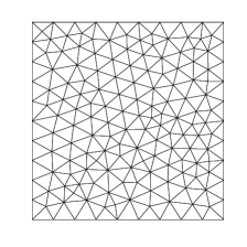
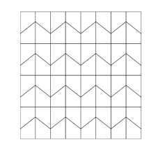
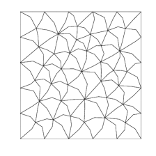
Figure 1. Sample meshes: $\mathcal{T}_{h}^{1}$ (left), $\mathcal{T}_{h}^{2}$ (middle) and $\mathcal{T}_{h}^{3}$ (right) with $h=0.1189$, $h=0.1719$ and $h=0.11078$, respectively.

We report in Table 1, Table 2 and Table 3 the relative errors in the discrete $L^{2}$-norm of $w$, $\nabla w$ and $\boldsymbol{\theta}$, together with the relative errors in the energy norm, for each family of meshes and different refinement levels. We consider different thickness: $t=1.0e-01$, $t=1.0e-02$ and $t=1.0e-03$, respectively. We also include in these table the experimental rate of convergence.

Table 1. $\mathcal{T}_{h}^{1}$: Computed error in the discrete $L^{2}$-norm with $t=1.0e-01$, $t=1.0e-02$ and $t=1.0e-03$, respectively.

error	$h=0.119$	$h=0.0588$	$h=0.0314$	$h=0.0158$	$h=0.00827$	Order
$e_{w}$	1.108e-01	2.941e-02	7.423e-03	1.841e-03	4.679e-04	2.06
$e_{\nabla w}$	1.300e-01	4.168e-02	1.321e-02	4.230e-03	1.502e-03	1.69
$e_{\boldsymbol{\theta}}$	8.873e-02	2.229e-02	5.434e-03	1.331e-03	3.367e-04	2.10
$\boldsymbol{\mathcal{E}}$	2.994e-01	1.278e-01	5.395e-02	2.276e-02	1.070e-02	1.26
$e_{w}$	1.030e-01	2.633e-02	6.493e-03	1.596e-03	4.041e-04	2.09
$e_{\nabla w}$	8.953e-02	2.255e-02	5.477e-03	1.343e-03	3.397e-04	2.10
$e_{\boldsymbol{\theta}}$	8.925e-02	2.244e-02	5.445e-03	1.335e-03	3.375e-04	2.10
$\boldsymbol{\mathcal{E}}$	1.756e-01	8.550e-02	4.199e-02	2.020e-02	1.029e-02	1.07
$e_{w}$	1.030e-01	2.631e-02	6.488e-03	1.596e-03	4.043e-04	2.09
$e_{\nabla w}$	8.926e-02	2.245e-02	5.452e-03	1.339e-03	3.387e-04	2.10
$e_{\boldsymbol{\theta}}$	8.926e-02	2.245e-02	5.452e-03	1.338e-03	3.387e-04	2.10
$\boldsymbol{\mathcal{E}}$	1.733e-01	8.475e-02	4.168e-02	1.998e-02	1.014e-02	1.07

Table 2. $\mathcal{T}_{h}^{2}$: Computed error in the discrete $L^{2}$-norm with $t=1.0e-01$, $t=1.0e-02$ and $t=1.0e-03$, respectively.

error	$h=0.172$	$h=0.0859$	$h=0.0430$	$h=0.0215$	$h=0.0122$	Order
$e_{w}$	3.890e-01	1.110e-01	2.958e-02	7.612e-03	1.868e-03	1.91
$e_{\nabla w}$	4.147e-01	1.370e-01	4.381e-02	1.405e-02	4.653e-03	1.61
$e_{\boldsymbol{\theta}}$	3.647e-01	9.742e-02	2.480e-02	6.247e-03	1.535e-03	1.96
$\boldsymbol{\mathcal{E}}$	6.267e-01	3.104e-01	1.345e-01	5.812e-02	2.527e-02	1.16
$e_{w}$	3.796e-01	1.037e-01	2.651e-02	6.656e-03	1.608e-03	1.96
$e_{\nabla w}$	3.663e-01	9.831e-02	2.501e-02	6.278e-03	1.534e-03	1.96
$e_{\boldsymbol{\theta}}$	3.659e-01	9.802e-02	2.490e-02	6.245e-03	1.525e-03	1.96
$\boldsymbol{\mathcal{E}}$	4.199e-01	1.675e-01	7.480e-02	3.619e-02	1.825e-02	1.12
$e_{w}$	3.795e-01	1.036e-01	2.650e-02	6.662e-03	1.612e-03	1.95
$e_{\nabla w}$	3.659e-01	9.803e-02	2.491e-02	6.254e-03	1.528e-03	1.96
$e_{\boldsymbol{\theta}}$	3.659e-01	9.803e-02	2.491e-02	6.253e-03	1.528e-03	1.96
$\boldsymbol{\mathcal{E}}$	4.154e-01	1.6465e-01	7.360e-02	3.548e-02	1.772e-02	1.12

Table 3. $\mathcal{T}_{h}^{3}$: Computed error in the discrete $L^{2}$-norm with $t=1.0e-01$, $t=1.0e-02$ and $t=1.0e-03$, respectively.

error	$h=0.111$	$h=0.0594$	$h=0.0294$	$h=0.0157$	$h=0.00791$	Order
$e_{w}$	2.848e-01	8.769e-02	2.421e-02	6.267e-03	1.569e-03	2.06
$e_{\nabla w}$	3.162e-01	1.202e-01	4.091e-02	1.338e-02	4.447e-03	1.70
$e_{\boldsymbol{\theta}}$	2.566e-01	7.465e-02	1.914e-02	4.740e-03	1.161e-03	2.14
$\boldsymbol{\mathcal{E}}$	6.371e-01	3.653e-01	1.690e-01	7.647e-02	3.470e-02	1.17
$e_{w}$	2.660e-01	7.407e-02	1.9065e-02	4.761e-03	1.161e-03	2.15
$e_{\nabla w}$	2.568e-01	7.495e-02	1.912e-02	4.778e-03	1.167e-03	2.14
$e_{\boldsymbol{\theta}}$	2.562e-01	7.460e-02	1.898e-02	4.736e-03	1.155e-03	2.15
$\boldsymbol{\mathcal{E}}$	3.793e-01	1.975e-01	9.555e-02	4.832e-02	2.365e-02	1.10
$e_{w}$	2.664e-01	7.458e-02	1.902e-02	4.742e-03	1.161e-03	2.18
$e_{\nabla w}$	2.561e-01	7.468e-02	1.907e-02	4.726e-03	1.161e-03	2.17
$e_{\boldsymbol{\theta}}$	2.560e-01	7.468e-02	1.907e-02	4.726e-03	1.161e-03	2.17
$\boldsymbol{\mathcal{E}}$	3.744e-01	1.904e-01	9.447e-02	4.757e-02	2.343e-02	1.11

It can be seen from Tables 1, 2 and 3 that the theoretical predictions of Section 4 are confirmed. In particular, we can appreciate a rate of convergence $O(h)$ for the energy norm $\boldsymbol{\mathcal{E}}$, that is equivalent to the $|||\cdot|||$ norm. This holds for all the considered meshes and thicknesses, thus also underlying the locking free nature of the scheme. Moreover, for sufficiently small $t$ we also observe a clear rate of convergence $O(h^{2})$ for for $e_{w}$, $e_{\nabla w}$ and $e_{\boldsymbol{\theta}}$, in accordance with Corollary 4.1.

5.2. Test 2:

As a second test, we investigate more in depth the locking-free character of the method, and also take the occasion for a comparison with the limit Kirchhoff model. It is well known (see [21]) that when $t$ goes to zero the solution of the Reissner-Mindlin model converges to an identical Kirchhoff-Love solution: Find $w_{0}\in{H^{2}(\Omega)}$ such that

(40) $$\dfrac{\mathbb{E}}{12(1-\nu^{2})}\Delta^{2}w_{0}=g,$$

with the corresponding boundary conditions.

We have considered a rectangular plate $\Omega:=(0,a)\times(0,b)$, simply supported on the whole boundary, and we have chosen the transversal load $g$ as

$$g(x,y)=\sin\left(\dfrac{\pi}{a}x\right)\sin\left(\dfrac{\pi}{b}y\right).$$

Then, the analytical solution $w_{0}$ of problem (40) is given by

$$w_{0}(x,y) =\dfrac{12(1-\nu^{2})}{\mathbb{E}}\left(\pi^{4}\left(\dfrac{1}{a^{2}}+\dfrac{1}{b^{2}}\right)^{2}\right)^{-1}\sin\left(\dfrac{\pi}{a}x\right)\sin\left(\dfrac{\pi}{b}y\right).$$

The material constants have been chosen $\mathbb{E}=1$ and $\nu=0.3$. Moreover, we have taken $a=1$ and $b=2$, and we have used three different families of meshes (see Figure 2):

• $\mathcal{T}_{h}^{1}$: triangular meshes;

• $\mathcal{T}_{h}^{4}$: hexagonal meshes;

• $\mathcal{T}_{h}^{5}$: Voronoi polygonal meshes.

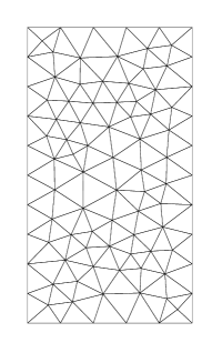
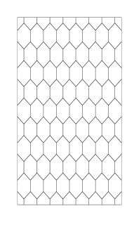
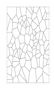
Figure 2. Sample meshes: $\mathcal{T}_{h}^{1}$ (left), $\mathcal{T}_{h}^{4}$ (middle) and $\mathcal{T}_{h}^{5}$ (right).

Tables 4, 5 and 6 show an analysis for various thicknesses in order to assess the locking-free nature of the proposed method. It is shown the relative errors in the discrete $L^{2}$-norm which are obtained by comparing the numerical solution with the Kirchhoff-Love plate solution $w_{0}$ for each family of meshes and different refinement levels and considering different thickness: $t=1.0e-01$, $t=1.0e-02$, $t=1.0e-03$, $t=1.0e-04$ and $t=1.0e-05$, respectively.

It can be clearly seen from these tables that the proposed method is locking-free. The lack of error reduction for finer values of $h$, which can be observed for the case $t=1.0e-01$, is clearly due to the fact that the model error is dominating the discretization error in those cases.

Table 4. Computed error in $e_{w}$ by $\mathcal{T}_{h}^{1}$.

$t\backslash h$	2.449e-01	1.271e-01	6.469e-02	3.241e-02	1.617e-02
1.0e-01	8.609e-03	4.090e-02	6.039e-02	7.108e-02	7.562e-02
1.0e-02	4.687e-02	1.034e-02	1.798e-03	7.665e-04	2.012e-03
1.0e-03	4.730e-02	1.096e-02	2.719e-03	6.668e-04	1.385e-04
1.0e-04	4.730e-02	1.097e-02	2.728e-03	6.823e-04	1.664e-04
1.0e-05	4.730e-02	1.097e-02	2.728e-03	6.825e-04	1.666e-04

Table 5. Computed error in $e_{w}$ by $\mathcal{T}_{h}^{4}$.

$t\backslash h$	2.781e-01	1.309e-01	6.730e-02	4.443e-02	3.316e-02
1.0e-01	8.394e-02	5.936e-02	6.256e-02	6.715e-02	6.910e-02
1.0e-02	4.979e-02	1.018e-02	4.022e-03	2.476e-03	2.095e-03
1.0e-03	4.943e-02	9.575e-03	3.145e-03	1.333e-03	7.381e-04
1.0e-04	4.942e-02	9.569e-03	3.136e-03	1.321e-03	7.228e-04
1.0e-05	4.942e-02	9.569e-03	3.136e-03	1.321e-03	7.227e-04

Table 6. Computed error in $e_{w}$ by $\mathcal{T}_{h}^{5}$.

$t\backslash h$	4.592e-01	2.348e-01	1.294e-01	8.174e-02	5.507e-02
1.0e-01	2.762e-02	4.055e-02	4.618e-02	6.510e-02	6.982e-02
1.0e-02	1.270e-02	3.454e-03	7.218e-04	1.141e-03	1.393e-03
1.0e-03	1.277e-02	3.004e-03	3.816e-04	6.483e-05	4.532e-05
1.0e-04	1.277e-02	2.999e-03	3.876e-04	6.248e-05	3.257e-05
1.0e-05	1.277e-02	2.999e-03	3.874e-04	6.215e-05	3.193e-05

5.3. Test 3:

In this numerical example we test the properties of the proposed method on an L-shaped plate: $\Omega:=(0,1)\times(0,1)\setminus[0.5,1)\times[0.5,1)$.

The plate is clamped on the edges $\{0\}\times[0,1]$, $\{1\}\times[0,1/2]$, $[0,1]\times\{0\}$, $[0,1/2]\times\{1\}$, and free on the remaining boundary and subjected to the constant transversal load $g=1$ (constant on the whole domain) and we take the material constants as $\mathbb{E}=1$ and $\nu=0$, with shear correction factor $k=5/6$. The thickness is set as $t=1.0e-01$.

We consider two families of meshes (see Figure 3):

• $\mathcal{T}_{h}^{6}$: a sequence of uniform squares meshes; the first one is constructed by subdividing into $8\times 8$ squares each of the three squares composing $\Omega$ (see upper left picture in Figure  3), up to the last one that is associated to an analogous $40\times 40$ subdivision.

• $\mathcal{T}_{h}^{7}$: polygonal meshes obtained following a very simple procedure that refines the mesh only around the re-entrant corner, starting from an initial uniform square mesh (that corresponds to the coarser mesh in $\mathcal{T}_{h}^{6}$). It consists of splitting each element which has the free corner $(1/2,1/2)$ as a vertex into four quadrilaterals by connecting the barycenter of the element with the midpoint of each edge. Notice that although this process is initiated with a mesh of squares, the successively created meshes will contain other kind of convex polygons as can be seen in Figure 3.

The main purpose of this test is to validate the use of refined meshes as a tool to handle solutions with corner singularities (therefore, in particular, not in $H^{3}(\Omega)$) and therefore overcome the theoretical limitation underlined in Remark 4.4. Moreover, the possibility of using polygonal meshes makes such refinement construction simpler, as shown by the example above; boundary layer treatment would obviously follow an analogous approach.

In Table 7 we report the value of the transversal displacement of the plate at the free corner $(1/2,1/2)$ and the number of degrees of freedom associated to each mesh. Since we have no exact solution for this problem, the last line in the table shows the reference values obtained with a very fine triangular mesh with the finite element method introduced and analyzed in [32]. We note that the family of meshes $\mathcal{T}_{h}^{7}$, being refined only around the corner, cannot obtain convergence as the error generated far from the corner would eventually dominate. Nevertheless, family $\mathcal{T}_{h}^{7}$ fits completely into the scope of the present test: comparing the displacement values obtained by $\mathcal{T}_{h}^{7}$ with those of the uniform meshes one can clearly appreciate the efficiency of the proposed corner refinement in handling the singularity.

Table 7. Test with an L-shaped plate. Number of degrees of freedom, transversal displacement of the free corner $(1/2,1/2)$ for the considered meshes, errors and a reference value for thickness $t=1.0e-01$.

	1541	0.01953427	2.0629e-04
	2345	0.01953098	2.0958e-04
	5765	0.01957589	1.6468e-04
	8885	0.01960441	1.3615e-04
$\mathcal{T}_{h}^{6}$	19625	0.01965190	8.8663e-05
	22277	0.01965845	8.2120e-05
	34565	0.01967856	6.2009e-05
ref.	181603	0.01974057
	1541	0.01953427	2.0629e-04
	1628	0.01965125	8.9314e-05
$\mathcal{T}_{h}^{7}$	1715	0.01970046	4.0110e-05
	1802	0.01972179	1.8778e-05
	1889	0.01973084	9.7313e-06
ref.	181603	0.01974057

Initial mesh (both for $\mathcal{T}_{h}^{6}$ and $\mathcal{T}_{h}^{7}$).

Mesh 2 of $\mathcal{T}_{h}^{7}$.

Mesh 3 of $\mathcal{T}_{h}^{7}$.

Mesh 6 of $\mathcal{T}_{h}^{7}$.

Figure 3. Sample meshes on L-shaped domain.

References

- [1] B. Ahmad, A. Alsaedi, F. Brezzi, L.D. Marini and A. Russo, Equivalent projectors for virtual element methods, Comput. Math. Appl., 66, (2013), pp. 376–391.
- [2] P.F. Antonietti, L. Beirão da Veiga, D. Mora and M. Verani, A stream virtual element formulation of the Stokes problem on polygonal meshes, SIAM J. Numer. Anal., 52(1), (2014), pp. 386–404.
- [3] P.F. Antonietti, L. Beirão da Veiga, S. Scacchi and M. Verani, A virtual element method for the Cahn–Hilliard equation with polygonal meshes, SIAM J. Numer. Anal., 54(1), (2016), pp. 36–56.
- [4] P.F. Antonietti, P. Houston, X. Hu, M. Sarti and M. Verani, Multigrid algorithms for -version interior penalty discontinuous Galerkin methods on polygonal and polyhedral meshes, Calcolo, DOI: 10.1007/s10092-017-0223-6 (2017).
- [5] D.N. Arnold, F. Brezzi, R.S. Falk and L.D. Marini, Locking-free Reissner-Mindlin elements without reduced integration, Comput. Methods Appl. Mech. Engrg., 196, (2007) pp. 3660–3671.
- [6] D.N. Arnold and R.S. Falk, A uniformly accurate finite element method for the Reissner-Mindlin plate, SIAM J. Numer. Anal., 26, (1989), pp. 1276–1290.
- [7] B. Ayuso de Dios, K. Lipnikov and G. Manzini, The nonconforming virtual element method, ESAIM Math. Model. Numer. Anal., 50(3), (2016), pp. 879–904.
- [8] L. Beirão da Veiga, F. Brezzi, A. Cangiani, G. Manzini, L.D. Marini and A. Russo, Basic principles of virtual element methods, Math. Models Methods Appl. Sci., 23, (2013), pp. 199–214.
- [9] L. Beirão da Veiga, F. Brezzi, L.D. Marini and A. Russo, The hitchhiker’s guide to the virtual element method, Math. Models Methods Appl. Sci., 24, (2014), pp. 1541–1573.
- [10] L. Beirão da Veiga, T.J.R. Hughes, J. Kiendl, C. Lovadina, J. Niiranen, A. Reali and H. Speleers, A locking-free model for Reissner-Mindlin plates: analysis and isogeometric implementation via NURBS and triangular NURPS, Math. Models Methods Appl. Sci., 25(8), (2015), pp. 1519–1551.
- [11] L. Beirão da Veiga, K. Lipnikov and G. Manzini, The Mimetic Finite Difference Method for Elliptic Problems, Springer, MS&A, vol. 11, 2014.
- [12] L. Beirão da Veiga, C. Lovadina and D. Mora, A virtual element method for elastic and inelastic problems on polytope meshes, Comput. Methods Appl. Mech. Engrg., 295, (2015) pp. 327–346.
- [13] L. Beirão da Veiga, C. Lovadina and A. Russo, Stability analysis for the virtual element method, Math. Models Methods Appl. Sci., DOI: 10.1142/S021820251750052X (2017).
- [14] L. Beirão da Veiga, C. Lovadina and G. Vacca, Divergence free virtual elements for the Stokes problem on polygonal meshes, ESAIM Math. Model. Numer. Anal., 51(2), (2017) pp. 509–535.
- [15] L. Beirão da Veiga, D. Mora, G. Rivera and R. Rodríguez, A virtual element method for the acoustic vibration problem, Numer. Math., 136(3), (2017) pp. 725–763.
- [16] M.F. Benedetto, S. Berrone, A. Borio, S. Pieraccini and S. Scialò, A hybrid mortar virtual element method for discrete fracture network simulations, J. Comput. Phys., 306, (2016), pp. 148–166.
- [17] M.F. Benedetto, S. Berrone, S. Pieraccini and S. Scialò, The virtual element method for discrete fracture network simulations, Comput. Methods Appl. Mech. Engrg., 280, (2014), pp. 135–156.
- [18] S. Bertoluzza, Substructuring preconditioners for the three fields domain decomposition method, Math. Comp. 73, (2004), pp. 659–689.
- [19] S.C. Brenner and R. L. Scott, The Mathematical Theory of Finite Element Methods, Springer, New York, 2008.
- [20] F. Brezzi, R.S. Falk and L.D. Marini, Basic principles of mixed virtual element methods, ESAIM Math. Model. Numer. Anal., 48, (2014), pp. 1227–1240.
- [21] F. Brezzi and M. Fortin, Mixed and Hybrid Finite Element Methods, Springer-Verlag, New York, (1991).
- [22] F. Brezzi, M. Fortin and R. Stenberg, Error analysis of mixed-interpolated elements for Reissner-Mindlin plates, Math. Models Meth. Appl. Sci., 1, (1991) pp. 125–151.
- [23] F. Brezzi and L.D. Marini, Virtual elements for plate bending problems, Comput. Methods Appl. Mech. Engrg., 253, (2012), pp. 455–462.
- [24] J. Bergh and J. Löfström, Interpolation spaces. An introduction. Springer-Verlag, Berlin–New York, 1976.
- [25] E. Caceres and G.N. Gatica, A mixed virtual element method for the pseudostress-velocity formulation of the Stokes problem, IMA J. Numer. Anal., 37(1), (2017) pp. 296–331.
- [26] A. Cangiani, E.H. Georgoulis and P. Houston, -version discontinuous Galerkin methods on polygonal and polyhedral meshes, Math. Models Methods Appl. Sci., 24(10), (2014), pp. 2009–2041.
- [27] C. Chinosi and C. Lovadina, Numerical analysis of some mixed finite element methods for Reissner-Mindlin plates, Comput. Mech., 16(1), (1995), pp. 36–44.
- [28] C. Chinosi and L.D. Marini, Virtual element method for fourth order problems: -estimates, Comput. Math. Appl., 72(8), (2016), pp. 1959–1967.
- [29] P.G. Ciarlet, The Finite Element Method for Elliptic Problems, SIAM, 2002.
- [30] P.G. Ciarlet, Interpolation error estimates for the reduced Hsieh–Clough–Tocher triangle, Math. Comp., 32(142), (1978), pp. 335–344.
- [31] D. Di Pietro and A. Ern, A hybrid high-order locking-free method for linear elasticity on general meshes, Comput. Methods Appl. Mech. Eng., 283, (2015), pp. 1–21.
- [32] R. Durán and E. Liberman, On mixed finite elements methods for the Reissner-Mindlin plate model, Math. Comput., 58, (1992), pp. 561–573.
- [33] R. Echter, B. Oesterle and M. Bischoff, A hierarchic family of isogeometric shell finite elements, Comput. Methods Appl. Mech. Engrg., 254, (2013) pp. 170–180.
- [34] R. Falk, Finite elements for the Reissner-Mindlin plate, D. Boffi and L. Gastaldi, editors, Mixed finite elements, compatibility conditions, and applications, Springer, Berlin, 2008, pp. 195–232.
- [35] A.L. Gain, C. Talischi and G.H. Paulino, On the virtual element method for three-dimensional linear elasticity problems on arbitrary polyhedral meshes, Comput. Methods Appl. Mech. Engrg., 282, (2014), pp. 132–160.
- [36] Q. Long, P.B. Bornemann and F. Cirak, Shear-flexible subdivision shells, Internat. J. Numer. Methods Engrg., 90(13), (2012) pp. 1549–1577.
- [37] C. Lovadina, A brief overview of plate finite element methods, Integral methods in science and engineering. Vol. 2, 261–280, Birkhäuser Boston, Inc., Boston, MA, 2010.
- [38] M. Lyly, J. Niiranen and R. Stenberg, A refined error analysis of MITC plate elements, Math. Models Methods Appl. Sci., 16, (2006), pp 967–977.
- [39] D. Mora, G. Rivera and R. Rodríguez, A virtual element method for the Steklov eigenvalue problem, Math. Models Methods Appl. Sci., 25(8), (2015), pp. 1421–1445.
- [40] G.H. Paulino and A.L. Gain, Bridging art and engineering using Escher-based virtual elements, Struct. Multidiscip. Optim., 51(4), (2015), pp. 867–883.
- [41] I. Perugia, P. Pietra and A. Russo, A plane wave virtual element method for the Helmholtz problem, ESAIM Math. Model. Numer. Anal., 50(3), (2016), pp. 783–808.
- [42] S. Rjasanow and S. Weißer, Higher order BEM-based FEM on polygonal meshes, SIAM J. Numer. Anal., 50(5), (2012), pp. 2357–2378.
- [43] L.R. Scott and S. Zhang, Finite element interpolation of nonsmooth functions satisfying boundary conditions, Math. Comp. 54, (1990), pp. 483–493.
- [44] E. M. Stein, Singular integrals and differentiability properties of functions, volume 2. Princeton University Press, 1970.
- [45] N. Sukumar and A. Tabarraei, Conforming polygonal finite elements, Internat. J. Numer. Methods Engrg., 61, (2004), pp. 2045–2066.
- [46] C. Talischi, G.H. Paulino, A. Pereira and I.F.M. Menezes, Polygonal finite elements for topology optimization: A unifying paradigm, Internat. J. Numer. Methods Engrg., 82(6), (2010), pp. 671–698.
- [47] P. Wriggers, W.T. Rust and B.D. Reddy, A virtual element method for contact, Comput. Mech., 58, (2016), pp. 1039–1050.
- [48] J. Zhao, S. Chen and B. Zhang, The nonconforming virtual element method for plate bending problems, Math. Models Methods Appl. Sci., 26(9), (2016), pp. 1671–1687.