Collective modes in multicomponent condensates with anisotropy

Abstract

We report the effects of anisotropy in the confining potential on two component Bose-Einstein condensates (TBECs) through the properties of the low energy quasiparticle excitations. Starting from generalized Gross Pitaevskii equation, we obtain the Bogoliubov de-Gennes (BdG) equation for TBECs using the Hartree-Fock-Bogoliubov (HFB) theory. Based on this theory, we present the influence of radial anisotropy on TBECs in the immiscible or the phase-separated domain. In particular, the TBECs of ⁸⁵Rb -⁸⁷Rb and ¹³³Cs -⁸⁷Rb TBECs are chosen as specific examples of the two possible interface geometries, shell-structured and side by side, in the immiscible domain. We also show that the dispersion relation for the TBEC shell-structured interface has two branches, and anisotropy modifies the energy scale and structure of the two branches.

I Introduction

The physics of trapped ultra-cold atoms, specifically the Bose Einstein condensate (BEC), is replete with novel phenomena emerging from the atom-atom interactions, trap geometry, quantum and thermal fluctuations, topological defects, spatial dimensions and so on. In particular, the geometry of the confining potential has a strong impact on the density profiles of the single component as well as on the multi-component BECs. An example is, in a three dimensional (3D) harmonic potential, if the axial frequency ($\omega_{z}$) is much larger than the radial frequencies ($\omega_{x}=\omega_{y}=\omega_{\perp}$), the condensate is effectively 2D with pancake shaped density profile. The symmetric radial frequencies is an ideal situation, and in experiments, there are deviations from symmetry due to practical limitations of the various components. For example, the pioneering experiments on BECs Davis et al. (1995); Anderson et al. (1995) were done in anisotropic trap. Thus, it is of practical importance to consider anisotropic radial confinement ($\omega_{x}\neq\omega_{y}$) and examine the deviations from the symmetric case. With this consideration, in the present work, we study the effects of radial anisotropy arising from the confining potential at zero temperature. An immediate consequence of the anisotropy is the change of interface geometry of the multicomponent condensates at phase-separation.

The inter-atomic interactions play dramatic role in low dimensional, quasi 1D and 2D, BECs of trapped atomic gases. With quasi low dimensional BECs, there are excitations unique to each which do not have an analogue in the higher or lower dimensional BECs. In our previous works, we characterized the low energy excitation modes for quasi 1D Roy et al. (2015) and quasi 2D Roy and Angom (2016) BEC. Apart from this, in the TBECs the miscible-immiscible phase transition has strong dimensional dependence. At zero temperature, the condition of phase separation under Thomas-Fermi (TF) approximation is given by the inequality $U^{2}_{12}>U_{11}U_{22}$ Timmermans (1998); Pu and Bigelow (1998); Ho and Shenoy (1996).

In this work, we report the transition from circular to planar interface with increased anisotropy Gautam and Angom (2010); Mertes et al. (2007) in the TBECs with shell structured density configuration in the immiscible domain. We also demonstrate that the transformation in the interface geometry leads to a change in the low energy excitation modes. As a representative example of the shell structured interface we choose ⁸⁵Rb -⁸⁷Rb TBEC which is experimentally well studied Papp and Wieman (2006); Papp et al. (2008). The other density configuration of a TBEC in the immiscible domain is the side by side density profiles. For this case as well, we show that the presence of anisotropy leads to distinct structures of the density profiles in the immiscible domain. This is accompanied by the changes in the low energy BdG spectrum and structure of the quasiparticle amplitudes. We consider the ¹³³Cs -⁸⁷Rb TBEC McCarron et al. (2011) as a representative example for this case.

The dispersion relation is the key to understand how the TBEC responds to external perturbations. So, to relate theoretical investigations with experimental findings, it is essential to determine how the dispersion relation of TBECs change with anisotropy. In this context analysing the observations from the Bragg Bogoliubov spectrum which in turn necessitates knowledge of dispersion relations. Theoretically, dispersion relation for BEC has been investigated in the analytic framework Pethick and Smith (2008). In addition, there are several numerical computations of the dispersion relations in finite sized BEC Wilson et al. (2010); Bisset and Blakie (2013); Blakie et al. (2012) in presence of roton like spectrum. The dispersion relations and characterization of excitation modes both in single component BEC Ticknor et al. (2011) and TBEC Ticknor (2014) have been investigated in the miscible and immiscible (side by side configuration) phases. In the present study, we study dispersion relations in the immiscible phase for both the side by side and shell structured density configurations. More important, the effect of radial anisotropy on dispersion relations are investigated for both the configurations. A recent work Klaiman et al. (2017) has also reported the pathway from condensation towards fragmentation arising from the anisotropy of the confining potential. We also observe anisotropy enhanced fragmentation of the outer species in a shell structured immiscible TBEC.

The purpose of this paper is to present a systematic study to capture the influences of radial anisotropy in segregated condensate mixtures. This paper is organized as follows. In Sec. II we provide a brief description of the HFB-Popov formalism for quasi-2D BEC. We then give the discrete dispersion relation used in the numerical computations. The results and discussions are presented in Sec. III for two representative TBECs, namely ⁸⁵Rb -⁸⁷Rb and ¹³³Cs -⁸⁷Rb TBECs. Sec. III.1 presents the discussions on the effects of radial anisotropy on density profiles and mode evolution of ⁸⁵Rb -⁸⁷Rb TBEC in immiscible regime. This is followed with computation of dispersion relation and the consequences of radial anisotropy on it presented in Sec. III.2. In the next two sections, Sec. III.3 and Sec. III.4, we discuss the density profile, mode evolution and dispersion relation of the ¹³³Cs -⁸⁷Rb TBEC. We, then, end the main part of the paper with conclusions in Sec. IV.

II Theory

Mean field calculations based on Popov approximation to Hartree-Fock Bogoliubov theory (HFB) has been of paramount importance in determining the finite temperature effects and frequencies of collective excitations. To start with, we briefly describe the HFB theory for a quasi-2D (pancake shaped) TBEC trapped in an anisotropic harmonic potential. This implies that the frequencies of the harmonic potential satisfies the conditions $\omega_{x},\omega_{y}\ll\omega_{z}$ and $\omega_{x}\neq\omega_{y}$. So, the confining potential is of the form

$$V_{k}(x,y,z)=(1/2)m_{k}\omega_{x}^{2}(x^{2}+\alpha^{2}y^{2}+\lambda^{2}z^{2}),$$ (1)

where, $\alpha=\omega_{y}/\omega_{x}$, and $\lambda=\omega_{z}/\omega_{x}$ are the anisotropy parameters. In terms of these parameters the requirement to have a quasi-2D geometry is $\lambda\gg 1$, $\hbar\omega_{z}\gg\mu_{k}$. This strongly confines the motion of the trapped atoms along the $z$-axis and in this direction the atoms are frozen in the ground state Petrov et al. (2000). However, excitations are allowed along the $xy$-plane and making the system kinematically 2D. Under the mean field approximation, a quasi-2D TBEC of interacting bosons is described by the grand-canonical Hamiltonian

$$\hat{H} = \sum_{\begin{subarray}{c}k=1,2\end{subarray}}\iint dxdy\hat{\Psi}_{k}^{\dagger}(x,y,t)\Bigg{[}-\frac{\hbar^{2}}{2m_{k}}\nabla^{2}_{\perp}+V_{k}(x,y)-\mu_{k}$$ (2)

$$+\frac{U_{kk}}{2}\hat{\Psi}_{k}^{\dagger}(x,y,t)\hat{\Psi}_{k}(x,y,t)\Bigg{]}\hat{\Psi}(x,y,t)+~{}~{}U_{12}\iint dxdy$$

$$\times\hat{\Psi}_{1}^{\dagger}(x,y,t)\hat{\Psi}_{2}^{\dagger}(x,y,t)\hat{\Psi}_{1}(x,y,t)\hat{\Psi}_{2}(x,y,t),$$

with $k=1,2$ denoting the species index, $\hat{\Psi}_{k}$ ($\hat{\Psi}_{k}^{\dagger}$) are the Bose field annihilation (creation) operators of the two species, and $\mu_{k}$s are the chemical potentials. In quasi-2D, $U_{kk}=2a_{kk}\sqrt{2\pi\lambda}$ and $U_{12}=2a_{12}\sqrt{2\pi\lambda}(1+m_{1}/m_{2})$ are the intra-species and inter-species interactions, respectively. Here, $a_{kk}$, $a_{12}$ are the $s$-wave intra- and interspecies scattering lengths. In the present work we consider only repulsive interactions and hence, $a_{kk}>0$, $a_{12}>0$. From the Hamiltonian in Eq. (2), the dynamics of Bose field operators are given by the coupled equations

$$\begin{aligned} i\hbar\begin{pmatrix}\dot{\hat{\Psi}}_{1}\\ \dot{\hat{\Psi}}_{2}\end{pmatrix}\!\!=\!\!\begin{pmatrix}\hat{h}_{1}+U_{11}\hat{\Psi}_{1}^{\dagger}\hat{\Psi}_{1}&U_{12}\hat{\Psi}_{2}^{\dagger}\hat{\Psi}_{1}\\ U_{12}\hat{\Psi}_{1}^{\dagger}\hat{\Psi}_{2}&\hat{h}_{2}+U_{22}\hat{\Psi}_{2}^{\dagger}\hat{\Psi}_{2}\end{pmatrix}\!\!\!\begin{pmatrix}\hat{\Psi}_{1}\\ \hat{\Psi}_{2}\end{pmatrix},\end{aligned}$$ (3)

where, $\hat{h}_{k}=(-\hbar^{2}/2m_{k})\nabla_{\perp}^{2}+V_{k}(x,y)-\mu_{k}$ is the single-particle part of the Hamiltonian.

When the temperature is below the critical temperature ($T_{c}$), majority of the atoms occupy the ground state to form a condensate. Thus for $T\ll T_{c}$ following the Bogoliubov decomposition, the Bose field operator can be expressed as the sum of condensate part and the fluctuations over it $\hat{\Psi}_{k}=\phi_{k}+\tilde{\psi}_{k}$, where $\phi_{k}=\langle\hat{\Psi}_{k}\rangle$s are the $c$-fields representing each of the condensate species, and $\tilde{\psi}_{k}$s are the corresponding non-condensate densities or fluctuations which may be either quantum or thermal in nature. By definition the fluctuation operators satisfy the condition $\langle\tilde{\psi}_{k}\rangle=\langle\tilde{\psi}_{k}^{\dagger}\rangle=0$. In addition, on the application of time-independent HFB-Popov approximation Griffin (1996), Eq. (3) reduces to the coupled generalized Gross-Pitaevskii (CGGP) equations

$$\hat{h}_{k}\phi_{k}+U_{kk}\left[n_{ck}+2\tilde{n}_{k}\right]\phi_{k}+U_{12}n_{3-k}\phi_{k}=0,$$ (4)

where, $\phi_{k}$s is the stationary solutions of CGGP with $n_{ck}(x,y)\equiv|\phi_{k}(x,y)|^{2}$, $\tilde{n}_{k}(x,y)\equiv\langle\tilde{\psi}^{\dagger}(x,y,t)\tilde{\psi}(x,y,t)\rangle$ and $n_{k}(x,y)=n_{ck}(x,y)+\tilde{n}_{k}(x,y)$ represent the local condensate, non-condensate and total density respectively. Employing Bogoliubov transformation, fluctuations $\tilde{\psi}_{k}$ and its complex conjugate $\tilde{\psi}_{k}^{\dagger}$ are expressed as the linear combination of quasiparticle creation ($\hat{\alpha}_{j}^{\dagger}$) and annihilation ($\hat{\alpha}_{j}$) operators Ticknor (2014)

$$\begin{aligned} \tilde{\psi}_{k}&=&\sum_{j}\big{[}u_{kj}(x,y)\hat{\alpha}_{j}e^{-i\varepsilon_{j}t/\hbar}-v_{kj}^{\ast}(x,y)\hat{\alpha}_{j}^{\dagger}e^{i\varepsilon_{j}^{\ast}t/\hbar}\big{]},\\ \tilde{\psi}_{k}^{\dagger}&=&\sum_{j}\big{[}u_{kj}^{\ast}(x,y)\hat{\alpha}_{j}^{\dagger}e^{i\varepsilon_{j}^{\ast}t/\hbar}-v_{kj}(x,y)\hat{\alpha}_{j}e^{-i\varepsilon_{j}t/\hbar}\big{]},\end{aligned}$$ (5)

where $j$ is the index representing the sequence of the quasiparticle excitation. The quasiparticle creation and annihilation operators satisfy the usual Bose commutation relations. $u_{jk}$ and $v_{jk}$ are complex functions and denote the Bogoliubov quasiparticle amplitudes with the normalisation

$$\iint dxdy\sum_{k}\left(|u_{k}(x,y)|^{2}-|v_{k}(x,y)|^{2}\right)=1.$$ (6)

Considering all the above decompositions and transformations, the equation of motion of the fluctuation operator are

$$\hat{{\mathcal{L}}}_{1}u_{1j}-U_{11}\phi_{1}^{2}v_{1j}+U_{12}\phi_{1}\left(\phi_{2}^{*}u_{2j}-\phi_{2}v_{2j}\right) = \varepsilon_{j}u_{1j},\;\;\;\;\;\;$$ (7a)

$$\hat{\underline{\mathcal{L}}}_{1}v_{1j}+U_{11}\phi_{1}^{*2}u_{1j}-U_{12}\phi_{1}^{*}\left(\phi_{2}v_{2j}-\phi_{2}^{*}u_{2j}\right) = \varepsilon_{j}v_{1j},\;\;\;\;\;\;$$ (7b)

$$\hat{{\mathcal{L}}}_{2}u_{2j}-U_{22}\phi_{2}^{2}v_{2j}+U_{12}\phi_{2}\left(\phi_{1}^{*}u_{1j}-\phi_{1}v_{1j}\right) = \varepsilon_{j}u_{2j},\;\;\;\;\;\;$$ (7c)

$$\hat{\underline{\mathcal{L}}}_{2}v_{2j}+U_{22}\phi_{2}^{*2}u_{2j}-U_{12}\phi_{2}^{*}\left(\phi_{1}v_{1j}-\phi_{1}^{*}u_{1j}\right) = \varepsilon_{j}v_{2j},\;\;\;\;\;\;\;\;\;$$ (7d)

which are referred as the Bogoliubov-de-Gennes equations for the quasi-2D TBEC system Ticknor (2013); Roy et al. (2014) with $\hat{{\mathcal{L}}}_{1}=\big{(}\hat{h}_{1}+2U_{11}n_{1}+U_{12}n_{2})$, $\hat{{\mathcal{L}}}_{2}=\big{(}\hat{h}_{2}+2U_{22}n_{2}+U_{12}n_{1}\big{)}$ and $\hat{\underline{\cal L}}_{k}=-\hat{\cal L}_{k}$.

To solve Eq. (7), $u_{kj}$s and $v_{kj}$s are written as a linear combination of the harmonic oscillator eigenstates and the Bogoliubov-de-Gennes matrix (BdGM) constructed from Eq. (7) is diagonalized. Eq. (7) along with Eq. (4) are known as Hartree-Fock Bogoliubov (HFB) equations and need to be solved self consistently. The solutions are the order parameters $\phi_{k}$s and the non-condensate densities $\tilde{n}_{k}$s. The thermal components, in terms of the quasiparticle amplitudes, are

$$\tilde{n}_{k}=\sum_{j}\left[(|u_{kj}|^{2}+|v_{kj}|^{2})N_{0}(\varepsilon_{j})+|v_{kj}|^{2}\right],$$ (8)

where, $N_{0}(\varepsilon_{j})=(e^{\beta\varepsilon_{j}}-1)^{-1}$ with $\beta=1/(k_{\rm B}T)$ is the Bose factor of the $j$th quasiparticle mode at temperature $T$. As $T$ approaches to zero, the role of thermal fluctuations gradually diminishes. At $T=0$, thermal fluctuations is absent and the non-condensate density arises only from the quantum fluctuations, which is evident from Eq. (8) as it is reduced to $\tilde{n}_{k}=\sum_{j}|v_{kj}|^{2}$ at $T=0$. Our studies show that the $\tilde{n}_{k}$ arising from the quantum fluctuations does not produce significant changes in the BdG spectrum, and so, we avoid the condition of self-consistency at zero temperature. The details of the numerical scheme adopted to compute the Bogoliubov quasiparticle amplitudes and fluctuations has been elaborated in Ref. Pal et al. (2017).

The dispersion relations determine the response of a physical system when subjected to external perturbations. For the present work, the change in the geometry of the interface in a TBEC arising from a change in the anisotropy of the confining potential affects the energies and amplitudes of the quasiparticle excitations. In the limit of low $\alpha$, the TBECs consist of three topologically connected fragments. The dispersion relation is thus expected to change. To define the dispersion relation we compute the root mean square of the wave number $k^{\rm rms}$ of each quasiparticle mode, and the results describes a discrete dispersion relation. Following Refs. Ticknor (2014); Wilson et al. (2010), the $k^{\rm rms}$ of the $j$th quasiparticle is

$$k_{j}^{\rm rms}=\left\{\frac{\sum_{i}\int d\mathbf{k}k^{2}[|u_{ij}(\mathbf{k})|^{2}+|v_{ij}(\mathbf{k})|^{2}]}{\sum_{i}\int d\mathbf{k}[|u_{ij}(\mathbf{k})|^{2}+|v_{ij}(\mathbf{k})|^{2}]}\right\}^{1/2}.$$ (9)

It is to be noted here that $k_{j}^{\rm rms}$ are defined in terms of the quasiparticle modes corresponding to each of the constituent species defined in the $k$ or momentum space through the index $i=1,2$. It is then essential to compute $u_{j}(\mathbf{k})$ and $v_{j}(\mathbf{k})$, the Fourier transform of the Bogoliubov quasiparticle amplitudes $u_{j}(x,y)$ and $v_{j}(x,y)$, respectively. Once we have $k_{j}^{\rm rms}$ for all the modes we obtain a dispersion curve, and we can then examine how the change in the condensate topology modifies the dispersion curve.

III Results and Discussions

In a trapped quasi-2D TBEC, the low-lying BdG spectrum supports two Goldstone modes for each of the condensate species due to breaking of $U(1)$ global gauge symmetry. The two lowest modes corresponding to each of the species with non zero excitation energies are called the dipole modes. The dipole modes which oscillate out-of-phase with each other are called slosh modes. In-phase slosh modes with center-of-mass motion are called the Kohn modes. The frequency of the Kohn mode is independent of the type of interactions and interaction strength as well. The presence of the Kohn modes in the trapped system follows from Kohn’s theorem Kohn (1961); Fetter and Rokhsar (1998). According to the theorem BEC in a confining potential must have a mode in which the centre of mass oscillates with the frequency of the confining potential. However, in a magnetic trap in the vicinity of the Feshbach resonance Al-Jibbouri and Pelster (2013) and in few-electron parabolic quantum dots doped with a single magnetic impurity Nguyen and Peeters (2010), there are deviations from Kohn’s theorem.

A variation in the interaction strength drives the TBEC system from immiscible to miscible configuration or vice versa. In addition, it can induce dynamical instability resulting in the swapping of the species. But, the radial anisotropy can alter the equilibrium density distribution of the ground state and modify the evolution of low lying mode energies. Among the low lying modes of the BdG spectrum, the dipole (Kohn/slosh) and quadrupole modes have dominant contribution to $\tilde{n}$ at $T\sim 0$K and hence we examine these modes detail. The transformation of these modes due to radial anisotropy is one of the primary issues addressed in this paper, and as example we consider specific systems.

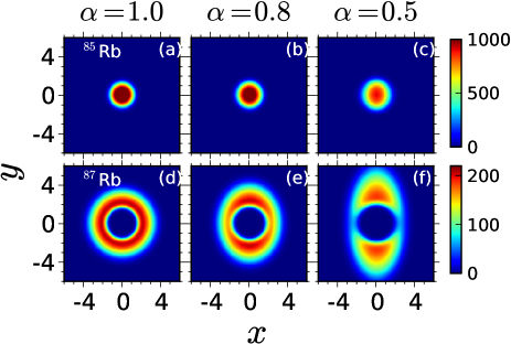
Figure 1: (Color online) Equilibrium condensate density profiles of ⁸⁵Rb -⁸⁷Rb TBEC at zero temperature for three different values of $\alpha$ ($\alpha$ = 1.0, 0.8, 0.5). $a_{11}$ is kept fixed at $10a_{0}$ . (a)-(c) Equilibrium density profiles corresponding to ⁸⁵Rb. (d)-(f)Equilibrium density profiles corresponding to ⁸⁷Rb. $n_{c}$ is measured in units of $a_{\rm osc}^{-2}$ and the spatial coordinates $x$ and $y$ are measured in units of $a_{\rm osc}$.

III.1 Mode evolution of ⁸⁵Rb -⁸⁷Rb BEC mixture

In this section, we consider the TBEC of homonuclear atoms at zero temperature with shell structured density profile in immiscible domain. We choose ⁸⁵Rb -⁸⁷Rb TBEC as a representative example. For convenience, we designate atoms of ⁸⁵Rb and ⁸⁷Rb as species 1 and 2, respectively. The intra-species scattering length of ⁸⁷Rb atoms has the value $a_{22}=99a_{0}$, and the inter-species scattering length $a_{12}=214a_{0}$. We consider equal number of atoms for the two species, i.e, $N_{1}=N_{2}=5000$ and the quasi-2D Rb-Rb TBEC that we considered here is obtained with trapping parameters $\lambda=12.5$ and $\omega_{x}=2\pi\times 8.0$Hz Neely et al. (2010). Here, it is to be emphasized that the background intra-species scattering length of ⁸⁵Rb ($a_{11}$) is negative, and to obtain BEC of ⁸⁵Rb it is essential to tune the scattering length to positive values using magnetic Feshbach resonance Cornish et al. (2000). For the present work we perform our calculations for three different values of $a_{11}=10a_{0},50a_{0},180a_{0}$. With this specific set of trapping and interaction parameters, at equilibrium, the ground state of the TBEC is phase-separated with shell structured density profile. For $\alpha=1$, (i.e., for $\omega_{x}=\omega_{y}$) the TBEC is rotationally symmetric and the interface separating the two condensates is circular. However, for $\alpha<1$ the rotational symmetry is broken with the density profile of the condensates elongated along $y$ direction and as $\alpha$ is decreased the interface transforms from circular to planar

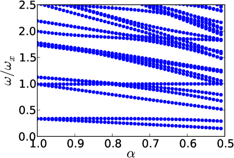
Figure 2: (Color online) The evolution of low-lying quasiparticle modes in the phase separated domain of ⁸⁵Rb -⁸⁷Rb TBEC as a function of $\alpha$ in the domain $0.5\leq\alpha\leq 1.0$ for $a_{11}=10a_{0}$ at zero temperature with $N_{1}=N_{2}=5000$.

In Fig. 1 we show the equilibrium condensate density profiles for $a_{11}$ = 10 $a_{0}$ for $\alpha=1.0,0.8$ and $0.5$. As the profiles show TBEC is phase-separated with ⁸⁵Rb atoms lying at the center surrounded by the ⁸⁷Rb atoms. With decreasing $\alpha$, the density profiles are modified and are fragmented at lower values of $\alpha$. In the figure, the fragmentation is discernible for $\alpha=0.5$, where the condensate density profile of ⁸⁷Rb appears to consist of two symmetric lobes equidistant from the origin. For all the three cases, ⁸⁵Rb condensate remains at the core and with lower values of $\alpha$ it expands along $y$-direction and changes its geometry from circular to ellipse with $y$-axis being the major axis. The change in the density distribution also affects the quasiparticle excitation spectrum. For $a_{11}=10a_{0}$, the quasi particle mode evolution as a function of $\alpha$ is shown in Fig. 2. As seen from the figure the degeneracies of the mode energies are lifted when $\alpha<1$. For the dipole mode, as the degeneracy is lifted the Kohn mode remains steady at $\omega=\omega_{x}$ whereas the energy of the slosh mode decreases.

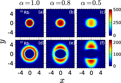
Figure 3: (Color online) Equilibrium condensate density profiles of ⁸⁵Rb -⁸⁷Rb TBEC at zero temperature for three different values of $\alpha$ ($\alpha$ = 1.0, 0.8, 0.5). $a_{11}$ remains fixed at $50a_{0}$ . (a)-(c) Equilibrium density profiles corresponding to ⁸⁵Rb (d)-(f)Equilibrium density profiles corresponding to ⁸⁷Rb. Equilibrium condensate density $n_{c}$ is measured in units of $a_{\rm osc}^{-2}$ and the spatial coordinates $x$ and $y$ are measured in units of $a_{\rm osc}$.

For the isotropic case ( $\alpha=1$) the ⁸⁵Rb -⁸⁷Rb TBEC is dynamically unstable in the region $50a_{0}\leqslant a_{11}\leqslant 150a_{0}$ Pal et al. (2017). The presence of anisotropy affects the dynamical instability of the mixture and with the increase of $\alpha$ instability decreases. Thus, both the onset of instability and the radial anisotropy can have a major influence on the equilibrium density profile at $a_{11}=50a_{0}$. As shown in Fig. 3, the density profiles do exhibit a transformation as a function of $\alpha$ at $a_{11}=50a_{0}$. The equilibrium density profile in Fig. 3(f) shows that unlike Fig. 1, the two lobes of ⁸⁷Rb are disconnected. In addition, when $a_{11}>a_{22}$, the species swaps their positions and the density profile of ⁸⁵Rb -⁸⁷Rb TBEC has similar configuration as was for $a_{11}<a_{22}$. For example, with $a_{11}=180a_{0}$ and $a_{22}=99a_{0}$, the equilibrium density profile of ⁸⁵Rb -⁸⁷Rb TBEC has the similar configuration as shown in Fig. 1 but with species positions interchanged. To examine the further, the low lying mode energies are shown as a function of $\alpha$ in Fig. 4. Unlike in the case of $a_{11}=10a_{0}$ there is a doubly degenerate zero energy mode. In addition, some of the low-lying modes show a decrease in energy up to $\alpha\approx 0.7$, and increase for $\alpha<0.7$. The important point to note is that the new zero energy mode remains degenerate upto $\alpha=0.65$. But, for $\alpha<0.65$ the degeneracy is lifted and the mode energy bifurcates into two branches. One branch continues to be the zero energy mode, where as the other branch becomes hard. Similarly, the doubly degenerate quadrupole mode with energy $\hbar\omega\approx 0.6\hbar\omega_{x}$ at $\alpha=1$ continue to soften and at $\alpha\approx 0.8$ the degeneracy is lifted creating two branches. For $\alpha<0.8$, both the branches continue to soften but at $\alpha\approx 0.7$ the branches start to harden. The hardening and softening of the low energy quasiparticle modes have also been observed around the point of phase separation of TBECs in optical lattices Suthar et al. (2015); Suthar and Angom (2016), and due to the change in the geometry and topology of the confining potential Roy and Angom (2016).

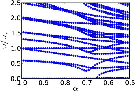
Figure 4: (Color online) The evolution of low-lying mode energies as a function of $\alpha$ in the phase separated domain of ⁸⁵Rb -⁸⁷Rb TBEC at zero temperature. $\alpha$ is varied in the domain $0.5\leqslant\alpha\leqslant 1.0$ while $a_{11}$ is kept fixed at $50a_{0}$. For ⁸⁵Rb -⁸⁷Rb TBEC, it is a domain of interest since dynamical instability sets in at $a_{11}=50a_{0}$ for $N_{1}=N_{2}=5000$.

III.2 Excitations and dispersion relations for ⁸⁵Rb -⁸⁷Rb TBEC

The dispersion curves are computed based on Eq. (9). This involves computing the $k^{\rm rms}$ of the $j$th quasiparticle, and then the corresponding quasiparticle mode energies are plotted as function of the $k^{\rm rms}$. In the miscible domain the dispersion curve is expected to be devoid of structures as the quasiparticle amplitudes of the component BECs are similar. However, in the immiscible domain the vastly different density distributions of the two species lead to diverse quasiparticle amplitude structures. And, this can manifest as structures in the dispersion curves. As a specific example, consider the case of shell structured immiscible density distribution of ⁸⁵Rb -⁸⁷Rb TBEC. In spite of rotational symmetry, due to immiscible domain the dispersion curves shown in Fig. 5 exhibit complex trends.

In Fig. 5(a) the dispersion relation at $\alpha=1.0$ for ⁸⁵Rb -⁸⁷Rb TBEC in immiscible (sandwich) domain with $a_{11}=10a_{0}$ is shown. The dispersion curve has two well separated branches: the upper branch starts at $\approx 6.35\hbar\omega_{x}$ and the lower branch starts close to zero energy. This is in contrast to the dispersion relations reported for the immiscible TBEC with side by side configuration. One important reason to study dispersion curves is to identify modes with different characteristics. In the present case the two well separated modes correspond to two different classes of excitations: the interface and bulk excitations. To analyze these two branches in better detail we plot selected quasiparticle amplitudes from these two branches. For the lower branch, the quasiparticle amplitudes of the modes marked with red empty circle $({\color[rgb]{1,0,0}\bigcirc})$ are shown in Fig. 6. These modes with low-$k$ have high energies and are localized at the interface of the two species.

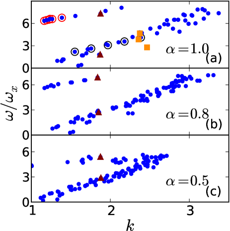
Figure 5: (Color online) (a) The dispersion relation for immiscible (shell structured) ⁸⁵Rb -⁸⁷Rb TBEC at $a_{11}$=10$a_{0}$ when $\alpha=1.0$. In this plot the dispersion curves can be broadly classified into two broadly separated branches. The quasi particle amplitudes corresponding to the upper branch marked with red empty circles $({\color[rgb]{1,0,0}\bigcirc})$ are shown in Fig. 6. For the lower branch the quasi particle amplitudes is shown in Fig. 7 along a particular path marked with empty black circle $({\color[rgb]{0,0,0}\bigcirc})$. (b) The dispersion relation for immiscible (shell structured) ⁸⁵Rb -⁸⁷Rb TBEC at $a_{11}$=10$a_{0}$ when $\alpha=0.8$. (c) The dispersion relation for immiscible (shell structured) ⁸⁵Rb -⁸⁷Rb TBEC at $a_{11}$=10$a_{0}$ when $\alpha=0.5$. As value of $\alpha$ is reduced from 1.0 i.e., radial anisotropy makes this two branches comparatively closer to each other.

In Fig. 6(a)(i-vi) the interface excitations for ⁸⁵Rb, the condensate species which occupies the central region, are shown. The interface nature of the quasiparticles is discernible from the geometry as these have non-zero values only at the interface. With the increase of energy, numerical values annotated at the top of each column, azimuthal quantum number ($m$) increases. It must be mentioned that in the figures, for information the energies are listed up to the fifth decimal, and this is not an indication of the accuracy. So, here after for the description of the results we list only up to the second decimal. To illustrate the change in $m$ consider Fig. 6(a)(ii), which corresponds to mode with energy $6.44\hbar\omega_{x}$ and corresponds to $m=1$. Whereas the mode in Fig. 6 (a)(vi) which has larger number of lobes and corresponds to $m=3$ has energy $6.77\hbar\omega_{x}$. On the other hand, Fig. 6(b)(i-vi) show the interface excitations for ⁸⁷Rb. Since it is energetically favorable for the outer species to expand, the quasiparticles corresponding to ⁸⁷Rb are composed of four radial nodes with $m$ being directly proportional to the mode energy.

For the lower branch the quasiparticle amplitudes of few specific modes marked with black empty circle $({\color[rgb]{0,0,0}\bigcirc})$ are shown in Fig. 7. These are the bulk excitations of the TBEC mixture. Like in the previous case, Fig. 7(a)(1-6) show the quasiparticle amplitudes for ⁸⁵Rb, and Fig. 7(b)(1-6) correspond to ⁸⁷Rb. The modes are marked with black empty circle $({\color[rgb]{0,0,0}\bigcirc})$ and these trace a path in the dispersion curve from small-$k$ towards large-$k$. Along the path the quasiparticles have one radial node and it is discernible in the quasiparticle amplitudes of both the species. The azimuthal quantum number $m$ increases with the increase of mode energy. The bulk nature of the excitations is manifest from the structure of the quasiparticle amplitudes as they coincide with the condensate density distribution.

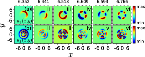
Figure 6: (Color online) Quasiparticle amplitudes corresponding to interface excitations for the immiscible (shell structured) ⁸⁵Rb -⁸⁷Rb TBEC in space at $\alpha=1.0$. (a)i - vi: Quasi particle amplitudes for species ⁸⁵Rb. (b)i - vi: Quasiparticle amplitudes for species ⁸⁷Rb. Each set of quasiparticles start from small values of $k$ (at left) and move towards large values of $k$ at right. In dispersion curve given in Fig. 5(a), these points are marked with empty red circles $({\color[rgb]{1,0,0}\bigcirc})$. Excitation energy for each set of $u_{1}(x,y)$ and $v_{1}(x,y)$ are highlighted at the top of the $u_{1}(x,y)$. Here $u_{1}$s and $u_{2}$s are in units of $a_{\rm osc}^{-1}$. Spatial coordinates $x$ and $y$ are measured in units of $a_{\rm osc}$.

We find that the other modes in the upper and lower branches have similar trends as described earlier. However, for clarity we also examine the structure of the modes marked in with orange square $({\color[rgb]{0,0,0}\blacksquare})$ and maroon triangle $({\color[rgb]{0,0,0}\blacktriangle})$ in Fig. 5 given in the appendix. The modes considered have higher $k$ but the interface and bulk nature of the modes are discernible from their spatial structures. To show the effect of the radial anisotropy, the dispersion curves for $\alpha=0.8$ and $\alpha=0.5$ are plotted in Fig. 5(b-c). From the plots we can observe that radial anisotropy decreases the separation between the two branches. Another important impact of higher anisotropy the spacing of the modes in $k$ space decreases. That is, the modes with $k$ in the range 1.16-3.37 is reduced to 1.00-2.71 when the $\alpha=0.5$, and the two branches merge at larger $k$.

III.3 Mode evolution of ¹³³Cs -⁸⁷Rb BEC mixture

In this section, we consider the TBEC of heteronuclear atoms where the density profile has side by side configuration in the immiscible domain. As a specific example we consider ¹³³Cs -⁸⁷Rb TBEC at $T=0$K, however, the results obtained are generic to TBECs of two different atomic species. In this system, we consider Cs and Rb to be species 1 and 2, respectively. With this identification, the $s$-wave scattering lengths corresponding to intra-species interactions of Cs and Rb are $a_{\rm Cs}=a_{11}=280a_{0}$ and $a_{\rm Rb}=a_{22}=100a_{0}$ respectively, where as mentioned earlier $a_{0}$ denotes the Bohr radius. The TBEC contains equal number of atoms for the two species i.e., $N_{1}=N_{2}=2000$, and the trapping parameters are the same as considered for ⁸⁵Rb -⁸⁷Rb TBEC in Sec. III.1. The $s$-wave scattering length for inter-species interaction is taken as $a_{\rm CsRb}=a_{12}=220a_{0}$, which is less than the background inter-species scattering length $a_{\rm CsRb}=650a_{0}$ Lercher et al. (2011). With this value of $a_{12}$, at $T=0$, ¹³³Cs -⁸⁷Rb TBEC is in the immiscible domain (as dictated by the condition of phase separation— $a_{12}\gg\sqrt{a_{11}a_{22}}$ under Thomas-Fermi limit at $T=0$ ) with side by side density configuration.

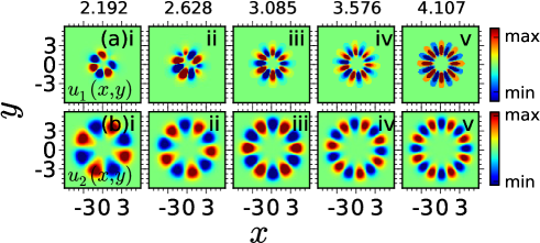
Figure 7: (Color online) Quasiparticle amplitudes corresponding to bulk excitations for the immiscible (shell structured) ⁸⁵Rb -⁸⁷Rb TBEC in space for $\alpha=1.0$. (a)i - v: Quasi particle amplitudes for species ⁸⁵Rb and (b)i - v: Quasiparticle amplitudes for species ⁸⁷Rb. Along this branch both the species have one radial nodes but the azimuthal quantum number increases with the increase of mode energy. Each set of quasiparticles starts from small values of $k$ (at left) and move towards large values of $k$ at right. In dispersion curve given in Fig. 5(a), these points are marked with empty black circles $({\color[rgb]{0,0,0}\bigcirc})$. Excitation energy for each set of $u_{1}(x,y)$ and $v_{1}(x,y)$ are highlighted at the top of the $u_{1}(x,y)$. Here $u_{1}$s and $v_{1}$s are in units of $a_{\rm osc}^{-1}$. Spatial coordinates $x$ and $y$ are measured in units of $a_{\rm osc}$.

The equilibrium density profiles for side by side density configuration are shown in Fig. 8 for different values of $\alpha$. Unlike the general trend of no preferred orientation in the side-by-side phase segregation with radially symmetric confining potential, in this case the phase segregation occurs along $y$ direction. This is appropriate since $\alpha<1.0$ indicates $\omega_{y}<\omega_{x}$ which in turn sets $y$-axis as the preferred direction for the condensate to expand more freely and at appropriate parameter regime, the phase segregation occurs along $y$. The orientation of the interface along $y$ direction occurs with the introduction of pinstripe, however small it may be.

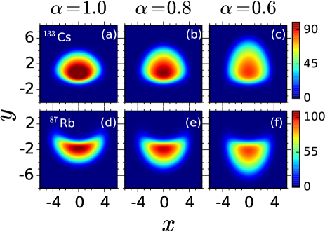
Figure 8: (Color online) Equilibrium condensate density profiles of ¹³³Cs -⁸⁷Rb TBEC for $a_{12}=220a_{0}$ at zero temperature. (a)-(c) Equilibrium density profile corresponding to ⁸⁵Rb for three different values of $\alpha$ ($\alpha$ = 1.0, 0.8, 0.5 (d)-(f)Equilibrium density profile corresponding to ⁸⁷Rb for the same three values of $\alpha$. The color bar shows the value of $n_{c}$ measured in units of $a_{\rm osc}^{-2}$. Spatial coordinates $x$ and $y$ are measured in units of $a_{\rm osc}$.

In terms of the mode evolution, the immediate consequences of phase segregation along $y$ direction is the hardening of the zero energy mode which emerges at phase separation. We observe that with the decrease in $\alpha$, the new zero energy mode regains energy and this can be attributed to the anisotropy induced stronger segregation along $y$ direction. In our earlier work, in a different system we had reported the observation of the hardening of third Goldstone mode in TBEC that emerges at phase-separation, when the confining potentials have separated trap centers Roy et al. (2015).

III.4 Excitations and dispersion relations for ¹³³Cs -⁸⁷Rb TBEC

The dispersion curves for the ¹³³Cs -⁸⁷Rb TBEC in the immiscible domain with side-by-side configuration are shown in Fig. 9. A prominent feature of the curves is that these are devoid of any discernible trends, and this is due to the lack of rotational, reflection or scaling symmetries. Some of the low-energy interface modes are identified by green circles and these are in agreement with the interface modes reported in Ref. Ticknor (2014) for TBEC with side by side configuration. To study the modes for specific $k$, we consider the modes at $k\simeq 1.8$ denoted by red solid triangles in Fig. 9 and the changes in mode structures are shown as function of $\alpha$ in Fig. 10.

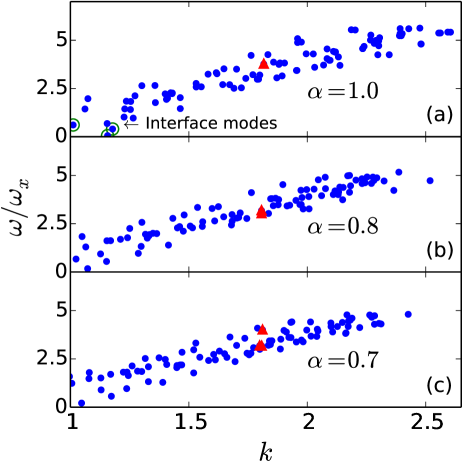
Figure 9: (Color online) (a) The dispersion relation for ¹³³Cs -⁸⁷Rb TBEC in immiscible (side by side) domain at $a_{12}$=220$a_{0}$ when $\alpha=1.0$. In this plot the dispersion curves can be broadly classified into two largely separated branches. The quasi particle amplitudes corresponding to the upper branch (near energy 6.5$\hbar\omega_{x}$) is shown in Fig. 6. For the lower branch (around energy range 1.7-2.7$\hbar\omega_{x}$), the quasi particle amplitudes is shown in Fig. 7. (b) The dispersion relation for immiscible (shell structured) ¹³³Cs -⁸⁷Rb TBEC at $a_{12}$=220$a_{0}$ when $\alpha=0.8$. (c) The dispersion relation for immiscible (shell structured) ¹³³Cs -⁸⁷Rb TBEC at $a_{12}$=220$a_{0}$ when $\alpha=0.7$. As value of $\alpha$ is reduced from 1.0 i.e., radial anisotropy makes this two branches comparatively closer to each other.

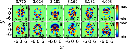
Figure 10: (Color online) Quasiparticle amplitudes for the immiscible (side by side) ¹³³Cs -⁸⁷Rb TBEC in space. (a)i - vi: Quasi particle amplitudes for species ¹³³Cs for a fixed value of $k\simeq 1.8$. (b)i - vi: Quasiparticle amplitudes for species ⁸⁷Rb for the same value of $k$. In Fig. 5 this points are marked with red solid triangles for $k=1.8$. Excitation energies corresponding to each set of $u_{1}(x,y)$ and $u_{2}(x,y)$ are mentioned at the top of each column. Here $u$s are in units of $a_{\rm osc}^{-1}$. spatial coordinates $x$ and $y$ are measured in units of $a_{\rm osc}$.

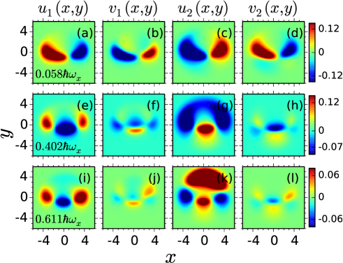
Figure 11: (Color online) Quasiparticle amplitudes corresponding to the interface modes marked as the green empty circle in Fig. 9 of the immiscible (side by side) ¹³³Cs -⁸⁷Rb TBEC for $\alpha=1.0$ . (a) - (d): Quasiparticles for the interface modes with energy 0.058$\hbar\omega_{x}$.(e)-(h): Quasiparticles for the interface modes with energy 0.402$\hbar\omega_{x}$ and (i)-(l) is those with energy 0.611$\hbar\omega_{x}$. Here $u$s are in units of $a_{\rm osc}^{-1}$. spatial coordinates $x$ and $y$ are measured in units of $a_{\rm osc}$.

Fig. 11 corresponds to the localized excitation modes of the segregated TBEC. These out-of-phase quasiparticle amplitudes describe the interface excitations and localized only at the interface separating the two condensates. The strength of quasiparticles $u_{1}(x,y)$ and $u_{2}(x,y)$ are large compared to the quasiholes denoted by $v_{1}(x,y)$ and $v_{2}(x,y)$.

IV Conclusions

In conclusion, we have characterized the low energy excitations of phase segregated TBEC in presence of radial anisotropy with the Bogoliubov–de Gennes approach. For immiscible TBEC having shell structured density profile, we have observed that the introduction of radial anisotropy modifies the structure of the interface from circular to planar. Our studies on ⁸⁵Rb -⁸⁷Rb TBEC, as an example of shell structured density, shows that the interface and bulk modes have different dispersion relations in the rotationally symmetric geometry. However, anisotropy tends to merge the the dispersion relations. For the side by side geometry the effect of the radial anisotropy manifest through the breaking of rotational symmetry and interface orients along minor axis. This follows from energy minimization through shorter interface geometry. For this case we have chosen ¹³³Cs -⁸⁷Rb TBEC as an example and demonstrate that the lack of symmetry lead to a dispersion curve which is devoid of any discernible trends. Furthermore, the effect of the anisotropy on the structure of the quasiparticles for these two systems are examined. One important difference between the two in the immiscible domain is, the TBEC with side by side geometry has interface modes as the lowest-energy modes. Whereas for the shell structured density profile the interface modes relatively higher energies.

Appendix A

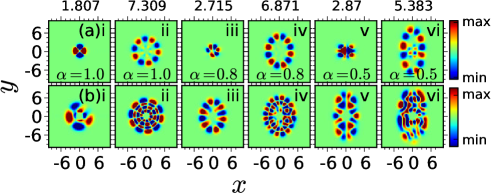
Figure 12: (Color online) Quasiparticle amplitudes for the immiscible (shell structured) ⁸⁵Rb -⁸⁷Rb TBEC in space for a particular $k\sim 1.85$. The corresponding mode energies are marked with maroon triangle $({\color[rgb]{0,0,0}\blacktriangle})$ in Fig. 5. (a)i- vi: Quasi particle amplitudes for species ⁸⁵Rb. (b)i - vi: Quasiparticle amplitudes for species ⁸⁷Rb. (ii),(iv),(vi) in both the row (a) and (b) represent the interface modes. Whereas (i),(iii),(v) in row (a) denote the bulk excitations for ⁸⁵ Rb and those in row (b) are bulk excitations of ⁸⁷Rb. Each set of quasiparticles start from $\alpha=1.0$ and move towards $\alpha=0.5$. Excitation energy corresponding to each set of $u_{1}(x,y)$ and $u_{2}(x,y)$ are mentioned at the top of each column. Here $u$s are in units of $a_{\rm osc}^{-1}$. spatial coordinates $x$ and $y$ are measured in units of $a_{\rm osc}$.

To compare the structure of the interface and bulk modes at higher momenta, we consider modes with $k\sim 1.85$ and plot of the quasiparticle amplitudes are shown in Fig. 12. The plots correspond to the modes marked with maroon triangle $({\color[rgb]{0,0,0}\blacktriangle})$ in the dispersion curve in Fig. 5. In Fig. 12, the plots in the top (bottom) row are the quasiparticles for ⁸⁵Rb (⁸⁷Rb). Among these the plots labeled with even number (ii, iv, and vi) are the interface modes and the other are the bulk modes. Comparing the energies, top label in the plots, the interface modes have energies which are more than double of the bulk modes with similar $k$, and this is due to the localized nature of the interface modes. The important trend discernible is the decrease in mode energies, for the same $k$, with the decrease in $\alpha$. This is on account of the reduced trapping frequency along the $y$-axis. The other effect of the anisotropy is the deformation of the interface quasiparticle particle when the interface changes from circular to planer geometry. The appearance of the nonzero values in the central region in Fig. 12(a)(vi) is a The other noticeable trend is the drastic transformation in the quasiparticle amplitudes of ⁸⁷Rb, which lies at the periphery, with decrease of $\alpha$. Compared to which the quasiparticle amplitudes of ⁸⁵Rb, which occupies the core region, the changes in their structure is not large.

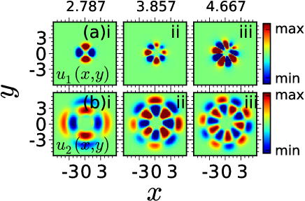
Figure 13: (Color online) Quasiparticle amplitudes corresponding to bulk excitations with relatively large-$k$ for the immiscible (shell structured) ⁸⁵Rb -⁸⁷Rb TBEC in space for $\alpha=1.0$. (a)i - iii: Quasi particle amplitudes for species ⁸⁵Rb which are composed of one radial nodes and $m$ varying with mode energies. (b)i - iii: Quasiparticle amplitudes for species ⁸⁷Rb with two radial nodes and $m$ varying with mode energies like other species. In dispersion curves shown in Fig. 5(a), these modes are marked with orange square $({\color[rgb]{0,0,0}\blacksquare})$. Excitation energy for each set of $u_{1}(x,y)$ and $v_{1}(x,y)$ are highlighted at the top of the $u_{1}(x,y)$ Here $u_{1}$s and $v_{1}$s are in units of $a_{\rm osc}^{-1}$. Spatial coordinates $x$ and $y$ are measured in units of $a_{\rm osc}$.

A selected set of higher energy bulk modes, lower branch in the dispersion curve, with larger number of radial nodes are shown in Fig. 13. The modes chosen are marked with orange square $({\color[rgb]{0,0,0}\blacksquare})$ in the dispersion curve which is shown in Fig. 5. Like in the previous figures, $u_{1}(x,y)$ denotes the quasiparticles for ⁸⁵Rb atoms and these are given in Fig. 5(a)(i-iii). Similarly, $u_{2}(x,y)$ correspond to those for ⁸⁷Rb and are shown in 5(b)(i-iii). The notable feature is that the quasiparticles of ⁸⁵Rb have only one radial node whereas those of ⁸⁷Rb have two radial nodes.

References

- Davis et al. (1995) K. B. Davis, M. O. Mewes, M. R. Andrews, N. J. van Druten, D. S. Durfee, D. M. Kurn, and W. Ketterle, Phys. Rev. Lett. 75, 3969 (1995).
- Anderson et al. (1995) M. H. Anderson, J. R. Ensher, M. R. Matthews, C. E. Wieman, and E. A. Cornell, Science 269, 198 (1995).
- Roy et al. (2015) A. Roy, S. Gautam, and D. Angom, Eur. Phys. J. Spec. Top. 224, 571 (2015).
- Roy and Angom (2016) A. Roy and D. Angom, New J. Phys. 18, 083007 (2016).
- Timmermans (1998) E. Timmermans, Phys. Rev. Lett. 81, 5718 (1998).
- Pu and Bigelow (1998) H. Pu and N. P. Bigelow, Phys. Rev. Lett. 80, 1134 (1998).
- Ho and Shenoy (1996) T.-L. Ho and V. B. Shenoy, Phys. Rev. Lett. 77, 3276 (1996).
- Gautam and Angom (2010) S. Gautam and D. Angom, J. Phys. B 43, 095302 (2010).
- Mertes et al. (2007) K. M. Mertes, J. W. Merrill, R. Carretero-González, D. J. Frantzeskakis, P. G. Kevrekidis, and D. S. Hall, Phys. Rev. Lett. 99, 190402 (2007).
- Papp and Wieman (2006) S. B. Papp and C. E. Wieman, Phys. Rev. Lett. 97, 180404 (2006).
- Papp et al. (2008) S. B. Papp, J. M. Pino, and C. E. Wieman, Phys. Rev. Lett. 101, 040402 (2008).
- McCarron et al. (2011) D. J. McCarron, H. W. Cho, D. L. Jenkin, M. P. Köppinger, and S. L. Cornish, Phys. Rev. A 84, 011603(R) (2011).
- Pethick and Smith (2008) C. Pethick and H. Smith, Bose-Einstein Condensation in Dilute Gases (Cambridge University Press, New York, 2008).
- Wilson et al. (2010) R. M. Wilson, S. Ronen, and J. L. Bohn, Phys. Rev. Lett. 104, 094501 (2010).
- Bisset and Blakie (2013) R. N. Bisset and P. B. Blakie, Phys. Rev. Lett. 110, 265302 (2013).
- Blakie et al. (2012) P. B. Blakie, D. Baillie, and R. N. Bisset, Phys. Rev. A 86, 021604 (2012).
- Ticknor et al. (2011) C. Ticknor, R. M. Wilson, and J. L. Bohn, Phys. Rev. Lett. 106, 065301 (2011).
- Ticknor (2014) C. Ticknor, Phys. Rev. A 89, 053601 (2014).
- Klaiman et al. (2017) S. Klaiman, R. Beinke, L. S. Cederbaum, A. I. Streltsov, and O. E. Alon, arXiv:1709.04223v1 (2017).
- Petrov et al. (2000) D. S. Petrov, M. Holzmann, and G. V. Shlyapnikov, Phys. Rev. Lett. 84, 2551 (2000).
- Griffin (1996) A. Griffin, Phys. Rev. B 53, 9341 (1996).
- Ticknor (2013) C. Ticknor, Phys. Rev. A 88, 013623 (2013).
- Roy et al. (2014) A. Roy, S. Gautam, and D. Angom, Phys. Rev. A 89, 013617 (2014).
- Pal et al. (2017) S. Pal, A. Roy, and D. Angom, J. Phys B. 50, 195301 (2017).
- Kohn (1961) W. Kohn, Phys. Rev. 123, 1242 (1961).
- Fetter and Rokhsar (1998) A. L. Fetter and D. Rokhsar, Phys. Rev. A 57, 1191 (1998).
- Al-Jibbouri and Pelster (2013) H. Al-Jibbouri and A. Pelster, Phys. Rev. A 88, 033621 (2013).
- Nguyen and Peeters (2010) N. T. T. Nguyen and F. M. Peeters, J. Phys.: Conf. Ser. 245, 012031 (2010).
- Neely et al. (2010) T. W. Neely, E. C. Samson, A. S. Bradley, M. J. Davis, and B. P. Anderson, Phys. Rev. Lett. 104, 160401 (2010).
- Cornish et al. (2000) S. L. Cornish, N. R. Claussen, J. L. Roberts, E. A. Cornell, and C. E. Wieman, Phys. Rev. Lett. 85, 1795 (2000).
- Suthar et al. (2015) K. Suthar, A. Roy, and D. Angom, Phys. Rev. A 91, 043615 (2015).
- Suthar and Angom (2016) K. Suthar and D. Angom, Phys. Rev. A 93, 063608 (2016).
- Lercher et al. (2011) A. Lercher, T. Takekoshi, M. Debatin, B. Schuster, R. Rameshan, F. Ferlaino, R. Grimm, and H.-C. Nägerl, Eur. Phys. J. D 65, 3 (2011).