Metastability of one-dimensional, non-reversible diffusions with periodic boundary conditions.

Abstract.

We consider small perturbations of a dynamical system on the one-dimensional torus. We derive sharp estimates for the pre-factor of the stationary state, we examine the asymptotic behavior of the solutions of the Hamilton-Jacobi equation for the pre-factor, we compute the capacities between disjoint sets, and we prove the metastable behavior of the process among the deepest wells following the martingale approach. We also present a bound for the probability that a Markov process hits a set before some fixed time in terms of the capacity of an enlarged process.

1. Introduction

Variational formulae for the capacity between two sets have been derived recently in the context of continuous time Markov chains and diffusions [9, 19, 14]. These formulae were used to prove the metastable behavior of asymmetric condensing zero-range processes [11], random walks in a potential field [15], mean field Potts model [16], and to derive the Eyring-Kramers formula for the transition time of non-reversible diffusions [14].

To estimate the capacity through the variational formulae alluded to above, one needs to know explicitly the stationary state. This property is shared by all the dynamics mentioned in the previous paragraph, where the invariant measures are the equilibrium states of the reversible version of the dynamics. Usually, however, the stationary states of non-reversible Markovian dynamics are not known explicitly.

It is possible, nonetheless, to derive through dynamical large deviations methods a formula for the quasi-potential of non-reversible dynamics and estimates for the stationary state with exponentially small errors [8]. A natural development of this approach consists in using potential theory to get sharper bounds of the stationary state, that is, to provide precise estimates for the first-order term in the expansion of the quasi-potential, the so-called pre-factor.

For one-dimensional diffusion processes with periodic boundary conditions,

$$dX_{\epsilon}(t)\;=\;b(X_{\epsilon}(t))\,dt\;+\;\sqrt{2\epsilon}\,dW_{t}\;,$$ (1.1)

where $b:{\mathbb{T}}\to{\mathbb{R}}$ is a smooth drift, $\epsilon>0$ a small parameter and $W_{t}$ the Brownian motion on the one-dimensional torus ${\mathbb{T}}=[0,1)$, one may derive sharp estimates for the pre-factor due to an explicit formula for the stationary state obtained by Faggionato and Gabrielli [7]. This estimate and the precise bounds for the capacity between two wells constitute the first main result of the article.

The pre-factor of the stationary state solves a Hamilton-Jacobi equation. We take advantage of the explicit formulae to examine the asymptotic behavior of the solution of the Hamilton-Jacobi equation in the hope that these results might give some insight on the behavior of the pre-factor in higher dimensions.

The second main result of this article provides an extension to diffusion processes of the martingale approach proposed in [1, 2, 3] to derive the metastable behavior of Markov chains. The main difficulty in applying this method to diffusions lies in the fact that the martingale approach requires an analysis of the trace of the process on the wells. While for Markov chains the trace process is still a Markov chain [with long range jumps], for diffusions the trace becomes a singular diffusion with jumps along the boundary of the wells, a dynamics very different from the original one and difficult to analyze.

We present in this article an entirely new approach inspired by results in partial differential equations obtained by Evans, Tabrizian and Seo, Tabrizian [6, 18]. Here is the idea. Denote by ${\mathscr{E}}_{i}$, $1\leq i\leq n$, the wells, and let $G$ be a function defined on the entire space and which is constant [with possibly different values] in each well. Denote by $L_{\epsilon}$ the generator and by $F_{\epsilon}$ the solution of the Poisson equation $L_{\epsilon}F_{\epsilon}=G$. Assume that for all such functions $G$ the solution $F_{\epsilon}$ is uniformly bounded and is asymptotically constant in each well. We prove in Section 7 that the convergence in law of the projection of the trace process on the wells follows from the previous property of the solutions of the Poisson equation.

This new way of deriving the metastable behavior of a Markov chain is applied here to small perturbations of the dynamical system (1.1). It also provides the first example where the reduced chain, which describes the asymptotic dynamics among the wells, is a irreducible, non-reversible Markov chain.

The third main result of the article consists in a bound on the probability that the hitting time of a set is less than or equal to a constant in terms of capacities. In view of the variational formulae for the capacity, this result provides a general method to obtain upper bounds for the probability of an event which appears in many different contexts.

We conclude this introduction with some historical remarks and a description of the article. The convergence of the order parameter, in the sense of finite-dimensional distributions, of small perturbations by reversible Gaussian noises of dynamical systems has been proved by Sugiura in [20]. Imkeller and Pavlyukevich obtained a similar result in one-dimension when the Brownian motion is replaced by a Lévy process. More recently, Bouchet and Reygner [4] derived a formula for the transition time between two wells for non-reversible diffusions. A rigorous proof of this result is still an open problem.

The paper is organized as follows. In Section 2, we introduce the model and the main assumptions on the drift $b$. In Section 3, we present the main results of the article in the case of two wells. In Section 4, we introduce the notion of valleys and landscapes used throughout the article. In Sections 5 and 6, we derive sharp asymptotic estimates for the pre-factor and for the capacity between two wells. In Section 7, we prove the metastable behavior of the process by showing that the projection of the trace process on the wells converges in an appropriate time scale to a finite-state Markov chain. In Section 8, we prove a bound on the probability that a certain set is attained before a fixed time in terms of the capacities of an enlarged process. Finally, in Section 9, we prove that the solutions of certain Poisson equations are asymptotically constant on the wells.

2. The model

We introduce in this section the model, the main assumptions and known results.

2.1. The diffusion process. Let ${\mathbb{T}}=[0,1)$ be the one-dimensional torus of length $1$. Consider a continuous vector field $b:{\mathbb{T}}\to{\mathbb{R}}$. Throughout this article, we assume that $b$ fulfills the following conditions:
(H1) The closed set $\{\theta\in{\mathbb{T}}:b(\theta)=0\}$ has a finite number of connected components, denoted by $I_{j}=[l_{j},r_{j}]$, $1\leq j\leq p$, for $0<l_{1}\leq r_{1}<l_{2}\leq\cdots<l_{p}\leq r_{p}<1$. Some of these intervals may be degenerate, as we do not exclude the possibility that $l_{j}=r_{j}$.
(H2) $b$ is of class $C^{2}$ in the set ${\mathbb{T}}\setminus I$, where $I=\cup_{1\leq j\leq p}\,I_{j}$.
(H3) If $(c,d)$ is a connected component of ${\mathbb{T}}\setminus I$, then $b^{\prime}(c+)\not=0$ and $b^{\prime}(d-)\not=0$. When the interval $[l_{j},r_{j}]$ is degenerate, $l_{j}=r_{j}$, the left and right derivatives of $b$ at $r_{j}$ may be different: it may happen that $b^{\prime}(r_{j}-)\not=b^{\prime}(r_{j}+)$. However, both right and left derivatives do not vanish.

The generator of the diffusion (1.1), denoted by $L_{\epsilon}$, is given by

$$(L_{\epsilon}f)(\theta)\;=\;b(\theta)f^{\prime}(\theta)\;+\;\epsilon\,f^{\prime\prime}(\theta)\;.$$

If the average drift vanishes,

$$\int_{{\mathbb{T}}}b(\theta)\,d\theta\;=\;0\;,$$

there exists a potential $U:{\mathbb{T}}\to{\mathbb{R}}$ such that $b(\theta)=-\,U^{\prime}(\theta)$. In this case the stationary measure is given by $Z^{-1}_{\epsilon}\exp\{-U(\theta)/\epsilon\}\,d\theta$ for a suitable normalization factor $Z_{\epsilon}^{-1}$ and the process is reversible with respect to this measure.

Assume, from now on, that

$$B\;:=\;\int_{{\mathbb{T}}}b(\theta)\,d\theta\;>\;0\;,$$ (2.1)

so that the process $X_{\epsilon}(t)$ is non-reversible. In [7], the stationary measure of this process has been explicitly computed. Regard $b$ as an $1$-periodic function on ${\mathbb{R}}$. Let $S:{\mathbb{R}}\to{\mathbb{R}}$ be the function given by

$$S(x)\;=\;-\int_{0}^{x}b(z)\,dz\;,$$ (2.2)

and let $\pi_{\epsilon}$, $m_{\epsilon}:{\mathbb{R}}\to{\mathbb{R}}_{+}$ be given by

$$\pi_{\epsilon}(x)\;=\;\int_{x}^{x+1}e^{[S(y)-S(x)]/\epsilon}\,dy\;,\quad m_{\epsilon}(x)\;=\;\frac{1}{c(\epsilon)}\,\pi_{\epsilon}(x)\;,$$ (2.3)

where $c(\epsilon)$ is the normalizing constant which turns $m_{\epsilon}$ the density of a probability measure on ${\mathbb{T}}$. Indeed, $\pi_{\epsilon}$, $m_{\epsilon}$ are $1$-periodic and can be considered as defined on ${\mathbb{T}}$. By [7], the measure $\mu_{\epsilon}(d\theta)=m_{\epsilon}(\theta)\,d\theta$ on ${\mathbb{T}}$ is the stationary state of the diffusion (1.1).

2.2. The quasi-potential. Let $z:{\mathbb{R}}\to{\mathbb{R}}$ be the function which indicates the position of the farthest maxima of $S$ to the right: $z(x)=z_{x}$ is the largest point in $[x,\infty)$ at which a maximum of the set $\{S(y):y\geq x\}$ is attained. More precisely,
(a) $\displaystyle S(z_{x})\;=\;\max\{S(y):y\geq x\}$,
(b) If $y\geq x$ and $S(y)=S(z_{x})$, then $y\leq z_{x}$.

Note that, for all $x\in{\mathbb{R}}$, $z(x)$ not only exists but also satisfies $z(x)\in[x,x+1)$ because $S(y+1)=S(y)-B<S(y)$. Moreover, $z_{x}$ is a local maximum of $S$ if $z_{x}\not=x$. In this case, $b(z_{x})=-S^{\prime}(z_{x})=0$.

Let $\widehat{V}:{\mathbb{R}}\to{\mathbb{R}}$ be given by

$$\widehat{V}(x)\;=\;S(x)\;-\;S(z_{x})\;.$$

Since $S(y+k)=S(y)-kB$ for $y\in{\mathbb{R}}$, $k\in{\mathbb{Z}}$, $z(x+k)=z(x)+k$. In particular, $\widehat{V}(x+1)=\widehat{V}(x)$, so that $\widehat{V}$ is a $1$-periodic function and can be considered as defined on the torus ${\mathbb{T}}$. By [7, Proposition 2.1], $\widehat{V}$ is the quasi-potential associated to the diffusion (1.1), and by [7, Theorem 2.4] it is a viscosity solution of the Hamilton-Jacobi equation associated to the Hamiltonian $H(x,p)=p[p-b(x)]$.

3. Main result: Two stable points

We present in this section the main results of the article in the case, illustrated in Figure 1, where the drift $b$ is smooth and the dynamical system $dX(t)=b(X(t))\,dt$ exhibits two stable equilibria and two unstable ones.

In addition to the conditions (H1-H3), we shall assume in this section that

(H0) The drift $b$ is smooth and the set $\{\theta\in{\mathbb{T}}:b(\theta)=0\}$ consists of four points.

Condition (H0) is not needed in the proofs of the results presented in this article. It is assumed in this section because it simplifies significantly the notation and the statement of the results, helping the reader to access the content of the article. Further assumptions will be formulated along the section.

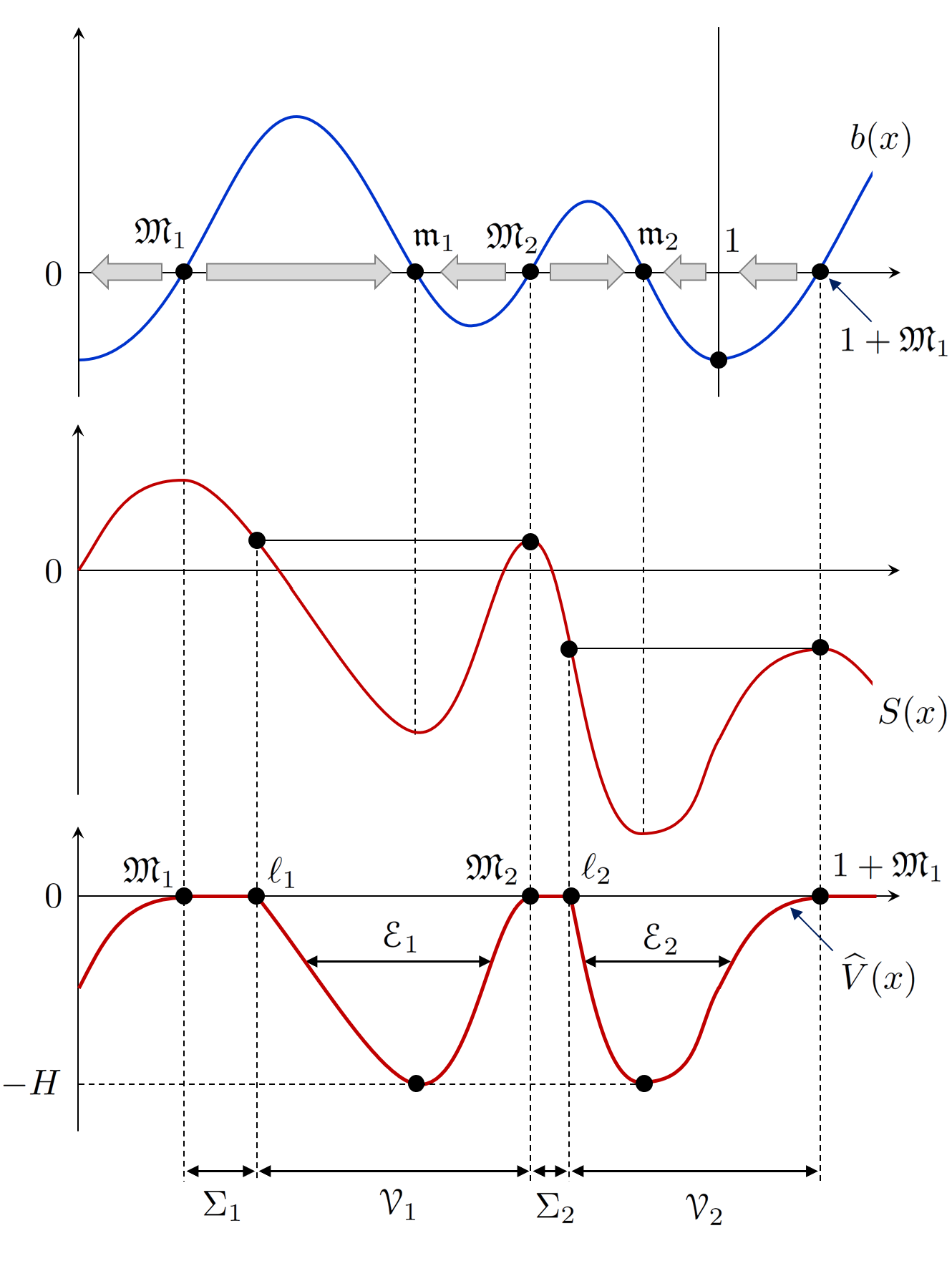
Figure 1. The graphs of $b$, $S$ and $\widehat{V}$. In the first graph, the gray arrows represent the direction of the drift in the dynamical system $dX(t)=b(X(t))\,dt$. Thus, ${\mathfrak{m}}_{1}$ and ${\mathfrak{m}}_{2}$ are stable equilibria, and ${\mathfrak{M}}_{1}$ and ${\mathfrak{M}}_{2}$ are unstable equilibria. The existence of two stable equilibria separated by unstable one implies a metastable behavior of the perturbed dynamics (1.1).

3.1. Notation. By assumptions (H0) and (H3), $S(\cdot)$ has two local maxima ${\mathfrak{M}}_{1},\,{\mathfrak{M}}_{2}$ and two local minima ${\mathfrak{m}}_{1},\,{\mathfrak{m}}_{2}$. Without loss of generality, we assume that $0<{\mathfrak{M}}_{1}<{\mathfrak{m}}_{1}<{\mathfrak{M}}_{2}<{\mathfrak{m}}_{2}<1$, and that that $S({\mathfrak{M}}_{1})>S({\mathfrak{M}}_{2})>S({\mathfrak{M}}_{3})$, where we adopted the convention that ${\mathfrak{M}}_{3}=1+{\mathfrak{M}}_{1}$. We refer to Figure 1 for the graphs of $b(\cdot),\,S(\cdot)$ and $\widehat{V}(\cdot)$.

For each $i=1,\,2$, let $\ell_{i}=\inf\{x>{\mathfrak{M}}_{i}:S(x)=S({\mathfrak{M}}_{i+1})\}$ and set

$$\Sigma_{i}\;=\;({\mathfrak{M}}_{i},\,\ell_{i})\;,\;\;{\mathscr{V}}_{i}\;=\;(\ell_{i},\,{\mathfrak{M}}_{i+1})\;,\;\;i=1,\,2\;.$$

Note that ${\mathscr{V}}_{2}$ can be regarded as the subset of ${\mathbb{T}}$ given by $(\ell_{i},\,1]\cup(0,\,{\mathfrak{M}}_{1})$. These notation will be comprehensively extended to a general drift $b$ in Section 4. Note that for $x\in\Sigma_{1}\cup\Sigma_{2}$, one has that $z(x)=x$ and hence $\widehat{V}(x)=0$ (cf. Figure 1). Thus, the sets $\Sigma_{i}$, $i=1,\,2$, represent the saddle intervals between two valleys ${\mathscr{V}}_{1}$ and ${\mathscr{V}}_{2}$. The notion of valley is extended to the one of landscape in Section 4 to handle more general situations. The depth of the valleys ${\mathscr{V}}_{1}$ and ${\mathscr{V}}_{2}$ are $-\,\widehat{V}({\mathfrak{m}}_{1})$ and $-\,\widehat{V}({\mathfrak{m}}_{2})$, respectively. Assume that

$$\widehat{V}({\mathfrak{m}}_{1})\;=\;\widehat{V}({\mathfrak{m}}_{2})\;=\;-H\;,$$ (3.1)

so that the depth of the two valleys coincide. This assumption is not necessary for the results below, but without it the results become trivial and can easily be deduced from the argument.

For $i=1,\,2$, let ${\mathscr{E}}_{i}=[e_{i}^{-},\,e_{i}^{+}]\subseteq{\mathscr{V}}_{i}$ be such that $\widehat{V}({\mathfrak{m}}_{i})<\widehat{V}(e_{i}^{-})=\widehat{V}(e_{i}^{+})<0$ so that ${\mathfrak{m}}_{i}\in{\mathscr{E}}_{i}$. The set ${\mathscr{E}}_{i}$ represents the metastable well around the stable point ${\mathfrak{m}}_{i}$.

3.2. Sharp asymptotics for the pre-factor. The first main result of the article provides a sharp estimate of the stationary state. Write $m_{\epsilon}$ as

$$m_{\epsilon}(\theta)\;=\;F_{\epsilon}(\theta)\,e^{-V(\theta)/\epsilon}\;,$$

where $V(\theta)=\widehat{V}(\theta)+H$. The function $F_{\epsilon}(\cdot)$ is called the pre-factor. Its behavior as $\epsilon\to 0$ plays a fundamental role in the estimation of the capacity between two wells, which is one of the crucial steps in the proof of the metastable behavior of a Markov chain. Such a result is still open in the non reversible context except in the trivial case where the pre-factor is constant. The first main result of this article provides an expansion in $\epsilon$ of the pre-factor. For $i=1$, $2$, let

$$\sigma({\mathfrak{m}}_{i})\;=\;\sqrt{\frac{2\pi}{-b^{\prime}({\mathfrak{m}}_{i})}}\;,\quad\omega({\mathfrak{M}}_{i})\;=\;\sqrt{\frac{2\pi}{b^{\prime}({\mathfrak{M}}_{i})}}\;,\quad Z\;=\;\sum_{j=1}^{2}\sigma({\mathfrak{m}}_{j})\,\omega({\mathfrak{M}}_{j+1})\;.$$

Theorem 3.1.

Under the assumptions (H0-H3),

1. (Pre-factor on valleys) for all $x\in{\mathscr{V}}_{i}$, $i=1,\,2$,

   $$F_{\epsilon}(x)\;=\;\big{[}1+o(1)\big{]}\,\frac{\omega({\mathfrak{M}}_{i+1})}{Z\,\sqrt{\epsilon}}$$

   where $o(1)\rightarrow 0$ as $\epsilon\rightarrow 0$ uniformly on ${\mathscr{V}}_{1}\cup{\mathscr{V}}_{2}$.

2. (Pre-factor on saddle intervals) for all $x\in\Sigma_{1}\cup\Sigma_{2}$,

   $$F_{\epsilon}(x)\;=\;\big{[}1+o(1)\big{]}\,\frac{1}{Z\,b(x)}\;.$$

   where $o(1)\rightarrow 0$ as $\epsilon\rightarrow 0$ for all $x\in\Sigma_{1}\cup\Sigma_{2}$.

The general case, without assumption(H0), is presented in Propositions 5.2 and 5.3. Note the difference in the scaling factor in parts (1) and (2). This difference is explained along with a connection to the Hamilton-Jacobi equation for $F_{\epsilon}$ in Subsection 5.5. The scaling difference of the pre-factor indicates that its asymptotic analysis in higher dimension may be a difficult problem.

3.3. Metastable behavior. We turn to the metastable behavior of the diffusion $X_{\epsilon}(t)$ between the valleys ${\mathscr{E}}_{1}$ and ${\mathscr{E}}_{2}$. Let $\widehat{X}_{\epsilon}(t):=X_{\epsilon}(e^{H/\epsilon}t)$ be the speeded-up process. As in the approach developed in [1, 2], we define the metastable behavior of the diffusion as the convergence of the projection of the trace process.

To define the trace process of $\widehat{X}_{\epsilon}(t)$ on ${\mathscr{E}}={\mathscr{E}}_{1}\cup{\mathscr{E}}_{2}$, let

$$T_{{\mathscr{E}}}(t)\;=\;\int_{0}^{t}\chi_{{\mathscr{E}}}(\widehat{X}_{\epsilon}(s))\,ds\;,\quad S_{{\mathscr{E}}}(t)\;=\;\sup\{s\geq 0:T_{{\mathscr{E}}}(s)\leq t\}\;.$$

The process $Y_{\epsilon}(t)=\widehat{X}_{\epsilon}(S_{{\mathscr{E}}}(t))$ is called the trace of the process $\widehat{X}_{\epsilon}$ on ${\mathscr{E}}$. Informally, one obtains a trajectory of $Y_{\epsilon}(t)$ from $\widehat{X}_{\epsilon}(t)$ by deleting the excursion of $\widehat{X}_{\epsilon}$ outside ${\mathscr{E}}$. In Subsection 7.4, we show that $Y_{\epsilon}(\cdot)$ is a Markov process on ${\mathscr{E}}$ with respect to a suitable filtration. Let $\Psi:{\mathscr{E}}\rightarrow\{1,\,2\}$ be the projection defined by $\Psi(x)=\chi_{{\mathscr{E}}_{1}}(x)+2\chi_{{\mathscr{E}}_{2}}(x)$. Clearly, ${\boldsymbol{x}}_{\epsilon}(t)=\Psi(Y_{\epsilon}(t))$ takes values in the set $\{1,\,2\}$, and represents the valley visited by the process $Y_{\epsilon}(t)$. Following [1, 2], we shall say that the process $X_{\epsilon}(t)$ is metastable in the time-scale $e^{H/\epsilon}$ if ${\boldsymbol{x}}_{\epsilon}(\cdot)$ converges to a Markov chain on $\{1,\,2\}$, and if the process $\widehat{X}_{\epsilon}(t)$ remains outside ${\mathscr{E}}$ for a negligible amount of time.

The method developed in [1, 2, 3] provides a robust way to establish these results. Moreover, it has been shown in [13] that under some mild extra assumptions the metastability as stated above entails the convergence of the finite-dimensional distributions of the projections of $\widehat{X}_{\epsilon}(t)$.

This approach to metastability was successfully enforced in the context of Markov chains. Its extension to diffusions, such as the one considered in the current paper, faced a major difficulty due to the singular behavior of the trace process $Y_{\epsilon}(t)$ at the boundary of ${\mathscr{E}}$. In this paper, we propose a new way of establishing the convergence of the projection of the trace process based on results from the theory of partial differential equations (cf. [6, 18]). This is the content of Sections 7 and 9.

Let

$$R(1,\,2)\;=\;\frac{1}{\sigma({\mathfrak{m}}_{1})\,\omega({\mathfrak{M}}_{2})}\;,\quad R(2,\,1)\;=\;\frac{1}{\sigma({\mathfrak{m}}_{2})\,\omega({\mathfrak{M}}_{1})}\;,$$

and consider the Markov chain ${\boldsymbol{X}}(t)$ on $\{1,\,2\}$ with generator given by

$$({\boldsymbol{L}}f)(i)\;=\;R(i,\,j)\left[F(j)-F(i)\right]\;,\quad\{i,\,j\}\,=\,\{1,\,2\}\;.$$

Let ${\boldsymbol{Q}}_{j}$, $j=1,\,2$, be the law of the Markov chain ${\boldsymbol{X}}(t)$ starting from $j$.

Theorem 3.2.

Fix $j\in\{1,\,2\}$, $\theta_{0}\in{\mathscr{E}}_{j}$ and suppose that $X_{\epsilon}(0)=\theta_{0}$ for all $\epsilon>0$. Then, the law of the process $Y_{\epsilon}(\cdot)$ converges to ${\boldsymbol{Q}}_{j}$ as $\epsilon\to 0$.

The general version of this result is presented in Theorem 7.3. Although, under (H0), the process ${\boldsymbol{X}}(t)$ is reversible with respect to its invariant distribution, this is no longer true in the general setting. Actually, Theorem 7.3 provides the first example of a dynamics whose asymptotic evolution is described by a non-reversible and irreducible Markov chain.

The proof of Theorem 3.2 is divided in two parts. We have first to establish the tightness of the process ${\boldsymbol{x}}_{\epsilon}(t)$ (cf. Section 7.5). The core step in the proof of this result is an estimation of the escape time from a metastable well. For this purpose we establish a general inequality, presented in Proposition 8.1, which bounds the hitting time of a set in terms of a capacity which can be easily estimated through the variational formulae for the capacity. We believe that this inequality, the third main result of the article, can be useful in numerous different contexts.

The second part of the proof consists in the characterization of the limit point. This part is based on the analysis of the solution of a certain Poisson equation (cf. Proposition 9.1). This sort of analysis has been carried out in [6, 18] for reversible diffusions based on ideas from PDEs.

4. Valleys and landscapes

Figure 2. This figure represents the graph on the interval $[-\delta,1+\delta]$ of a functions $S:{\mathbb{R}}\to{\mathbb{R}}$ associated by (2.2) to a vector field $b$ defined on the torus ${\mathbb{T}}$. In this example, the set $\{\theta\in{\mathbb{T}}:b(\theta)=0\}$ has $p=10$ connected components. There are $q=4$ local maxima, and ${\boldsymbol{m}}=2$ landscapes indicated in brown. The landscape $\Lambda_{1}$ has two valleys represented in blue, while the landscape $\Lambda_{2}$ has only $1$ valley. The two saddle intervals $\Sigma_{1}$, $\Sigma_{2}$ are displayed in red.

We introduce in this section the notion of valleys and landscapes which play an important role in the description of the quasi-potential $\widehat{V}$.

Let ${\mathscr{A}}_{k}=[{\mathfrak{M}}^{-}_{k},{\mathfrak{M}}^{+}_{k}]$, $1\leq k\leq q$, $q\geq 0$, (resp. ${\mathscr{U}}_{j}=[{\mathfrak{m}}^{-}_{j},{\mathfrak{m}}^{+}_{j}]$, $1\leq j\leq q^{\prime}$, $q^{\prime}\geq 0$) be the sub-intervals of $[0,1)$ where $S$ assumes a local maximum (resp. minimum). For the local maxima, this means that $b$ vanishes on each interval $[{\mathfrak{M}}^{-}_{k},{\mathfrak{M}}^{+}_{k}]$ and that $b^{\prime}({\mathfrak{M}}^{+}_{k})>0$, $b^{\prime}({\mathfrak{M}}^{-}_{k})>0$. Similar relations hold for the intervals where $S$ attains a local minimum. Note that $q$, $q^{\prime}$ might be equal to $0$. The set ${\mathscr{A}}_{1}$ is represented in Figure 2.

Since each local maxima is succeeded by a local minima, $q^{\prime}$ must be equal to $q$. The intervals ${\mathscr{A}}_{k}$, ${\mathscr{U}}_{k}$ might be reduced to points, and they are supposed to be ordered in the sense that $0\leq{\mathfrak{M}}^{-}_{1}\leq{\mathfrak{M}}^{+}_{1}<{\mathfrak{m}}^{-}_{1}\leq{\mathfrak{m}}^{+}_{1}<{\mathfrak{M}}^{-}_{2}<\cdots<{\mathfrak{M}}^{+}_{q}<{\mathfrak{m}}^{-}_{q}\leq{\mathfrak{m}}^{+}_{q}<1$. For $m\in{\mathbb{Z}}$, $1\leq j\leq q$, let ${\mathfrak{M}}^{\pm}_{j+mq}=m+{\mathfrak{M}}^{\pm}_{j}$, ${\mathfrak{m}}^{\pm}_{j+mq}=m+{\mathfrak{m}}^{\pm}_{j}$.

Observe that

$$z(x)\;=\;x\;\;\text{or}\;\;z(x)\;\in\;\big{\{}{\mathfrak{M}}^{+}_{k}:{\mathfrak{M}}^{+}_{k}\,>\,x\big{\}}\;.$$ (4.1)

Indeed, if $z(x)\not=x$, $z(x)$ must be greater than $x$ and $z(x)$ must be the right endpoint of an interval where $S$ attains a local maximum.

If $q=0$, the diffusion $X_{\epsilon}(t)$ has a nonnegative drift. In this case, $S$ is a non-increasing function and $S(x)=S(z_{x})$ for all $x\in{\mathbb{R}}$ so that the quasi-potential vanishes, $\widehat{V}\equiv 0$. Conversely, if $\widehat{V}\equiv 0$, $S(z_{x})=S(x)$ for all $x$, which implies that $S$ has no local minima. Hence,

$$\widehat{V}\equiv 0\quad\text{if and only if}\quad b\;\geq\;0\quad\text{if and only if}\quad q\;=\;0\;.$$

Assume from now on that $q\geq 1$. Consider a local maximum ${\mathfrak{M}}^{+}_{k}$ such that

$$z({\mathfrak{M}}^{+}_{k})\;=\;{\mathfrak{M}}^{+}_{k}\;.$$ (4.2)

There is at least one maximum which comply with this condition: if ${\mathfrak{M}}^{+}_{1}$ does not fulfill it, then $z({\mathfrak{M}}^{+}_{1})$ does. In Figure 2, ${\mathfrak{M}}^{+}_{1}$, ${\mathfrak{M}}^{+}_{4}$ are the maxima which satisfy this condition.

Denote by ${\boldsymbol{m}}$ the number of local maxima which satisfy condition (4.2), and represent them by ${\mathfrak{L}}^{\pm}_{n}={\mathfrak{M}}^{\pm}_{j(n)}$, $1\leq n\leq{\boldsymbol{m}}$, for some sequence $1\leq j(1)<\cdots<j({\boldsymbol{m}})\leq q$. As ${\boldsymbol{m}}\geq 1$ and ${\boldsymbol{m}}\leq q$, we have that $0\leq{\mathfrak{L}}^{+}_{1}<\dots<{\mathfrak{L}}^{+}_{{\boldsymbol{m}}}<1$. Assume, without loss of generality, that ${\mathfrak{L}}^{+}_{1}={\mathfrak{M}}^{+}_{1}$, and extend the definition of the maxima ${\mathfrak{L}}^{\pm}_{k}$ by setting ${\mathfrak{L}}^{\pm}_{n+r{\boldsymbol{m}}}=r+{\mathfrak{L}}^{\pm}_{n}$, $r\in{\mathbb{Z}}$, $1\leq n\leq{\boldsymbol{m}}$.

Assertion 4.A.

Fix a point ${\mathfrak{L}}^{+}_{n}={\mathfrak{M}}^{+}_{j(n)}$. We claim that ${\mathfrak{L}}^{+}_{n+1}=z({\mathfrak{M}}^{+}_{j(n)+1})$.

Proof.

Figure 2 illustrates this assertion, as ${\mathfrak{L}}^{+}_{2}=z({\mathfrak{M}}^{+}_{2})$. To prove the claim, we have to show that $z({\mathfrak{M}}^{+}_{j(n)+1})$ fulfills (4.2) and that no maxima ${\mathfrak{M}}^{+}_{k}$ in the interval $({\mathfrak{M}}^{+}_{j(n)},z({\mathfrak{M}}^{+}_{j(n)+1}))$ satisfies (4.2). It is clear that $z({\mathfrak{M}}^{+}_{j(n)+1})$ fulfills (4.2). We turn to the second property. By (4.1), $z({\mathfrak{M}}^{+}_{j(n)+1})={\mathfrak{M}}^{+}_{\ell}$ for some $\ell\geq j(n)+1$. By definition of $z$, $S({\mathfrak{M}}^{+}_{k})\leq S(z({\mathfrak{M}}^{+}_{j(n)+1}))$ or all $j(n)+1\leq k<\ell$. Hence ${\mathfrak{M}}^{+}_{k}$ does not satisfy (4.2) for $k$ in this range, which proves the claim. ∎

Let ${\mathfrak{M}}^{+}_{j}$ be a maximum for which (4.2) holds. Consider the next maximum, ${\mathfrak{M}}^{+}_{j+1}$. As $z({\mathfrak{M}}^{+}_{j})={\mathfrak{M}}^{+}_{j}$, $S({\mathfrak{M}}^{+}_{j+1})<S({\mathfrak{M}}^{+}_{j})$ and $S(z({\mathfrak{M}}^{+}_{j+1}))<S({\mathfrak{M}}^{+}_{j})$. Let ${\mathfrak{u}}_{j}$ be the first point $x$ larger than ${\mathfrak{M}}^{+}_{j}$ such that $S(x)=S(z({\mathfrak{M}}^{+}_{j+1}))$:

$${\mathfrak{u}}_{j}\;=\;\inf\big{\{}x\geq{\mathfrak{M}}^{+}_{j}:S(x)=S(z({\mathfrak{M}}^{+}_{j+1}))\big{\}}\;.$$

We refer to Figure 2 for a representation of ${\mathfrak{u}}_{1}$ and ${\mathfrak{u}}_{4}$. It is clear that $S({\mathfrak{u}}_{j})=S(z({\mathfrak{M}}^{+}_{j+1}))$.

Assertion 4.B.

Suppose that ${\mathfrak{M}}_{j}^{+}$ satisfies (4.2). Then, we have that

$$\widehat{V}(x)\;=\;\begin{cases}0&{\mathfrak{M}}^{-}_{j}\;\leq\;x\;\leq\;{\mathfrak{u}}_{j}\;,\\ S(x)\,-\,S(z({\mathfrak{M}}^{+}_{j+1}))&{\mathfrak{u}}_{j}\;\leq\;x\;\leq\;z({\mathfrak{M}}^{+}_{j+1})\;.\end{cases}$$

In particular, $\widehat{V}({\mathfrak{u}}_{j})=\widehat{V}(z({\mathfrak{M}}^{+}_{j+1}))=0$, and on the set $[{\mathfrak{u}}_{j},z({\mathfrak{M}}^{+}_{j+1})]$, the functions $\widehat{V}$ and $S$ differ by an additive constant.

Proof.

We leave to the reader to check that

$$S(z(x))\;=\;\begin{cases}S(x)&\text{for ${\mathfrak{M}}^{-}_{j}\;\leq\;x\;\leq\;{\mathfrak{u}}_{j}$,}\\ S(z({\mathfrak{M}}^{+}_{j+1}))&\text{for ${\mathfrak{u}}_{j}\;\leq\;x\;\leq\;z({\mathfrak{M}}^{+}_{j+1})$.}\end{cases}$$

The assertion follows from this identity and from the definition of $\widehat{V}$. ∎

Note that it is not true that $z(x)=x$ for $x\in[{\mathfrak{M}}^{+}_{j},{\mathfrak{u}}_{j}]$ because there might be subintervals of $[{\mathfrak{M}}^{+}_{j},{\mathfrak{u}}_{j}]$ where $S$ is constant. We refer to Figure 2. In contrast, $z(x)=z({\mathfrak{M}}^{+}_{j+1})$ for $x\in[{\mathfrak{u}}_{j},z({\mathfrak{M}}^{+}_{j+1})]$.

Consider a maximum ${\mathfrak{L}}^{+}_{n}={\mathfrak{M}}^{+}_{j(n)}$. The previous result characterizes the function $\widehat{V}$ in the interval $[{\mathfrak{L}}^{-}_{n},z({\mathfrak{M}}^{+}_{j(n)+1})]$. Since, by Assertion 4.A, $z({\mathfrak{M}}^{+}_{j(n)+1})={\mathfrak{L}}^{+}_{n+1}$ Assertion 4.B provides in fact a representation of the quasi-potential in the interval $[{\mathfrak{L}}^{-}_{n},{\mathfrak{L}}^{+}_{n+1}]$ and, therefore, in ${\mathbb{T}}$.

Let $\ell_{n}={\mathfrak{u}}_{j(n)}$, $\ell_{r{\boldsymbol{m}}+n}=r+\ell_{n}$, $r\in{\mathbb{Z}}$, $1\leq n\leq{\boldsymbol{m}}$, and let

$$\Sigma_{n}\;=\;({\mathfrak{L}}^{+}_{n},\ell_{n})\;,\quad\Lambda_{n}\;=\;[\ell_{n},{\mathfrak{L}}^{+}_{n+1}]\;,\quad\Sigma\;=\;\bigcup_{n=1}^{{\boldsymbol{m}}}\Sigma_{n}\;,\quad\Lambda\;=\;\bigcup_{n=1}^{{\boldsymbol{m}}}\Lambda_{n}\;.$$ (4.3)

The sets $\Lambda_{n}$ are named landscapes and the sets $\Sigma_{n}$ saddle intervals. Of course, $\{\Sigma,\Lambda\}$ forms a partition of ${\mathbb{T}}$.

Remark 4.1.

By Assertion 4.B and by definition of $\Lambda_{n}$, $\Sigma_{n}$, $\widehat{V}$ vanishes on $\Sigma$ and $\widehat{V}$ and $S$ differ by an additive constant on each landscape $\Lambda_{n}$. This additive constant may be different at each set $\Lambda_{n}$.

Note that ${\mathfrak{L}}^{-}_{n}<\ell_{n}$. Hence, even if the connected components of the set $\{\theta\in{\mathbb{T}}:b(\theta)=0\}$ are points (that is, if $r_{i}=l_{i}$ for all $1\leq i\leq p$), the intervals $\Sigma_{n}$ at which the quasi-potential $\widehat{V}$ vanishes are non-degenerate. (See Figure 1).

By Assertion 4.B, $S(\ell_{n})=S({\mathfrak{L}}^{+}_{n+1})$. If $\ell_{n}=l_{k}$ for some $1\leq k\leq p$, let $\ell^{+}_{n}=r_{k}$, otherwise let $\ell^{+}_{n}=\ell_{n}$:

$$\ell^{+}_{n}\;=\;\sup\big{\{}x\geq\ell_{n}:S(y)=S(\ell_{n})\text{ for all }\ell_{n}\leq y\leq x\,\big{\}}\;.$$

Each landscape $\Lambda_{n}=[\ell_{n},{\mathfrak{L}}^{+}_{n+1}]$ may contain in $(\ell^{+}_{n},{\mathfrak{L}}^{-}_{n+1})$ local maxima ${\mathfrak{M}}^{+}_{k}$ of $S$ such that $S({\mathfrak{M}}^{+}_{k})=S(\ell_{n})$ (and thus $\widehat{V}({\mathfrak{M}}^{+}_{k})=0$). Let $\ell^{+}_{n}<{\mathfrak{M}}^{+}_{a(n,1)}<\dots<{\mathfrak{M}}^{+}_{a(n,r_{n}-1)}<{\mathfrak{L}}^{-}_{n+1}$ be an enumeration of these local maxima. Set $a(n,r_{n})=j(n+1)$ so that ${\mathfrak{M}}^{+}_{a(n,r_{n})}={\mathfrak{M}}^{+}_{j(n+1)}={\mathfrak{L}}^{+}_{n+1}$. The sets

$${\mathscr{V}}_{n,1}\;=\;(\ell^{+}_{n},{\mathfrak{M}}^{-}_{a(n,1)})\;,\quad{\mathscr{V}}_{n,r_{n}}\;=\;({\mathfrak{M}}^{+}_{a(n,r_{n}-1)},{\mathfrak{L}}^{-}_{n+1})\;,$$ (4.4)

$$\quad{\mathscr{V}}_{n,j+1}\;=\;({\mathfrak{M}}^{+}_{a(n,j)},{\mathfrak{M}}^{-}_{a(n,j+1)})\;,\quad 1\leq j\leq r_{n}-2\;.$$

are called the valleys of the landscape $\Lambda_{n}$. To simplify some equations below let ${\mathfrak{M}}^{+}_{a(n,0)}=\ell^{+}_{n}$, ${\mathfrak{M}}^{-}_{a(n,0)}=\ell^{-}_{n}=\ell_{n}$. Note that there is an abuse of notation since ${\mathfrak{M}}^{\pm}_{a(n,0)}=\ell^{\pm}_{n}$ may not be a maxima.

In Figure 2, the landscape $\Lambda_{1}=[{\mathfrak{u}}_{1},{\mathfrak{M}}^{+}_{4}]$ has $2$ valleys, $(\ell^{+}_{1},{\mathfrak{M}}^{-}_{3})$ and $({\mathfrak{M}}^{+}_{3},{\mathfrak{M}}^{-}_{4})$, while the landscape $\Lambda_{2}=[{\mathfrak{u}}_{4},{\mathfrak{M}}^{+}_{5}]$ has only one valley. Each landscape has at least one valley. If there are no local maxima ${\mathfrak{M}}^{+}_{k}$ of $S$ in $(\ell^{+}_{n},{\mathfrak{L}}^{-}_{n+1})$ such that $S({\mathfrak{M}}^{+}_{k})=S(\ell_{n})$, then $r_{n}=1$ and the set $(\ell^{+}_{n},{\mathfrak{L}}^{-}_{n+1})$ forms a valley.

Remark 4.2.

The quasi-potential $\widehat{V}$ may have plateaux $\{\theta\in{\mathbb{T}}:\widehat{V}(\theta)=0\}$ which are not saddle intervals, but which belong to a landscape. This happens if one of the local maxima ${\mathfrak{M}}^{+}_{a(n,j)}$, $0\leq j\leq r_{n}$, introduced above is such that ${\mathfrak{M}}^{+}_{a(n,j)}\not={\mathfrak{M}}^{-}_{a(n,j)}$ [with the convention adopted concerning $a(n,0)$ and $a(n,r_{n})$]. This possibility is illustrated in Figure 2 by the intervals $[{\mathfrak{M}}^{-}_{3},{\mathfrak{M}}^{+}_{3}]$, $[\ell_{1},\ell^{+}_{1}]$. However, if the connected components of the set $\{\theta\in{\mathbb{T}}:b(\theta)=0\}$ are points, all plateaux of $\widehat{V}$ are saddle intervals because in the landscapes the quasi-potential differ from $S$ by an additive constant.

Remark 4.3.

In a landscape $\Lambda_{n}=[\ell_{n},{\mathfrak{L}}^{+}_{n+1}]$, the process $X_{\epsilon}(t)$ evolves among the valleys ${\mathscr{V}}_{n,j}$ as a reversible process until it leaves $\Lambda_{n}$. Since $S({\mathfrak{L}}^{-}_{n})>S(\ell_{n})=S({\mathfrak{L}}^{+}_{n+1})$, with a probability exponentially close to $1$, $X_{\epsilon}(t)$ leaves the landscape $\Lambda_{n}$ through the saddle interval $\Sigma_{n+1}$. In $\Sigma_{n+1}$, as the drift is nonnegative, $X_{\epsilon}(t)$ slides to the next landscape $\Lambda_{n+1}$. Once in $\Lambda_{n+1}$, with a probability exponentially close to $1$, the process $X_{\epsilon}(t)$ does not return to $\Sigma_{n+1}$. In particular, the saddle interval $\Sigma_{n+1}$ is only visited during the excursion from $\Lambda_{n}$ to $\Lambda_{n+1}$. This explains why the quasi-potential $\widehat{V}$ vanishes on the saddle intervals.

Remark 4.4.

It is not possible to recover $S$ from $\widehat{V}$. Given a maximal interval $[\theta_{1},\theta_{2}]$ at which $\widehat{V}$ is constant equal to $0$, it not possible to determine whether this interval is a saddle interval or whether it belongs to a landscape. However, if the connected components of $\{\theta\in{\mathbb{T}}:b(\theta)=0\}$ are points, it is possible to recover $S$ from $\widehat{V}$ and the pre-factor introduced in the next subsection.

5. The stationary state

One important question in the theory of non-reversible Markovian dynamics is to access the stationary state. Bounds for the quasi-potential with small exponential errors can be deduced from the theory of large deviations [8]. We present in Propositions 5.2, 5.3 and 5.7 below sharp asymptotics for the first-order term of the expansion in $\epsilon$ of the quasi-potential, the so-called pre-factor, defined in (5.2) below.

Precise estimates of the pre-factor play a central role in the derivation of the metastable behavior of a random process based on the potential theory, as one needs to evaluate the measure of a valley and the capacity between valleys (cf. [5, 1, 2]). An asymptotic analysis of the pre-factor for non-reversible dynamics similar to the one presented in this section has never been carried out before.

One available tool to obtain estimates for the pre-factor is the Hamilton-Jacobi equation (cf. (5.12) below). Write this equation as $H_{\epsilon}(F_{\epsilon})=0$. One is tempted to argue that $F_{\epsilon}$ should converge, as $\epsilon\to 0$, to the solution of $H_{0}(F_{0})=0$. We show in Subsection 5.5 the limits of this analysis, proving that $F_{\epsilon}$ converges to a function which is discontinuous at the saddle points.

The main results of this section are based on the explicit expression (2.3) for the stationary state obtained by Faggionato and Gabrielli in [7]. Some of the claims below appear in [7]. They are stated here in sake of completeness as they will be used in the next sections.

5.1. Definition. Recall the definition of the quasi-potential $\widehat{V}$ and let $V:{\mathbb{T}}\rightarrow{\mathbb{R}}_{+}$ be the non-negative function given by

$$V(\theta)\;=\;\widehat{V}(\theta)\;+\;H\;.$$ (5.1)

Since the quasi-potential is defined up to constants, $V$ can be regarded as another version of the quasi-potential. Write the density $m_{\epsilon}(\theta)$ of the stationary distribution as

$$m_{\epsilon}(\theta)\;=\;F_{\epsilon}(\theta)\,e^{-V(\theta)/\epsilon}\;.$$ (5.2)

The function $F_{\epsilon}$ is called the pre-factor, and corresponds to the first order correction of the quasi-potential.

5.2. Sharp asymptotics. We introduce three functions $G_{k}:{\mathbb{T}}\to{\mathbb{R}}$, $0\leq k\leq 2$, which appear in the pre-factor. These functions are defined separately on each interval $\Lambda_{n}$, $\Sigma_{n}$, $1\leq n\leq{\boldsymbol{m}}$.

We first consider the landscape. Fix $1\leq n\leq{\boldsymbol{m}}$ and consider the set $\Lambda_{n}=[\ell_{n},{\mathfrak{L}}^{+}_{n+1}]=[{\mathfrak{u}}_{j(n)},{\mathfrak{M}}^{+}_{j(n+1)}]$. Denote by $G_{0}:\Lambda_{n}\to{\mathbb{R}}_{+}$ the function given by

$$G_{0}(x)\;=\;\int_{x}^{{\mathfrak{L}}^{+}_{n+1}}{\boldsymbol{1}}\{S(y)=S(\ell_{n})\}\,dy\;.$$

In this formula, ${\mathbf{1}}\{A\}$ takes the value $1$ if $A$ holds and $0$ otherwise. The value of $G_{0}$ at $x$ provides the Lebesgue measure of the set $[x,{\mathfrak{L}}^{+}_{n+1}]\cap\{y\in{\mathbb{R}}:S(y)=S(\ell_{n})\}$. Note that $G_{0}$ is non-increasing, that it is constant on each valley of the landscape $\Lambda_{n}$, and that it vanishes if the connected components of $\{\theta\in{\mathbb{T}}:b(\theta)=0\}$ are points.

We turn to the definition of $G_{1}$. Denote by ${\mathfrak{n}}^{\pm}_{i}$, $1\leq i\leq q$, a local maximum ${\mathfrak{M}}^{\pm}_{i}$ or a local minimum ${\mathfrak{m}}^{\pm}_{i}$ of $S$, and let

$$\omega_{+}({\mathfrak{n}}^{+}_{i})\;=\;\sqrt{\frac{\pi}{2\,|\,b^{\prime}({\mathfrak{n}}^{+}_{i}+)|}}\;,\quad\omega_{-}({\mathfrak{n}}^{-}_{i})\;=\;\sqrt{\frac{\pi}{2\,|b^{\prime}({\mathfrak{n}}^{-}_{i}-)|}}\;.$$ (5.3)

Recall the definition of the valleys ${\mathscr{V}}_{n,j}$, $1\leq j\leq r_{n}$, introduced in (4.4), and that ${\mathfrak{M}}^{+}_{a(n,0)}=\ell^{+}_{n}$. Denote by $G_{1}:\Lambda_{n}\to{\mathbb{R}}_{+}$ the function given by

$$G_{1}(x)\;=\;\omega_{+}({\mathfrak{M}}^{+}_{a(n,0)})\,{\mathbf{1}}\{b({\mathfrak{M}}^{+}_{a(n,0)})=0\,,\,x\leq{\mathfrak{M}}^{+}_{a(n,0)}\}$$ (5.4)

$$\quad+\;\sum_{j=1}^{r_{n}}\Big{[}\omega_{-}({\mathfrak{M}}^{-}_{a(n,j)}){\mathbf{1}}\{x<{\mathfrak{M}}^{-}_{a(n,j)}\}\;+\;\omega_{+}({\mathfrak{M}}^{+}_{a(n,j)}){\mathbf{1}}\{x\leq{\mathfrak{M}}^{+}_{a(n,j)}\}\Big{]}\;.$$

Remark 5.1.

The function $G_{1}$ is non-increasing. It may be discontinuous at ${\mathfrak{M}}^{+}_{a(n,0)}$, it is discontinuous at the points ${\mathfrak{M}}^{-}_{a(n,j)}$, ${\mathfrak{M}}^{+}_{a(n,j)}$, $1\leq j\leq r_{n}$, and it is constant on the valleys ${\mathscr{V}}_{n,k}=({\mathfrak{M}}^{+}_{a(n,k)},{\mathfrak{M}}^{-}_{a(n,k+1)})$, $0\leq k<r_{n}$. Actually, we defined the valleys as open intervals instead of closed ones for the last property to hold.

We turn to the definition of the pre-factor on the saddle intervals. Fix $1\leq n\leq{\boldsymbol{m}}$ and consider the set $\Sigma_{n}=({\mathfrak{L}}^{+}_{n},\ell_{n})=({\mathfrak{M}}^{+}_{j(n)},{\mathfrak{u}}_{j(n)})$. This set may contain connected components of the set $\{\theta\in{\mathbb{T}}:b(\theta)=0\}$. Denote by $s_{n}\geq 0$ the number of such components and by $[c^{-}_{n,1},c^{+}_{n,1}],\dots,[c^{-}_{n,s_{n}},c^{+}_{n,s_{n}}]$ the components. Note that some of these intervals might be points: $c^{-}_{n,i}$ may be equal to $c^{+}_{n,i}$. Assume that these intervals are ordered in the sense that $c^{-}_{n,i}<c^{-}_{n,i+1}$.

Let

$${\mathscr{F}}_{n}\;=\;\bigcup_{j=1}^{s_{n}}[c^{-}_{n,j},c^{+}_{n,j}]\;,\quad{\mathscr{G}}_{n}\;=\;\Sigma_{n}\setminus{\mathscr{F}}_{n}\;,\quad{\mathscr{F}}\;=\;\bigcup_{n=1}^{{\boldsymbol{m}}}{\mathscr{F}}_{n}\;,\quad{\mathscr{G}}\;=\;\bigcup_{n=1}^{{\boldsymbol{m}}}{\mathscr{G}}_{n}\;.$$ (5.5)

Define $G_{0}\colon\Sigma_{n}\to{\mathbb{R}}_{+}$ as

$$G_{0}(x)\;=\;z(x)\,-\,x\;.$$

As $S$ is non-increasing on $\Sigma_{n}$, $G_{0}$ vanishes on ${\mathscr{G}}_{n}$ and $G_{0}(x)=c^{+}_{n,j}-x$ on the interval $[c^{-}_{n,j},c^{+}_{n,j}]$:

$$G_{0}(x)\;=\;\sum_{j=1}^{s_{n}}(c^{+}_{n,j}-x)\,\chi_{[c^{-}_{n,j},c^{+}_{n,j}]}(x)\;.$$

In this formula and below, $\chi_{A}$, $A\subset{\mathbb{R}}$, represents the indicator function of the set $A$:

$$\chi_{A}(x)\;=\;1\;\;\text{for}\;\;x\in A\;,\quad\chi_{A}(x)\;=\;0\;\;\text{otherwise}\;.$$

Define $G_{1}\colon\Sigma_{n}\to{\mathbb{R}}_{+}$ as

$$G_{1}(x)\;=\;\sum_{j=1}^{s_{n}}\omega_{+}(c^{+}_{n,j})\,\chi_{[c^{-}_{n,j},c^{+}_{n,j}]}(x)\;.$$

As $G_{0}$, the function $G_{1}$ vanishes on on ${\mathscr{G}}_{n}$. Finally, define $G_{2}\colon\Sigma_{n}\to{\mathbb{R}}_{+}$ as

$$G_{2}(x)\;=\;\frac{1}{b(x)}\,\chi_{{\mathscr{G}}_{n}}(x)\;.$$

We are now in a position to present a sharp asymptotics for $\pi_{\epsilon}(\cdot)$.

Proposition 5.2.

Assume that $q\geq 1$. Then,

1. (Sharp estimate on the landscapes)

   $$\lim_{\epsilon\to 0}\sup_{x\in\Lambda}\frac{1}{\sqrt{\epsilon}}\,e^{\widehat{V}(x)/\epsilon}\Big{|}\,\pi_{\epsilon}(x)\,-\,e^{-\widehat{V}(x)/\epsilon}\big{\{}\,G_{0}(x)\,+\,\sqrt{\epsilon}\,G_{1}(x)\big{\}}\Big{|}\;=\;0\;.$$

2. (Sharp estimate on the saddle intervals) On the set ${\mathscr{F}}$,

   $$\pi_{\epsilon}(x)\;=\;\big{\{}G_{0}(x)\;+\;\sqrt{\epsilon}\,G_{1}(x)\;+\;o(\sqrt{\epsilon})\big{\}}\;e^{-\widehat{V}(x)/\epsilon}\;,$$

   and on the set ${\mathscr{G}}$,

   $$\pi_{\epsilon}(x)\;=\;[1+o(1)]\,\epsilon\,G_{2}(x)\;e^{-\widehat{V}(x)/\epsilon}\;.$$

In these formulas and below, $o(\sqrt{\epsilon})$, resp. $o(1)$ represent quantities [which may depend on $x$] with the property that $\lim_{\epsilon\to 0}o(\sqrt{\epsilon})/\sqrt{\epsilon}=0$, resp. $\lim_{\epsilon\to 0}o(1)=0$.

We turn to the normalizing constant $c(\epsilon)$. For $1\leq k\leq q$, let $\sigma({\mathfrak{m}}^{+}_{k})$ be the weights given by

$$\sigma({\mathfrak{m}}^{+}_{k})\;=\;\omega_{+}({\mathfrak{m}}^{+}_{k})\,+\,\omega_{-}({\mathfrak{m}}^{-}_{k})\;,$$ (5.6)

where the weights $\omega_{\pm}$ have been introduced in (5.3). Denote by $H$ the depth of the deepest well,

$$H\;=\;-\,\min_{\theta\in{\mathbb{T}}}\widehat{V}(\theta)\;=\;\max_{0\leq x<1}\big{\{}S(z_{x})-S(x)\big{\}}\;.$$

Clearly, $H>0$ because $H\geq S(z({\mathfrak{m}}^{+}_{1}))-S({\mathfrak{m}}^{+}_{1})=S(z({\mathfrak{M}}^{+}_{2}))-S({\mathfrak{m}}^{+}_{1})\geq S({\mathfrak{M}}^{+}_{2})-S({\mathfrak{m}}^{+}_{1})>0$. Let ${\mathbb{I}}$ be the set given by

$${\mathbb{I}}\;=\;\big{\{}j\in\{1,\dots,q\}:\widehat{V}({\mathfrak{m}}^{+}_{j})=-\,H\big{\}}\;,$$ (5.7)

and let $Z_{\epsilon}$ be the normalizing constant given by

$$Z_{\epsilon}\;=\;\sum_{j\in{\mathbb{I}}}\Big{\{}G_{0}({\mathfrak{m}}^{+}_{j})\;+\;\sqrt{\epsilon}\,G_{1}({\mathfrak{m}}^{+}_{j})\,\Big{\}}\,\Big{\{}\,[{\mathfrak{m}}^{+}_{j}-{\mathfrak{m}}^{-}_{j}]\,+\,\sqrt{\epsilon}\,\sigma({\mathfrak{m}}^{+}_{j})\,\Big{\}}\;.$$

Proposition 5.3.

Assume that $q\geq 1$. Then,

$$c(\epsilon)\;=\;\big{[}1+o(\sqrt{\epsilon})\big{]}\,Z_{\epsilon}\,e^{H/\epsilon}\;.$$

Of course, a sharp asymptotic for the pre-factor $F_{\epsilon}$ can be derived from Propositions 5.2 and 5.3.

5.3. Proofs. We present in this subsection the proofs of Propositions 5.2 and 5.3. We start with an elementary observation.

Lemma 5.4.

The quasi-potential $V(\cdot)$ is continuous.

Proof.

This result follows from Assertion 4.B. On each landscape $\Lambda_{n}$ the quasi-potential $\widehat{V}$ differs from $S$ by an additive constant. At the boundary of the landscape $\Lambda_{n}$, $\widehat{V}(\ell_{n})=\widehat{V}({\mathfrak{L}}^{+}_{n+1})=0$. On each saddle interval $\Sigma_{n}$, $\widehat{V}$ vanishes, which proves the continuity of $\widehat{V}$, and therefore the one of $V$. ∎

We continue with a uniform bound for the density $\pi_{\epsilon}$ on the landscapes.

Lemma 5.5.

There exists a continuous function $\Xi:{\mathbb{R}}_{+}\to{\mathbb{R}}_{+}$ vanishing at the origin such that for each $1\leq n\leq{\boldsymbol{m}}$,

$$\sup_{x\in\Lambda_{n}}\frac{1}{\sqrt{\epsilon}}\,e^{\widehat{V}(x)/\epsilon}\Big{|}\,\pi_{\epsilon}(x)\,-\,e^{-\widehat{V}(x)/\epsilon}\big{\{}\,G_{0}(x)\,+\,\sqrt{\epsilon}\,G_{1}(x)\big{\}}\Big{|}\;\leq\;\Xi\,(\epsilon)\;.$$

Proof.

Fix a landscape $\Lambda_{n}=[\ell_{n},{\mathfrak{L}}^{+}_{n}]$ and $x\in\Lambda_{n}$. Since $S(z(x))=S(\ell_{n})$ on this landscape, rewrite $\pi_{\epsilon}(x)$ as

$$e^{[S(\ell_{n})-S(x)]/\epsilon}\int_{x}^{x+1}e^{[S(y)-S(\ell_{n})]/\epsilon}\,dy\;=\;e^{-\widehat{V}(x)/\epsilon}\int_{x}^{x+1}e^{[S(y)-S(\ell_{n})]/\epsilon}\,dy\;.$$

It remains to estimate the integral. Note that $S(y)-S(\ell_{n})\leq 0$ for $y\geq x$.

The integral is estimated in three steps. Recall from (4.4) the definition of the local maxima $\ell^{+}_{n}<{\mathfrak{M}}^{+}_{a(n,1)}<\dots<{\mathfrak{M}}^{+}_{a(n,r_{n}-1)}<{\mathfrak{L}}^{-}_{n+1}$ of $S$ such that $S({\mathfrak{M}}^{+}_{a(n,k)})=S(\ell_{n})$. We first consider the integral over the intervals $[{\mathfrak{M}}^{-}_{a(n,k)},{\mathfrak{M}}^{+}_{a(n,k)}]$. Then, over the intervals $[{\mathfrak{M}}^{+}_{a(n,k)}+\eta,{\mathfrak{M}}^{+}_{a(n,k+1)}-\eta]$ for some $\eta>0$. Finally on the sets $[{\mathfrak{M}}^{+}_{a(n,k)},{\mathfrak{M}}^{+}_{a(n,k)}+\eta]$ and $[{\mathfrak{M}}^{-}_{a(n,k)}-\eta,{\mathfrak{M}}^{-}_{a(n,k)}]$.

Let ${\mathscr{N}}_{n}$ be the set of points $x^{\prime}$ in the landscape $\Lambda_{n}$ such that $S(x^{\prime})=S(\ell_{n})$. With the notation just introduced,

$${\mathscr{N}}_{n}\;=\;\{x^{\prime}\in\Lambda_{n}:S(x^{\prime})=S(\ell_{n})\}\;=\;\bigcup_{k=0}^{r_{n}}\,[\,{\mathfrak{M}}^{-}_{a(n,k)}\,,\,{\mathfrak{M}}^{+}_{a(n,k)}]\;,$$ (5.8)

provided ${\mathfrak{M}}^{\pm}_{a(n,r_{n})}={\mathfrak{L}}^{\pm}_{n+1}$, ${\mathfrak{M}}^{\pm}_{a(n,0)}=\ell^{\pm}_{n}$, $\ell^{-}_{n}=\ell_{n}$. Of course, some of these intervals may be reduced to points. Since $S(y)=S(\ell_{n})$ on ${\mathscr{N}}_{n}$,

$$\int_{x}^{x+1}e^{[S(y)-S(\ell_{n})]/\epsilon}\,dy\;=\;\int_{x}^{x+1}\chi_{{}_{{\mathscr{N}}_{n}}}(y)\,dy\;+\;\int_{[x,x+1]\setminus{\mathscr{N}}_{n}}e^{[S(y)-S(\ell_{n})]/\epsilon}\,dy\;.$$

The first term on the right hand side is equal to $G_{0}(x)$.

We turn to the second integral. We first estimate the integral over open intervals between the maxima. Consider each local maximum ${\mathfrak{M}}^{+}_{a(n,k)}$, $1\leq k\leq r_{n}$. Note that the first one, ${\mathfrak{M}}^{+}_{a(n,0)}=\ell^{+}_{n}$, has not been included and will be treated separately. At each of these points $b({\mathfrak{M}}^{+}_{a(n,k)})=0$ and, by assumption (H3), $b^{\prime}({\mathfrak{M}}^{+}_{a(n,k)}+)>0$. Choose $\eta>0$ small enough such that $b^{\prime}(y)\geq(1/2)\,b^{\prime}({\mathfrak{M}}^{+}_{a(n,k)}+)$ for all $y\in[{\mathfrak{M}}^{+}_{a(n,k)},{\mathfrak{M}}^{+}_{a(n,k)}+\eta]$ and all $k$.

Repeat the same procedure for the left endpoints ${\mathfrak{M}}^{-}_{a(n,k)}$, $1\leq k\leq r_{n}$. For the point ${\mathfrak{M}}^{+}_{a(n,0)}=\ell^{+}_{n}$, either $b(\ell^{+}_{n})=0$ or $b(\ell^{+}_{n})>0$. In the former case, by assumption (H3), $b^{\prime}(\ell^{+}_{n}+)>0$, and we may choose $\eta>0$ small enough such that $b^{\prime}(y)\geq(1/2)\,b^{\prime}(\ell^{+}_{n}+)$ for all $y\in[\ell^{+}_{n},\ell^{+}_{n}+\eta]$. In the latter case, choose $\eta>0$ such that $b(y)\geq b(\ell^{+}_{n})/2$ for all $y\in[\ell^{+}_{n},\ell^{+}_{n}+\eta]$.

Recall that the landscape $\Lambda_{n}=[\ell_{n},{\mathfrak{L}}^{+}_{n+1}]=[{\mathfrak{M}}^{-}_{a(n,0)},{\mathfrak{M}}^{+}_{a(n,r_{n})}]$. Hence, for any $x\in\Lambda_{n}$, the interval $[x,x+1]$ is contained in $[\ell_{n},{\mathfrak{L}}^{+}_{n+1}+1]$. Let ${\mathscr{C}}_{n}\subset{\mathbb{R}}$ be the closed set given by

$${\mathscr{C}}_{n}\;=\;[\ell^{+}_{n}+\eta,{\mathfrak{L}}^{+}_{n+1}+1]\;\setminus\;\Big{\{}\bigcup_{k=1}^{r_{n}}\,(\,{\mathfrak{M}}^{-}_{a(n,k)}-\eta\,,\,{\mathfrak{M}}^{+}_{a(n,k)}+\eta\,)\Big{\}}$$

For any $y\in{\mathscr{C}}_{n}$, $S(y)<S(\ell_{n})$. There exists, therefore, a constant $c(\eta)>0$ such that $S(y)\leq S(\ell_{n})-c(\eta)$ for all $y\in{\mathscr{C}}_{n}$. Hence,

$$\int_{x}^{x+1}\chi_{{\mathscr{C}}_{n}}(y)\,e^{[S(y)-S(\ell_{n})]/\epsilon}\,dy\;\leq\;e^{-c(\eta)/\epsilon}\;.$$

In view of formula (5.8) for the set ${\mathscr{N}}_{n}$, it remains to estimate the integral on the intervals $[\ell^{+}_{n},\ell^{+}_{n}+\eta]$, $[{\mathfrak{M}}^{-}_{a(n,k)}-\eta,{\mathfrak{M}}^{-}_{a(n,k)}]$, $[{\mathfrak{M}}^{+}_{a(n,k)},{\mathfrak{M}}^{+}_{a(n,k)}+\eta]$. Let

$${\mathscr{D}}_{n}\;=\;[\ell^{+}_{n},\ell^{+}_{n}+\eta]\bigcup_{k=1}^{r_{n}}\,[\,{\mathfrak{M}}^{-}_{a(n,k)}-\eta\,,\,{\mathfrak{M}}^{-}_{a(n,k)}\,]\bigcup_{k=1}^{r_{n}}\,[\,{\mathfrak{M}}^{+}_{a(n,k)}\,,\,{\mathfrak{M}}^{+}_{a(n,k)}+\eta\,]\;.$$

Assume that $b(\ell^{+}_{n})=0$. By Assertions 5.A and 5.B below,

$$\Big{|}\,\int_{[x,x+1]\cap{\mathscr{D}}_{n}}e^{[S(y)-S(\ell_{n})]/\epsilon}\,dy\,-\,\sqrt{\epsilon}\,G_{1}(x)\,\Big{|}\;\leq\;\sqrt{\epsilon}\;\Xi\,(\epsilon)\;,$$

where

$$\Xi\,(\epsilon)\;=\;C_{0}\,\Xi\,(b^{\prime}(\ell^{+}_{n}+),\epsilon)\;+\;C_{0}\sum_{k=1}^{r_{n}}\Xi\,\big{(}\,b^{\prime}({\mathfrak{M}}^{\pm}_{a(n,k)}\pm)\,,\,\epsilon\big{)}\;.$$

In the second sum, it has to be understood that there are two sums, one for the terms ${\mathfrak{M}}^{-}_{a(n,k)}$ and one for ${\mathfrak{M}}^{+}_{a(n,k)}$.

If $b(\ell^{+}_{n})>0$, $\ell_{n}=\ell^{+}_{n}$, and by the choice of $\eta$ and Assertion 5.C below,

$$\Big{|}\,\int_{[x,x+1]\cap[\ell^{+}_{n},\ell^{+}_{n}+\eta]}e^{[S(y)-S(\ell_{n})]/\epsilon}\,dy\,\Big{|}\;\leq\;\frac{2\,\epsilon}{b(\ell_{n})}\;\cdot$$

This completes the proof of the lemma. ∎

Proof of Proposition 5.2. Fix $x\in{\mathbb{T}}$. The case where $x$ belongs to some landscape has been considered in the previous lemma. Consider a saddle interval $\Sigma_{n}$. Recall the definition of the intervals $[c^{-}_{n,j},c^{+}_{n,j}]$, $1\leq j\leq s_{n}$ introduced in (5.5). If $x\in[c^{-}_{n,j},c^{+}_{n,j}]$, since $z(x)=c^{+}_{n,j}$

$$\pi_{\epsilon}(x)\;=\;e^{-\widehat{V}(x)/\epsilon}\int_{x}^{x+1}e^{[S(y)-S(c^{+}_{n,j})]/\epsilon}\,dy\;.$$

On the interval $[x,c^{+}_{n,j}]$, $S(y)=S(c^{+}_{n,j})$. Hence the integral on this interval is equal to $c^{+}_{n,j}-x=G_{0}(x)$.

By assumption (H3), $b^{\prime}(c^{+}_{n,j}+)>0$. Let $\eta>0$ such that $b^{\prime}(y)>b^{\prime}(c^{+}_{n,j}+)/2$ for all $y\in[c^{+}_{n,j},c^{+}_{n,j}+\eta]$. Since $S(y)<S(c^{+}_{n,j})$ for all $y>c^{+}_{n,j}$, there exists $c(\eta)>0$ such that $S(y)\leq S(c^{+}_{n,j})-c(\eta)$ for all $y\geq c^{+}_{n,j}+\eta$. Hence,

$$\int_{c^{+}_{n,j}}^{x+1}e^{[S(y)-S(c^{+}_{n,j})]/\epsilon}\,dy\;=\;\int_{c^{+}_{n,j}}^{c^{+}_{n,j}+\eta}e^{[S(y)-S(c^{+}_{n,j})]/\epsilon}\,dy\;+\;R_{\epsilon}\;,$$

where $R_{\epsilon}\leq e^{-c(\eta)/\epsilon}$. By Assertion 5.A, the last integral is equal to $[1+o(1)]\,\sqrt{\epsilon}\,G_{1}(x)$. This completes the proof in the case where $x\in[c^{-}_{n,j},c^{+}_{n,j}]$.

In the case where $x\in{\mathscr{G}}_{n}$, the statement of the proposition follows from Assertion 5.D. ∎

Proof of Proposition 5.3..

Recall the definition of the set ${\mathbb{I}}$ introduced in (5.7). Fix $\eta>0$, to be chosen later, and let ${\mathscr{B}}_{\eta}$ be an $\eta$-neighborhood of the global minima of $V$:

$${\mathscr{B}}_{\eta}\;=\;\bigcup_{j\in{\mathbb{I}}}({\mathfrak{m}}^{-}_{j}-\eta,{\mathfrak{m}}^{+}_{j}+\eta)\;.$$

Since, by Lemma 5.4, $\widehat{V}$ is continuous and since $\widehat{V}>-H$ on the closed set ${\mathscr{B}}^{c}_{\eta}$, there exists $c(\eta)>0$ such that

$$\inf\big{\{}\widehat{V}(\theta):\,\theta\not\in{\mathscr{B}}_{\eta}\,\big{\}}\;\geq\;-\,H\,+\,c(\eta)\;.$$ (5.9)

Hence, as

$$\sup\big{\{}S(y)-S(x):x\leq y\leq x+1\big{\}}\;=\;S(z(x))-S(x)\;=-\,\widehat{V}(x)\;,$$

for every $\eta>0$,

$$\int_{{\mathscr{B}}_{\eta}^{c}}\pi_{\epsilon}(x)\,dx\;=\;\int_{{\mathscr{B}}_{\eta}^{c}}dx\int_{x}^{x+1}e^{[S(y)-S(x)]/\epsilon}\,dy\;\leq\;e^{[H\,-\,c(\eta)]/\epsilon}\;.$$

We examine the integral of $\pi_{\epsilon}$ on the set ${\mathscr{B}}_{\eta}$. Each set $[{\mathfrak{m}}^{-}_{j},{\mathfrak{m}}^{+}_{j}]$ is contained in the interior of a valley. Choose $\eta$ small enough for each $[{\mathfrak{m}}^{-}_{j}-\eta,{\mathfrak{m}}^{+}_{j}+\eta]$ to be contained in the same valley. In this case, by Lemma 5.5, and since $G_{0}$ and $G_{1}$ are constant in the valleys

$$\int_{{\mathfrak{m}}^{-}_{j}-\eta}^{{\mathfrak{m}}^{+}_{j}+\eta}\pi_{\epsilon}(x)\,dx\;=\;\Big{\{}G_{0}({\mathfrak{m}}^{-}_{j})\,+\,\sqrt{\epsilon}\,G_{1}({\mathfrak{m}}^{-}_{j})\;\pm\;\sqrt{\epsilon}\,\Xi\,(\epsilon)\Big{\}}\int_{{\mathfrak{m}}^{-}_{j}-\eta}^{{\mathfrak{m}}^{+}_{j}+\eta}e^{-\widehat{V}(x)/\epsilon}\,dx\;.$$

Since $[{\mathfrak{m}}^{-}_{j}-\eta,{\mathfrak{m}}^{+}_{j}+\eta]$ is contained in a landscape, since in each landscape $\widehat{V}$ and $S$ differ only by an additive constant, and since $\widehat{V}({\mathfrak{m}}^{+}_{j})=-\,H$, on $[{\mathfrak{m}}^{-}_{j}-\eta,{\mathfrak{m}}^{+}_{j}+\eta]$, $\widehat{V}(x)=\widehat{V}(x)-\widehat{V}({\mathfrak{m}}^{+}_{j})-H=S(x)-S({\mathfrak{m}}^{+}_{j})-H$. Hence,

$$\int_{{\mathfrak{m}}^{-}_{j}-\eta}^{{\mathfrak{m}}^{+}_{j}+\eta}e^{-\widehat{V}(x)/\epsilon}\,dx\;=\;e^{H/\epsilon}\int_{{\mathfrak{m}}^{-}_{j}-\eta}^{{\mathfrak{m}}^{+}_{j}+\eta}e^{-[S(x)-S({\mathfrak{m}}^{+}_{j})]/\epsilon}\,dx\;.$$

Choose $\eta$ small enough to fulfill the assumptions of Assertions 5.A, 5.B (with the obvious modifications since $b^{\prime}({\mathfrak{m}}^{+}_{j})<0$). By these results,

$$\int_{{\mathfrak{m}}^{-}_{j}-\eta}^{{\mathfrak{m}}^{+}_{j}+\eta}e^{-[S(x)-S({\mathfrak{m}}^{+}_{j})]/\epsilon}dx\;=\;\big{\{}\,[{\mathfrak{m}}^{+}_{j}-{\mathfrak{m}}^{-}_{j}]\,+\,[1+o(1)]\,\sqrt{\epsilon}\,\sigma({\mathfrak{m}}_{j}^{+})\,\big{\}}\;,$$

where $\sigma({\mathfrak{m}}_{j}^{+})$ has been introduced in (5.6).

Putting together the previous estimates yields that

$$c(\epsilon)\;=\;\sum_{j\in{\mathbb{I}}}\Big{\{}G_{0}({\mathfrak{m}}^{+}_{j})\;+\;\big{[}1+o(1)\big{]}\,\sqrt{\epsilon}\,G_{1}({\mathfrak{m}}^{+}_{j})\,\Big{\}}\,\big{\{}\,[{\mathfrak{m}}^{+}_{j}-{\mathfrak{m}}^{-}_{j}]\,+\,[1+o(1)]\,\sqrt{\epsilon}\,\sigma({\mathfrak{m}}_{j}^{+})\,\big{\}}\,e^{H/\epsilon}\;,$$

which completes the proof of the proposition. ∎

We conclude this section with some estimates used in the proofs above.

Remark 5.6.

The proof of these estimates relies on a Taylor expansion of the function $S$ around the local maxima of this function. We need in this argument $S^{\prime\prime}$ [that is $b^{\prime}$] to be Lipschitz continuous. It is for this reason that we assumed $b$ to be in $C^{2}$ in the intervals $[r_{j},l_{j+1}]$. We could have assumed the weaker assumption that $b^{\prime}$ is Lipschitz continuous on these intervals.

Denote by $K_{0}$ the Lipschitz continuity constant of $b^{\prime}$.

Assertion 5.A.

Let $x\in{\mathbb{R}}$ be a point such that $b(x)=0$, $b^{\prime}(x+)>0$. Let $\eta>0$ be such that $b^{\prime}(y)\geq(1/2)b^{\prime}(x+)$ for all $y\in[x,x+\eta]$. Then, there exists a finite constant $C_{0}$, which depends only on $K_{0}$, and a function $\Xi:{\mathbb{R}}^{2}_{+}\to{\mathbb{R}}_{+}$ such that $\lim_{\epsilon\to 0}\Xi\,(a,\epsilon)=0$ for all $a>0$, and for which

$$\Big{|}\,\int_{x}^{x+\eta}e^{[S(y)-S(x)]/\epsilon}\,dy\,-\,\sqrt{\frac{\pi\,\epsilon}{2\,b^{\prime}(x+)}}\,\Big{|}\;\leq\;C_{0}\,\sqrt{\epsilon}\;\Xi\,(b^{\prime}(x+),\epsilon)\;.$$

Proof.

We derive an upper bound for the integral. The lower bound is obtained by changing $+$ signs into $-$ signs.

Let $\delta=\delta(\epsilon)>0$ be a sequence such that $\delta^{3}\ll\epsilon\ll\delta^{2}$. We first estimate the integral in the interval $[x,x+\delta]$. Since $S^{\prime\prime}(x+)=-b^{\prime}(x+)<0$ and $b^{\prime}$ is uniformly Lipschitz continuous, in view of the properties of $\delta$, a Taylor expansion and a change of variables yield that

$$\int_{x}^{x+\delta}e^{[S(y)-S(x)]/\epsilon}\,dy\; \leq\;\big{[}1+C_{0}\,(\delta^{3}/\epsilon)\,\big{]}\,\int_{0}^{\delta}e^{-(1/2)b^{\prime}(x+)z^{2}/\epsilon}\,dz$$

$$\leq\;\big{[}1+C_{0}\,(\delta^{3}/\epsilon)\,\big{]}\,\sqrt{\frac{\pi\,\epsilon}{2\,b^{\prime}(x+)}}\;.$$

It remains to estimate the integral on the interval $[x+\delta,x+\eta]$. By assumption, $S^{\prime\prime}(y)\leq(1/2)S^{\prime\prime}(x)$ for all $y\in[x,x+\eta]$. Hence,

$$\int_{x+\delta}^{x+\eta}e^{[S(y)-S(x)]/\epsilon}\,dy\;\leq\;\int_{\delta}^{\infty}e^{S^{\prime\prime}(x+)y^{2}/4\epsilon}\,dy\;\leq\;\sqrt{\epsilon}\;\Xi\,(b^{\prime}(x+),\epsilon)\;.$$

This proves the assertion. ∎

The same argument yields the next assertion.

Assertion 5.B.

Let $x\in{\mathbb{R}}$ be a point such that $b(x)=0$, $b^{\prime}(x-)>0$. Let $\eta>0$ be such that $b^{\prime}(y)\geq(1/2)b^{\prime}(x-)$ for all $y\in[x-\eta,x]$. Then, there exists a finite constant $C_{0}$, which depends only on $K_{0}$, and a function $\Xi:{\mathbb{R}}^{2}_{+}\to{\mathbb{R}}_{+}$ such that $\lim_{\epsilon\to 0}\Xi\,(a,\epsilon)=0$ for all $a>0$, and for which

$$\Big{|}\,\int_{x-\eta}^{x}e^{[S(y)-S(x)]/\epsilon}\,dy\,-\,\sqrt{\frac{\pi\,\epsilon}{2\,b^{\prime}(x-)}}\,\Big{|}\;\leq\;C_{0}\,\sqrt{\epsilon}\;\Xi\,(b^{\prime}(x-),\epsilon)\;.$$

It remains to consider the case where $b(x)>0$.

Assertion 5.C.

Let $x\in{\mathbb{R}}$ be a point such that $b(x)>0$. Let $\eta>0$ such that $b(y)\geq b(x)/2$ for all $y\in[x,x+\eta]$. Then,

$$\int_{x}^{x+\eta}e^{[S(y)-S(x)]/\epsilon}\,dy\;\leq\;\frac{2\,\epsilon}{b(x)}\;\cdot$$

Proof.

By a Taylor expansion and by hypothesis,

$$\int_{x}^{x+\eta}e^{[S(y)-S(x)]/\epsilon}\,dy\;\leq\;\int_{x}^{x+\eta}e^{-b(x)(y-x)/2\epsilon}\,dy\;\leq\;\int_{0}^{\infty}e^{-b(x)z/2\epsilon}\,dz\;=\;\frac{2\,\epsilon}{b(x)}\;\cdot$$

∎

If we assume that $S(y)<S(x)$ for all $x<y$, we may estimate the integral over the interval $[x,x+1]$.

Assertion 5.D.

Let $x\in{\mathbb{R}}$ be a point such that $b(x)>0$. Assume, furthermore, that $S(y)<S(x)$ for all $y\in(x,x+1]$. Then,

$$\int_{x}^{x+1}e^{[S(y)-S(x)]/\epsilon}\,dy\;=\;[1+o(1)]\,\frac{\epsilon}{b(x)}\;\cdot$$

Proof.

Let $\delta=\delta(\epsilon)>0$ be a sequence such that $\delta^{2}\ll\epsilon\ll\delta$. By the Taylor expansion and an elementary computation, as $S^{\prime}(x)=-b(x)$,

$$\int_{x}^{x+\delta}e^{[S(y)-S(x)]/\epsilon}\,dy\;=\;\int_{0}^{\delta}e^{[-\,b(x)\,y\,+\,O(\delta^{2})]/\epsilon}\,dy\;=\;[1+o(1)]\,\frac{\epsilon}{b(x)}\;\cdot$$

Let $\alpha=b(x)/2>0$. There exists $\eta>0$ such that $S(y)-S(x)\leq-\alpha(y-x)$ for all $y\in[x,x+\eta]$. On the other hand, since $S(y)<S(x)$ for all $y\in[x+\eta,x+1]$ and since $S$ is continuous, there exists $\kappa>0$ such that $S(y)\leq S(x)-\kappa$ for all $y\in[x+\eta,x+1]$. Therefore,

$$\int_{x+\delta}^{x+\eta}e^{[S(y)-S(x)]/\epsilon}\,dy\;\leq\;\int_{\delta}^{\eta}e^{-(\alpha/\epsilon)\,y}\,dy\;=\;o(1)\,\epsilon\;,$$

$$\int_{x+\eta}^{x+1}e^{[S(y)-S(x)]/\epsilon}\,dy\;\leq\;e^{-\kappa/\epsilon}\;=\;o(1)\,\epsilon\;.$$

The assertion follows from the three previous estimates. ∎

5.4. When the set $\{\theta\in{\mathbb{T}}:b(\theta)=0\}$ is finite. We present in this subsection a formula for the pre-factor in the case where the connected components of the set $\{\theta\in{\mathbb{T}}:b(\theta)=0\}$ are points.

(H4) Assume that the connected components of the set $\{\theta\in{\mathbb{T}}:b(\theta)=0\}$ are points, that $b$ is of class $C^{2}({\mathbb{T}})$ and that $b^{\prime}(\theta)\not=0$ for all $\theta\in{\mathbb{T}}$ such that $b(\theta)=0$ [that is $S^{\prime\prime}(x)\not=0$ at the critical points of $S$].

Note that these assumptions imply that $\ell^{+}_{n}=\ell_{n}$, $b(\ell_{n})>0$ for all left endpoints of a landscape and that ${\mathfrak{M}}_{k}^{+}={\mathfrak{M}}_{k}^{-}$, ${\mathfrak{m}}_{k}^{+}={\mathfrak{m}}_{k}^{-}$ for all $k$. Moreover, the sets ${\mathscr{F}}_{n}$ introduced in (5.5) are empty, so that $\Sigma_{n}={\mathscr{G}}_{n}$.

Set ${\mathfrak{M}}_{k}:={\mathfrak{M}}_{k}^{+}$, ${\mathfrak{m}}_{k}:={\mathfrak{m}}_{k}^{+}$, ${\mathfrak{L}}_{k}:={\mathfrak{L}}_{k}^{+}$ for all indices $k$. Fix a landscape $\Lambda_{n}$. Under the previous hypotheses, $G_{0}\equiv 0$ and $G_{1}$ is given by (5.4). In a saddle interval $\Sigma_{n}$, $G_{0}\equiv 0$ and $G_{1}\equiv 0$, while the function $G_{2}$ is unchanged. The weights $\omega({\mathfrak{M}}_{k})$, $\sigma({\mathfrak{m}}_{k})$, $1\leq k\leq q$, become

$$\omega({\mathfrak{M}}_{k})\;=\;\sqrt{\frac{2\,\pi}{b^{\prime}({\mathfrak{M}}_{k})}}\;,\quad\sigma({\mathfrak{m}}_{k})\;=\;\sqrt{\frac{2\,\pi}{-\,b^{\prime}({\mathfrak{m}}_{k})}}\;\cdot$$

Set

$$Z\;=\;\sum_{j\in{\mathbb{I}}}G_{1}({\mathfrak{m}}_{j})\,\sigma({\mathfrak{m}}_{j})\;.$$

By the definition of $Z_{\epsilon}$ and by Propositions 5.3, $Z_{\epsilon}=\epsilon\,Z$ and

$$c(\epsilon)\;=\;\big{[}1+o(\sqrt{\epsilon})\big{]}\,Z\,\epsilon\,e^{H/\epsilon}\;.$$ (5.10)

Thus, Proposition 5.2 can be restated in this context as follows.

Proposition 5.7.

Assume that hypotheses (H4) are in force. Then,

1. (Pre-factor on the landscapes)

   $$\lim_{\epsilon\to 0}\sup_{x\in\Lambda}\sqrt{\epsilon}\,e^{V(x)/\epsilon}\,\Big{|}m_{\epsilon}(x)\,-\,\frac{1}{Z}\;\frac{1}{\sqrt{\epsilon}}\;G_{1}(x)\;e^{-V(x)/\epsilon}\,\Big{|}\;=\;0\;.$$

2. (Pre-factor on the saddle intervals)

   $$m_{\epsilon}(x)\;=\;[1+o(1)]\;\frac{1}{Z}\;G_{2}(x)\;e^{-V(x)/\epsilon}\;,\quad x\in\Sigma\;.$$

Remark 5.8.

The results of this article remain in force if we add a $(d-1)$-transversal drift. More precisely, consider the diffusion on ${\mathbb{T}}^{d}$ given by

$$dX_{\epsilon}(t)\;=\;{\boldsymbol{b}}(X_{\epsilon}(t))\,dt\;+\;\sqrt{2\epsilon}\,dW_{t}\;,$$

where $W_{t}$ is a Brownian motion on ${\mathbb{T}}^{d}$, and ${\boldsymbol{b}}=(b_{1},\dots,b_{d}):{\mathbb{T}}^{d}\to{\mathbb{R}}$ a drift. The same results hold provided that

$$b_{1}(x_{1},\dots,x_{d})\,=\,b_{1}(x_{1})\quad\text{and}\quad\sum_{j=2}^{d}(\partial_{x_{j}}b_{j})(x)\,=\,0\;.$$

5.5. The Hamilton-Jacobi equation. We examine in this subsection the asymptotic behavior, as $\epsilon\to 0$, of the solution of the Hamilton-Jacobi equation satisfied by the pre-factor of the stationary measure. We consider this problem under the assumptions (H4).

Since $m_{\epsilon}$ is the density of the stationary state,

$$\epsilon\,m_{\epsilon}^{\prime\prime}-(b\,m_{\epsilon})^{\prime}\;=\;0\;.$$ (5.11)

Since the quasi-potential $V$ is not continuously differentiable, but only smooth by parts, we consider the previous equation separately on the landscapes $\Lambda_{n}$ and on the saddle intervals $\Sigma_{n}$, $1\leq n\leq{\boldsymbol{m}}$.

Inserting expression (5.2) for the stationary state $m_{\epsilon}$ in (5.11) yields the following equation:

$$\epsilon\,F_{\epsilon}^{\prime\prime}\,+\,F_{\epsilon}^{\prime}\,b\;=\;0\;\;\text{on $\Lambda$ }\quad\text{and}\quad\epsilon\,F_{\epsilon}^{\prime\prime}\,-\,F_{\epsilon}^{\prime}\,b\,-\,F_{\epsilon}\,b^{\prime}\;=\;0\;\;\text{on $\Sigma$}\;,$$ (5.12)

which is the Hamilton-Jacobi equation for the pre-factor.

Denote by $F$ the solution of the Hamilton-Jacobi equation (5.12) with $\epsilon=0$. Clearly, there exist constants $c_{0}$ and $c_{1}$ such that

$$F(\theta)\,=\,c_{1}\;\;\text{at each connected component of $\{\theta:b(\theta)\not=0\}\cap\Lambda$}\;,$$ (5.13)

$$\quad\quad F(\theta)\;=\;\frac{c_{0}}{b(\theta)}\;\;\text{at each connected component of $\Sigma$}\;.$$

Note that the constants may different on distinct connected components.

We now compare (5.13) with the asymptotic behavior, as $\epsilon\to 0$, of the solution of the Hamilton-Jacobi equation on the set $\Lambda$. The solution is given by

$$F_{\epsilon}(\theta)\;=\;c_{0}\;+\;c_{1}\,\int_{\theta_{0}}^{\theta}e^{S(y)/\epsilon}\,dy\;,$$

for $c_{0}$, $c_{1}\in{\mathbb{R}}$, $\theta_{0}\in{\mathbb{T}}$.

Recall from (4.3) that the connected component $\Lambda_{n}$ of $\Lambda$ are intervals of the form $(\ell_{n},{\mathfrak{L}}_{n+1})$, $1\leq n\leq{\boldsymbol{m}}$. Keep in mind that ${\mathfrak{L}}_{n+1}$ is a local maximum of $S$ and $\ell_{n}$ a point such that $S^{\prime}(\ell_{n})<0$. Moreover, $S(\ell_{n})=S({\mathfrak{L}}_{n+1})$ and $S(\theta)\leq S(\ell_{n})$ for all $\theta\in(\ell_{n},{\mathfrak{L}}_{n+1})$.

For $F_{\epsilon}(\theta)$ to converge at $\theta={\mathfrak{L}}_{n+1}$ to a non trivial value, we have to choose $c_{1}$ as $c^{\prime}_{1}\epsilon^{-1/2}\exp\{-S(\ell_{n})/\epsilon\}$ for some $c^{\prime}_{1}\in{\mathbb{R}}$. In contrast, the choice of $\theta_{0}$ is not important. With this choice,

$$F_{\epsilon}(\theta)\;=\;c_{0}\;+\;c^{\prime}_{1}\,\frac{1}{\sqrt{\epsilon}}\,\int_{\theta_{0}}^{\theta}e^{[S(y)-S(\ell_{n})]/\epsilon}\,dy\;.$$ (5.14)

The next result follows from the calculations presented in Assertions 5.A – 5.D.

Assertion 5.E.

Fix $\theta_{0}\in(\ell_{n},{\mathfrak{L}}_{n+1})$ and consider $F_{\epsilon}$ given by (5.14). Then, for all $\theta\in[\ell_{n},{\mathfrak{L}}_{n+1}]$,

$${\boldsymbol{F}}(\theta):=\lim_{\epsilon\to 0}F_{\epsilon}(\theta)\;=\;c_{0}\,+\,c^{\prime}_{1}\,\big{[}G_{1}(\theta)-G_{1}(\theta_{0})\big{]}\;.$$

The function ${\boldsymbol{F}}$ inherits the properties of $G_{1}$, it is constant in the valleys ${\mathscr{V}}_{n,j}$, $1\leq j\leq r_{n}$, and discontinuous at the local maxima ${\mathfrak{M}}^{+}_{a(n,j)}$, unless $c_{1}^{\prime}=0$. In particular, it fulfills the conditions in the first line of (5.13).

We set the value of $c_{1}$ for $F_{\epsilon}({\mathfrak{L}}_{n+1})$ to converge. Choosing $c_{1}$ for $F_{\epsilon}(\theta_{1})$ to converge, for some $\theta_{1}\in\Lambda_{n}$ such that $S(\theta_{1})<S(\ell_{n})$, would produce a limit equal to $\pm\infty$ at every point $y$ such that $S(y)>S(\theta_{1})$.

We turn to the set $\Sigma$. Fix a connected component $\Sigma_{n}=({\mathfrak{L}}_{n},\ell_{n})$. An elementary computation yields that the solution of equation (5.12) on $\Sigma_{n}$ is given by

$$F_{\epsilon}(\theta)\;=\;\frac{1}{\epsilon}\,\Big{\{}c_{0}\int_{\theta_{0}}^{\theta}e^{[S(y)-S(\theta)]/\epsilon}\,dy\;+\;c_{1}e^{-S(\theta)/\epsilon}\Big{\}}$$ (5.15)

for constants $c_{0}$, $c_{1}\in{\mathbb{R}}$, which may depend on $\epsilon$, and some $\theta_{0}\in\Sigma_{n}$ which may also depend on $\epsilon$.

Assertion 5.F.

There are no choices of the constants $c_{0}(\epsilon)$, $c_{1}(\epsilon)$, $\theta_{0}(\epsilon)$ for which $F_{\epsilon}$ has a non-trivial limit as $\epsilon\to 0$.

Proof.

If we set $\theta_{0}={\mathfrak{L}}_{n}$, a Taylor expansion yields that (5.15) is equal to

$$F_{\epsilon}(\theta)\;=\;\frac{1}{\epsilon}\,\Big{\{}[1+o(1)]\,c_{0}\,\sqrt{\frac{\epsilon\pi}{2|S^{\prime\prime}({\mathfrak{L}}_{n})|}}\,e^{S({\mathfrak{L}}_{n})/\epsilon}\,+\,c_{1}\Big{\}}\,e^{-S(\theta)/\epsilon}\;.$$

The expression inside braces is a function of $\epsilon$ which can compensate the factor $\epsilon^{-1}$ or which can be of a smaller order. In any case, this constant is multiplied by $\exp\{-S(\theta)/\epsilon\}$ which may converges for one specific $\theta\in\Sigma_{n}$ but which will diverge for all other $\theta$. Hence, if $\theta_{0}={\mathfrak{L}}_{n}$ there is no choice of $c_{0}(\epsilon)$, $c_{1}(\epsilon)$ which provide a non-trivial limit for (5.15). A similar analysis can be carried through if $\theta_{0}$ is chosen in $({\mathfrak{L}}_{n},\ell_{n}]$, which proves the assertion. ∎

The previous assertion shows that on the set $\Sigma$ the solution $F_{\epsilon}(\theta)$ of (5.12) does not converge, as $\epsilon\to 0$, to the solution $F(\theta)$ of (5.13) unless we consider the trivial solutions $F_{\epsilon}(\theta)=F(\theta)=0$.

6. Equilibrium potential and capacities

We estimate in this section capacities between wells. We start with an explicit formula for the adjoint of $L_{\epsilon}$ in $L^{2}(\mu_{\epsilon})$, the Hilbert space of measurable functions $f:{\mathbb{T}}\to{\mathbb{R}}$ endowed with the scalar product given by

$$\langle f,g\rangle_{\mu_{\epsilon}}\;=\;\int_{{\mathbb{T}}}f(\theta)\,g(\theta)\,\mu_{\epsilon}(d\theta)\;.$$

Integrating the equation (5.11) once provides that

$$m_{\epsilon}^{\prime}(\theta)\;=\;-\,R_{\epsilon}\,+\,\frac{1}{\epsilon}\,b(\theta)\,m_{\epsilon}(\theta)\;,\quad\text{where}\;\;R_{\epsilon}\;=\;\frac{1}{c(\epsilon)}\,\Big{(}1-e^{-B/\epsilon}\Big{)}\;.$$ (6.1)

Note that $R_{\epsilon}$ is positive and that it vanishes if $B=0$.

Denote by $L^{*}_{\epsilon}$ the adjoint operator of $L_{\epsilon}$ in $L^{2}(\mu_{\epsilon})$. It follows from (6.1) that for every twice continuously differentiable function $f:{\mathbb{T}}\to{\mathbb{R}}$,

$$(L^{*}_{\epsilon}f)(\theta)\;=\;\Big{(}b(\theta)\,-\,\frac{2\,\epsilon\,R_{\epsilon}}{m_{\epsilon}(\theta)}\Big{)}\,f^{\prime}(\theta)\;+\;\epsilon\,f^{\prime\prime}(\theta)\;.$$

In particular, $L^{*}_{\epsilon}=L_{\epsilon}$ if $B=0$, and the symmetric part of the generator, denoted by $S_{\epsilon}=(1/2)(L_{\epsilon}+L^{*}_{\epsilon})$, is given by

$$(S_{\epsilon}f)(\theta)\;=\;\Big{(}b(\theta)\,-\,\frac{\epsilon\,R_{\epsilon}}{m_{\epsilon}(\theta)}\Big{)}\,f^{\prime}(\theta)\;+\;\epsilon\,f^{\prime\prime}(\theta)\;.$$

The Dirichlet form, denoted by $D_{\epsilon}(\cdot)$, associated to the generator $L_{\epsilon}$ is given by

$$D_{\epsilon}(f)\;:=\;-\,\int_{{\mathbb{T}}}f(\theta)\,(S_{\epsilon}f)(\theta)\,m_{\epsilon}(\theta)\,d\theta\;=\;\epsilon\,\int_{{\mathbb{T}}}[f^{\prime}(\theta)]^{2}\,m_{\epsilon}(\theta)\,d\theta\;.$$ (6.2)

Equilibrium potential and capacity. Fix two disjoint closed intervals ${\mathscr{A}}_{1}=[\theta^{-}_{1},\theta^{+}_{1}]$, ${\mathscr{A}}_{2}=[\theta^{-}_{2},\theta^{+}_{2}]$ of ${\mathbb{T}}$. Without loss of generality, we suppose that

$$0\;\leq\;\theta^{-}_{1}\;\leq\;\theta^{+}_{1}\;<\;\theta^{-}_{2}\;\leq\;\theta^{+}_{2}<1\;.$$ (6.3)

Note that we allow the intervals to be reduced to a point. The unique solution to the elliptic problem

$$\begin{cases}(L_{\epsilon}f)(\theta)\;=\;0\;,\;\;\theta\in{\mathbb{T}}\setminus({\mathscr{A}}_{1}\cup{\mathscr{A}}_{2})\;,\\ f(\theta)\;=\;\chi_{{\mathscr{A}}_{1}}(\theta)\;,\;\;\theta\in{\mathscr{A}}_{1}\cup{\mathscr{A}}_{2}\;.\end{cases}$$

is called the equilibrium potential between the sets ${\mathscr{A}}_{1}$ and ${\mathscr{A}}_{2}$, and is denoted by $h_{{\mathscr{A}}_{1},{\mathscr{A}}_{2}}=h_{{\mathscr{A}}_{1},{\mathscr{A}}_{2}}^{\epsilon}$.

In dimension $1$, an explicit formula for the equilibrium potential is available, a straightforward computation shows that

$$h_{{\mathscr{A}}_{1},{\mathscr{A}}_{2}}(\theta)\;=\;\frac{\int_{\theta}^{\theta^{-}_{2}}e^{S(y)/\epsilon}dy}{\int_{\theta^{+}_{1}}^{\theta^{-}_{2}}e^{S(y)/\epsilon}dy}\,\chi_{[\theta^{+}_{1},\theta^{-}_{2}]}(\theta)\;+\;\frac{\int_{\theta^{+}_{2}}^{\theta}e^{S(y)/\epsilon}dy}{\int_{\theta^{+}_{2}}^{1+\theta^{-}_{1}}e^{S(y)/\epsilon}dy}\,\chi_{[\theta^{+}_{2},1+\theta^{-}_{1}]}(\theta)\;.$$ (6.4)

Define the capacity between ${\mathscr{A}}_{1}$ and ${\mathscr{A}}_{2}$ as the Dirichlet form of the equilibrium potential:

$${\rm cap}_{\epsilon}({\mathscr{A}}_{1},{\mathscr{A}}_{2})\;:=\;D_{\epsilon}(h_{{\mathscr{A}}_{1},{\mathscr{A}}_{2}})\;=\;\epsilon\,\int_{{\mathbb{T}}}[h_{{\mathscr{A}}_{1},{\mathscr{A}}_{2}}^{\prime}(\theta)]^{2}\,m_{\epsilon}(\theta)\,d\theta\;.$$

We show in Assertion 6.B below that

$${\rm cap}_{\epsilon}({\mathscr{A}}_{1},{\mathscr{A}}_{2})\;=\;\epsilon\,\big{\{}h_{{\mathscr{A}}_{1},{\mathscr{A}}_{2}}^{\prime}(\theta^{-}_{1})\,m_{\epsilon}(\theta^{-}_{1})\,-\,h_{{\mathscr{A}}_{1},{\mathscr{A}}_{2}}^{\prime}(\theta^{+}_{1})\,m_{\epsilon}(\theta^{+}_{1})\big{\}}\;.$$ (6.5)

Moreover, as $h_{{\mathscr{A}}_{2},{\mathscr{A}}_{1}}=1-h_{{\mathscr{A}}_{1},{\mathscr{A}}_{2}}$,

$${\rm cap}_{\epsilon}({\mathscr{A}}_{2},{\mathscr{A}}_{1})\;=\;{\rm cap}_{\epsilon}({\mathscr{A}}_{1},{\mathscr{A}}_{2})\;.$$

Estimation of Capacity. We present in Propositions 6.1–6.3 below sharp estimates of the capacity between two sets which satisfy the conditions below.

Assume that the intervals ${\mathscr{A}}_{1}=[\theta^{-}_{1},\theta^{+}_{1}]$, ${\mathscr{A}}_{2}=[\theta^{-}_{2},\theta^{+}_{2}]$ represent wells (cf. Section 7.1) in the sense that

$$V(\theta)\;<\;V(\theta^{-}_{i})\;=\;V(\theta^{+}_{i})\;<\;H\quad\text{for all}\quad\theta\in(\theta^{-}_{i},\,\theta^{+}_{i})\;,\;\;i=1,\,2\;.$$ (6.6)

We refer to Figure 3. In particular, each interval ${\mathscr{A}}_{i}$ is contained in some valley, denoted by ${\mathscr{W}}_{i}={\mathscr{V}}_{n(i),k(i)}$, of some landscape $\Lambda^{\prime}_{i}=\Lambda_{n(i)}$. Of course, the valleys and the landscapes may coincide or not.

As the sets ${\mathscr{A}}_{i}$ are contained in valleys and the pre-factors $G_{a}$, $a=0$, $1$, are constant in valleys,

$$G_{a}(\theta^{-}_{i})\;=\;G_{a}(\theta^{+}_{i})\;,\quad a=0\,,1\;,\;\;i=1\,,\,2\;.$$ (6.7)

This identity will be used repeatedly below to replace $\theta^{-}_{i}$ by $\theta^{+}_{i}$.

By Assertion 4.B, $V$ and $S$ differ only by an additive constant on the valley ${\mathscr{W}}_{i}$. In particular,

$$S(\theta)\;=\;V(\theta)\;+\;C_{i}\;,\;\;\theta\in{\mathscr{A}}_{i}\;,$$

and $V$ is differentiable in ${\mathscr{W}}_{i}$. It follows from (6.6) that $V^{\prime}(\theta^{-}_{i})\leq 0\leq V^{\prime}(\theta^{+}_{i})$. We assume a strict inequality:

$$V^{\prime}(\theta^{-}_{i})\;<\;0\;<\;V^{\prime}(\theta^{+}_{i})\;.$$ (6.8)

Two points $\sigma$, resp. $\sigma^{*}$ in $(\theta^{+}_{1},\theta^{-}_{2})$, resp. $(\theta^{+}_{2},1+\theta^{-}_{1})$, are called saddle points between ${\mathscr{A}}_{1}$ and ${\mathscr{A}}_{2}$ if

$$S(\sigma)\;=\;\max\big{\{}S(y):\theta^{+}_{1}\leq y\leq\theta^{-}_{2}\big{\}}\;,$$

$$\quad S(\sigma^{*})\;=\;\max\big{\{}S(y):\theta^{+}_{2}\leq x\leq 1+\theta^{-}_{1}\big{\}}\;.$$

Of course, there may be more than one, but let us fix two saddle points between ${\mathscr{A}}_{1}$ and ${\mathscr{A}}_{2}$, $\sigma_{1,2}\in(\theta^{+}_{1},\theta^{-}_{2})$, $\sigma_{2,1}\in(\theta^{+}_{2},1+\theta^{-}_{1})$.

Observe that $V(\sigma_{2,1})=H$ if $V(\sigma_{1,2})<H$. Indeed, if $V(\sigma_{1,2})<H$, ${\mathscr{A}}_{1}$, ${\mathscr{A}}_{2}$ belong to the same valley. This implies that $V(\sigma)=H$ for all saddle points in $(\theta^{+}_{2},1+\theta^{-}_{1})$.

In the computation of the capacity between ${\mathscr{A}}_{1}$, ${\mathscr{A}}_{2}$, three cases emerge. The sets ${\mathscr{A}}_{1}$, ${\mathscr{A}}_{2}$ may belong to the same valley, to different valleys but to the same landscape, or to different landscapes. Consider first the case, illustrated in Figure 3, in which both sets belong to the same valley.

Figure 3. This figure represents two disjoint intervals ${\mathscr{A}}_{1}$, ${\mathscr{A}}_{2}$ of ${\mathbb{T}}$ which belong to a valley ${\mathscr{W}}$. In this case, the energy barrier between ${\mathscr{A}}_{1}$ and ${\mathscr{A}}_{2}$ is much smaller inside the valley (that is, in the interval $[\theta^{+}_{1},\theta^{-}_{2}]$) than outside it. The calculation of the capacity is thus reduced to a computation in the latter interval.

Assume that the sets ${\mathscr{A}}_{i}$ are contained in a valley ${\mathscr{W}}=({\mathfrak{w}}^{-},{\mathfrak{w}}^{+})$ . If ${\mathfrak{w}}^{-}<\theta^{-}_{1}<\theta^{+}_{2}<{\mathfrak{w}}^{+}$, let $E_{1,2}$ be the set of local maxima ${\mathfrak{M}}^{+}_{k}$ of $S$ in $(\theta^{+}_{1},\theta^{-}_{2})$ such that $S({\mathfrak{M}}^{+}_{k})=S(\sigma_{1,2})$:

$$E_{1,2}\;=\;\big{\{}k\in\{1,\dots,q\}:{\mathfrak{M}}^{+}_{k}\in[\theta^{+}_{1},\theta^{-}_{2}]\,,\,S({\mathfrak{M}}^{+}_{k})=S(\sigma_{1,2})\big{\}}\;.$$ (6.9)

If ${\mathfrak{w}}^{-}<\theta^{-}_{2}<1+\theta^{+}_{1}<{\mathfrak{w}}^{+}$, $E_{1,2}$ represents the set of local maxima ${\mathfrak{M}}^{+}_{k}$ of $S$ in $(\theta^{+}_{2},1+\theta^{-}_{1})$ such that $S({\mathfrak{M}}^{+}_{k})=S(\sigma_{2,1})$. In Figure 3, $E_{1,2}=\{a,b\}$ if $\sigma_{1,2}={\mathfrak{M}}^{+}_{a}$, ${\mathfrak{M}}={\mathfrak{M}}^{+}_{b}$.

For $1\leq i\leq q$, let

$$\omega({\mathfrak{M}}^{+}_{i})\;=\;\omega_{+}({\mathfrak{M}}^{+}_{i})\,+\,\omega_{-}({\mathfrak{M}}^{-}_{i})\;.$$ (6.10)

Proposition 6.1.

Let ${\mathscr{A}}_{1}=[\theta^{-}_{1},\theta^{+}_{1}]$, ${\mathscr{A}}_{2}=[\theta^{-}_{2},\theta^{+}_{2}]$ be two intervals satisfying conditions (6.3), (6.6), (6.8). Suppose that the sets ${\mathscr{A}}_{1}$, ${\mathscr{A}}_{2}$ belong to a valley ${\mathscr{W}}=({\mathfrak{w}}^{-},{\mathfrak{w}}^{+})$, $1\leq j\leq n$. Then,

$${\rm cap}_{\epsilon}({\mathscr{A}}_{1},{\mathscr{A}}_{2})\;=\;\big{[}1+o(\sqrt{\epsilon})\big{]}\,\frac{\epsilon}{Z_{\epsilon}}\,\frac{G_{0}(\theta^{+}_{1})\,+\,\sqrt{\epsilon}\,G_{1}(\theta^{+}_{1})+o(\sqrt{\epsilon})}{\sum_{k\in E_{1,2}}[{\mathfrak{M}}^{+}_{k}-{\mathfrak{M}}^{-}_{k}\,+\,\sqrt{\epsilon}\,\omega({\mathfrak{M}}^{+}_{k})]+o(\sqrt{\epsilon})}\,e^{-V(\sigma_{1,2})/\epsilon}\;.$$

We may replace on the right hand side $\theta^{+}_{1}$ by $\theta^{+}_{2}$ because $G_{0}$, $G_{1}$ are constant in the valleys.

We turn to the case in which the sets ${\mathscr{A}}_{1}$, ${\mathscr{A}}_{2}$ belong to different landscapes, so that $z(\theta^{+}_{1})<z(\theta^{+}_{2})<z(1+\theta^{+}_{1})$. Figure 4 illustrates this situation.

Proposition 6.2.

Let ${\mathscr{A}}_{1}=[\theta^{-}_{1},\theta^{+}_{1}]$, ${\mathscr{A}}_{2}=[\theta^{-}_{2},\theta^{+}_{2}]$ be two intervals satisfying conditions (6.3), (6.6), (6.8). Suppose that they belong to different landscapes. Then,

$${\rm cap}_{\epsilon}({\mathscr{A}}_{1},{\mathscr{A}}_{2})\;=\;\big{[}1+o(1)\big{]}\,\frac{\epsilon}{Z_{\epsilon}}\,e^{-H/\epsilon}\;.$$

For $a=0$, $1$, let

$$(\Delta_{1,2}G_{a})\;=\;G_{a}(\theta^{+}_{1})\,-\,G_{a}(\theta^{+}_{2})\;,\quad(\Delta_{2,1}G_{a})\;=\;G_{a}(\theta^{+}_{2})\,-\,G_{a}(\theta^{+}_{1})\;.$$

Suppose that $\theta^{+}_{1}$, $\theta^{+}_{2}$ belong to the same landscape but to different valleys. Then, either $z(\theta^{+}_{2})=z(\theta^{+}_{1})$ or $z(\theta^{+}_{2})=z(1+\theta^{+}_{1})$. If $z(\theta^{+}_{2})=z(\theta^{+}_{1})$, $G_{1}(\theta^{+}_{2})<G_{1}(\theta^{+}_{1})$ so that $(\Delta_{1,2}G_{1})>0$. While, if $z(\theta^{+}_{2})=z(1+\theta^{+}_{1})$, $G_{1}(\theta^{+}_{1})=G_{1}(1+\theta^{+}_{1})<G_{1}(\theta^{+}_{2})$ so that $(\Delta_{2,1}G_{1})>0$. Similar conclusions hold if we replace $G_{1}$ by $G_{0}$ and a strict inequality by an inequality.

Proposition 6.3.

Let ${\mathscr{A}}_{1}=[\theta^{-}_{1},\theta^{+}_{1}]$, ${\mathscr{A}}_{2}=[\theta^{-}_{2},\theta^{+}_{2}]$ be two intervals satisfying conditions (6.3), (6.6), (6.8). Suppose that they belong to different valleys, but to the same landscape. Then, if $z(\theta^{+}_{1})=z(\theta^{+}_{2})$,

$${\rm cap}_{\epsilon}({\mathscr{A}}_{1},{\mathscr{A}}_{2})\;=\;\big{[}1+o(\sqrt{\epsilon})\big{]}\,\frac{\epsilon}{Z_{\epsilon}}\,\,e^{-H/\epsilon}\,\frac{G_{0}(\theta^{+}_{1})\,+\,\sqrt{\epsilon}\,G_{1}(\theta^{+}_{1})\,+\,o(\sqrt{\epsilon})}{(\Delta_{1,2}G_{0})+\sqrt{\epsilon}\,(\Delta_{1,2}G_{1})\,+\,o(\sqrt{\epsilon})}\;\cdot$$

If $z(\theta^{+}_{2})=z(1+\theta^{+}_{1})$, ${\rm cap}_{\epsilon}({\mathscr{A}}_{1},{\mathscr{A}}_{2})$ is equal to

$$\big{[}1+o(\sqrt{\epsilon}))\big{]}\,\frac{\epsilon}{Z_{\epsilon}}\,\,e^{-H/\epsilon}\,\Big{(}1\;+\;o(1)\;+\;\frac{G_{0}(\theta^{+}_{1})\,+\,\sqrt{\epsilon}\,G_{1}(\theta^{+}_{1})\,+\,o(\sqrt{\epsilon})}{(\Delta_{2,1}G_{0})+\sqrt{\epsilon}\,(\Delta_{2,1}G_{1})\,+\,o(\sqrt{\epsilon})}\Big{)}\;.$$

Figure 4. This figure illustrates the case in which the intervals ${\mathscr{A}}_{i}$ belong to different landscapes. Starting from ${\mathscr{A}}_{1}$ the process reaches ${\mathscr{A}}_{2}$ by surmounting the energetic barrier $[S(\sigma_{1,2})-S({\mathfrak{m}})]/\epsilon$, while it reaches ${\mathscr{A}}_{1}$ when starting from ${\mathscr{A}}_{2}$, by surpassing the energetic barrier $[S(\sigma_{2,1})-S({\mathfrak{m}}^{\prime})]/\epsilon$ because at the large deviations level, it never visits a landscape $\Lambda_{n}$ once in $\Lambda_{n+1}$. The capacity represents the height of the saddle point which in this case is equal to $H$ in both cases since $V(\sigma_{1,2})=V(\sigma_{2,1})=H$.

The proofs of the previous results rely on the next claim.

Assertion 6.A.

Let ${\mathscr{A}}_{1}=[\theta^{-}_{1},\theta^{+}_{1}]$, ${\mathscr{A}}_{2}=[\theta^{-}_{2},\theta^{+}_{2}]$ be two intervals satisfying conditions (6.3), (6.6), (6.8). Then,

$${\rm cap}_{\epsilon}({\mathscr{A}}_{1},{\mathscr{A}}_{2}) =\;\big{[}1+o(\sqrt{\epsilon})\big{]}\,\frac{\epsilon}{Z_{\epsilon}}\,\Big{\{}G_{0}(\theta^{+}_{1})\,+\,\sqrt{\epsilon}\,G_{1}(\theta^{+}_{1})\,+\,o(\sqrt{\epsilon})\Big{\}}\,e^{-V(\theta^{+}_{1})/\epsilon}\;\times$$

$$\qquad\times\;\Big{\{}\frac{1}{\int_{\theta^{+}_{2}}^{1+\theta^{-}_{1}}e^{[S(y)-S(1+\theta^{-}_{1})]/\epsilon}\,dy}\,\,+\,\frac{1}{\int_{\theta^{+}_{1}}^{\theta^{-}_{2}}e^{[S(y)-S(\theta^{+}_{1})]/\epsilon}\,dy}\Big{\}}\;.$$

Proof.

Fix two intervals ${\mathscr{A}}_{1}=[\theta^{-}_{1},\theta^{+}_{1}]$, ${\mathscr{A}}_{2}=[\theta^{-}_{2},\theta^{+}_{2}]$ satisfying the hypotheses of the assertion.

In view of equations (6.4), (6.5),

$${\rm cap}_{\epsilon}({\mathscr{A}}_{1},{\mathscr{A}}_{2})\;=\;\epsilon\,\Big{\{}\frac{e^{S(1+\theta^{-}_{1})/\epsilon}}{\int_{\theta^{+}_{2}}^{1+\theta^{-}_{1}}e^{S(y)/\epsilon}\,dy}\,m_{\epsilon}(\theta^{-}_{1})\,+\,\frac{e^{S(\theta^{+}_{1})/\epsilon}}{\int_{\theta^{+}_{1}}^{\theta^{-}_{2}}e^{S(y)/\epsilon}\,dy}\,m_{\epsilon}(\theta^{+}_{1})\Big{\}}\;.$$

Note that in the first ratio on the right hand side we have $1+\theta^{-}_{1}$ instead of $\theta^{-}_{1}$ because we are now working on the line so that the harmonic function is defined on the interval $[\theta^{+}_{2},1+\theta^{-}_{1}]$. As $m_{\epsilon}$ is periodic, $m_{\epsilon}(1+\theta^{-}_{1})=m_{\epsilon}(\theta^{-}_{1})$.

Propositions 5.2, 5.3 provide a formula for $m_{\epsilon}=\pi_{\epsilon}/c(\epsilon)$. By (6.7), we may replace $G_{a}(\theta^{-}_{1})$ by $G_{a}(\theta^{+}_{1})$, $a=1$, $2$. To complete the proof, it remains to recall that $V(\theta^{-}_{1})=V(\theta^{+}_{1})$ by hypothesis. ∎

Proof of Proposition 6.1.

Fix two intervals ${\mathscr{A}}_{1}=[\theta^{-}_{1},\theta^{+}_{1}]$, ${\mathscr{A}}_{2}=[\theta^{-}_{2},\theta^{+}_{2}]$ satisfying the hypotheses of the proposition.

We estimate the second term inside braces in the formula for the capacity appearing in Assertion 6.A. Since ${\mathscr{A}}_{1}$ and ${\mathscr{A}}_{2}$ belong to the same valley, by Assertion 4.B, in the interval $[\theta^{+}_{1},\theta^{-}_{2}]$, the functions $V$ and $S$ differ only by an additive constant. Recall the definition (6.9) of the set $E_{1,2}$. By the computation performed in Assertion 5.A,

$$\int_{\theta^{+}_{1}}^{\theta^{-}_{2}}e^{[S(y)-S(\theta^{+}_{1})]/\epsilon}\,dy$$

$$\quad\;=\;\Big{(}\sum_{k\in E_{1,2}}[{\mathfrak{M}}^{+}_{k}-{\mathfrak{M}}^{-}_{k}]\,+\,\sqrt{\epsilon}\,\sum_{k\in E_{1,2}}\omega({\mathfrak{M}}^{+}_{k})\,+\,o(\sqrt{\epsilon})\Big{)}\,e^{[S(\sigma_{1,2})-S(\theta^{+}_{1})]/\epsilon}\;.$$

Since $V$ and $S$ differ by a constant, we may replace in the previous formula $S(\sigma_{1,2})-S(\theta^{+}_{1})$ by $V(\sigma_{1,2})-V(\theta^{+}_{1})$.

We turn to the first term inside braces. As ${\mathscr{A}}_{1}$, ${\mathscr{A}}_{2}$ belong to the same valley, $z(\theta^{+}_{2})=z(\theta^{-}_{1})$, so that $z(\theta^{+}_{2})<1+\theta^{-}_{1}$ because $z(\theta^{-}_{1})<1+\theta^{-}_{1}$. Therefore, since $S(1+\theta^{-}_{1})=-B+S(\theta^{-}_{1})$,

$$\int_{\theta^{+}_{2}}^{1+\theta^{-}_{1}}e^{[S(y)-S(1+\theta^{-}_{1})]/\epsilon}\,dy\;=\;e^{[S(z(\theta^{+}_{2}))-S(\theta^{-}_{1})+B]/\epsilon}\int_{\theta^{+}_{2}}^{1+\theta^{-}_{1}}e^{[S(y)-S(z(\theta^{+}_{2}))]/\epsilon}\,dy\;.$$

As $z(\theta^{+}_{2})=z(\theta^{-}_{1})$, $S(z(\theta^{+}_{2}))-S(\theta^{-}_{1})=-\widehat{V}(\theta^{-}_{1})$. On the other hand, since $z(\theta^{+}_{2})<1+\theta^{-}_{1}$, by the computation performed in Assertion 5.A

$$\int_{\theta^{+}_{2}}^{1+\theta^{-}_{1}}e^{[S(y)-S(z(\theta^{+}_{2}))]/\epsilon}\,dy\;\geq\;C_{0}\,\sqrt{\epsilon}$$

for some positive constant $C_{0}$ independent of $\epsilon$. Thus, the right hand side of the penultimate displayed equation is bounded below by $C_{0}\,\sqrt{\epsilon}\,\exp\{-[\widehat{V}(\theta^{-}_{1})-B]/\epsilon\}$.

To complete the proof of the proposition, it remains to show that $\widehat{V}(\sigma_{1,2})<B$, but this is clear because $\widehat{V}(\sigma_{1,2})\leq 0<B$. ∎

Proof of Proposition 6.2.

In the formula for the capacity of Assertion 6.A, write the second term in the expression inside braces as

$$\int_{\theta^{+}_{1}}^{\theta^{-}_{2}}e^{[S(y)-S(\theta^{+}_{1})]/\epsilon}\,dy\;=\;e^{[S(z(\theta^{+}_{1}))-S(\theta^{+}_{1})]/\epsilon}\int_{\theta^{+}_{1}}^{\theta^{-}_{2}}e^{[S(y)-S(z(\theta^{+}_{1}))]/\epsilon}\,dy\;.$$

Since $z(\theta^{+}_{1})<\theta^{-}_{2}$, the integral on the right hand side is equal to $G_{0}(\theta^{+}_{1})+\sqrt{\epsilon}\,G_{1}(\theta^{+}_{1})+o(\sqrt{\epsilon})$, while the term appearing in the exponential is equal to $-\,\widehat{V}(\theta^{+}_{1})$.

We turn to the first term in the expression inside braces in Assertion 6.A. It can be written as

$$e^{[S(z(\theta^{+}_{2}))-S(1+\theta^{-}_{1})]/\epsilon}\,\int_{\theta^{+}_{2}}^{1+\theta^{-}_{1}}e^{[S(y)-S(z(\theta^{+}_{2}))]/\epsilon}\,dy\;.$$

Since $z(\theta^{+}_{2})<1+\theta^{-}_{1}$, the integral on the right hand side is equal to $G_{0}(\theta^{+}_{2})+\sqrt{\epsilon}\,G_{1}(\theta^{+}_{2})+o(\sqrt{\epsilon})$. As $S(1+\theta^{-}_{1})=S(\theta^{-}_{1})-B$ and $-\,\widehat{V}(\theta^{+}_{1})=-\,\widehat{V}(\theta^{-}_{1})=S(z(\theta^{-}_{1}))-S(\theta^{-}_{1})$, to complete the proof of the proposition, it remains to show that $S(z(\theta^{-}_{1}))<S(z(\theta^{+}_{2}))+B$. This is clear because $S(z(\theta^{-}_{1}))-B=S(1+z(\theta^{-}_{1}))=S(z(1+\theta^{-}_{1}))<S(z(\theta^{+}_{2}))$. The last inequality follows from the fact that $z(\theta^{+}_{2})<1+\theta^{-}_{1}$. ∎

Proof of Proposition 6.3.

Assume that $z(\theta^{+}_{1})=z(\theta^{+}_{2})$. We estimate the integrals appearing in Assertion 6.A. Clearly,

$$\int_{\theta^{+}_{1}}^{\theta^{-}_{2}}e^{[S(y)-S(\theta^{+}_{1})]/\epsilon}\,dy\;=\;\int_{\theta^{+}_{1}}^{1+\theta^{+}_{1}}e^{[S(y)-S(\theta^{+}_{1})]/\epsilon}\,dy\;-\;\int_{\theta^{-}_{2}}^{1+\theta^{+}_{1}}e^{[S(y)-S(\theta^{+}_{1})]/\epsilon}\,dy\;.$$

Since $z(\theta^{-}_{2})=z(\theta^{+}_{1})<1+\theta^{+}_{1}$, in the second integral we may replace $1+\theta^{+}_{1}$ by $1+\theta^{-}_{2}$. By Proposition 5.2, the right hand side is equal to

$$\big{\{}G_{0}(\theta^{+}_{1})\,+\,\sqrt{\epsilon}\,G_{1}(\theta^{+}_{1})\,+\,o(\sqrt{\epsilon})\big{\}}\,e^{[S(z(\theta^{+}_{1}))-S(\theta^{+}_{1})]/\epsilon}$$

$$\quad\;-\;\big{\{}G_{0}(\theta^{-}_{2})\,+\,\sqrt{\epsilon}\,G_{1}(\theta^{-}_{2})\,+\,o(\sqrt{\epsilon})\big{\}}\,e^{[S(z(\theta^{-}_{2}))-S(\theta^{+}_{1})]/\epsilon}\;.$$

As $z(\theta^{-}_{2})=z(\theta^{+}_{1})$ and $G_{a}(\theta^{-}_{2})=G_{a}(\theta^{+}_{2})$, in view of the definition of $\Delta_{1,2}G_{a}$, this difference is equal to

$$\big{\{}(\Delta_{1,2}G_{0})\,+\,\sqrt{\epsilon}\,(\Delta_{1,2}G_{1})\,+\,o(\sqrt{\epsilon})\,\big{\}}\,e^{-\widehat{V}(\theta^{+}_{1})/\epsilon}\;.$$

On the other hand, since $z(\theta^{+}_{2})=z(\theta^{-}_{1})<1+\theta^{-}_{1}$, there exists a constant $C_{0}>0$, independent of $\epsilon$, such that

$$\int_{\theta^{+}_{2}}^{1+\theta^{-}_{1}}e^{[S(y)-S(1+\theta^{-}_{1})]/\epsilon}\,dy\;\geq\;C_{0}\,\sqrt{\epsilon}\,e^{[S(z(\theta^{+}_{2}))-S(1+\theta^{-}_{1})]/\epsilon}\;.$$

As $z(\theta^{+}_{2})=z(\theta^{-}_{1})$ and $S(1+\theta^{-}_{1})=S(\theta^{-}_{1})-B$, the expression in the exponential in the previous formula is equal to $-\,\widehat{V}(\theta^{-}_{1})+B=-\,\widehat{V}(\theta^{+}_{1})+B$. This proves the first assertion of the proposition.

We turn to the case $z(\theta^{+}_{2})=z(1+\theta^{+}_{1})$. We estimate the integrals appearing in Assertion 6.A. Since $z(\theta^{+}_{1})<z(1+\theta^{+}_{1})$, we have that $z(\theta^{+}_{1})<z(\theta^{+}_{2})$. This implies that $z(\theta^{+}_{1})<\theta^{-}_{2}$, so that

$$\int_{\theta^{+}_{1}}^{\theta^{-}_{2}}e^{[S(y)-S(\theta^{+}_{1})]/\epsilon}\,dy\;=\;\big{\{}G_{0}(\theta^{+}_{1})\,+\,G_{1}(\theta^{+}_{1})\,\sqrt{\epsilon}\,+\,o(\sqrt{\epsilon})\,\big{\}}\,e^{-\widehat{V}(\theta^{+}_{1})/\epsilon}\;.$$

On the other hand,

$$\int_{\theta^{+}_{2}}^{1+\theta^{-}_{1}}e^{[S(y)-S(1+\theta^{+}_{1})]/\epsilon}\,dy$$

$$\qquad\;=\;\int_{\theta^{+}_{2}}^{1+\theta^{+}_{2}}e^{[S(y)-S(1+\theta^{+}_{1})]/\epsilon}\,dy\;-\;\int_{1+\theta^{-}_{1}}^{1+\theta^{+}_{2}}e^{[S(y)-S(1+\theta^{+}_{1})]/\epsilon}\,dy\;.$$

Since $z(1+\theta^{-}_{1})=z(\theta^{+}_{2})<1+\theta^{+}_{2}$ and since $G_{a}(1+\theta^{-}_{1})=G_{a}(\theta^{-}_{1})$, $a=1$, $2$, this expression is equal to

$$\big{\{}G_{0}(\theta^{+}_{2})\,+\,\sqrt{\epsilon}\,G_{1}(\theta^{+}_{2})\,+\,o(\sqrt{\epsilon})\big{\}}\,e^{[S(z(\theta^{+}_{2}))-S(1+\theta^{+}_{1})]/\epsilon}$$

$$\quad\;-\;\big{\{}G_{0}(\theta^{-}_{1})\,+\,\sqrt{\epsilon}\,G_{1}(\theta^{-}_{1})\,+\,o(\sqrt{\epsilon})\big{\}}\,e^{[S(z(1+\theta^{-}_{1}))-S(1+\theta^{+}_{1})]/\epsilon}\;.$$

As $z(\theta^{+}_{2})=z(1+\theta^{-}_{1})=z(1+\theta^{+}_{1})$, and $\widehat{V}(1+\theta^{+}_{1})=\widehat{V}(\theta^{+}_{1})$, the expressions in the exponential above are equal to $-\widehat{V}(\theta^{+}_{1})$, which completes the proof of the proposition because $G_{a}(\theta^{-}_{1})=G_{a}(\theta^{+}_{1})$, $a=1$, $2$. ∎

We conclude this section providing an alternative formula for the capacity.

Assertion 6.B.

Fix two disjoint closed intervals ${\mathscr{A}}_{1}=[\theta^{-}_{1},\theta^{+}_{1}]$, ${\mathscr{A}}_{2}=[\theta^{-}_{2},\theta^{+}_{2}]$ of ${\mathbb{T}}$. Then,

$${\rm cap}_{\epsilon}({\mathscr{A}}_{1},{\mathscr{A}}_{2})\;=\;\epsilon\,\big{\{}h_{{\mathscr{A}}_{1},{\mathscr{A}}_{2}}^{\prime}(\theta^{-}_{1})\,m_{\epsilon}(\theta^{-}_{1})\,-\,h_{{\mathscr{A}}_{1},{\mathscr{A}}_{2}}^{\prime}(\theta^{+}_{1})\,m_{\epsilon}(\theta^{+}_{1})\big{\}}\;.$$

Proof.

By the expression (6.2) for the Dirichlet form, and since the harmonic function is constant on the sets ${\mathscr{A}}_{1}$, ${\mathscr{A}}_{2}$, $D_{\epsilon}(h_{{\mathscr{A}}_{1},{\mathscr{A}}_{2}})$ is equal to the sum of two integrals. The first one is carried over the interval $[\theta^{+}_{1},\theta^{-}_{2}]$, while the second one over the interval $[\theta^{+}_{2},\theta^{-}_{1}]$. We estimate the first integral. By an integration by parts,

$$\epsilon\int_{\theta^{+}_{1}}^{\theta^{-}_{2}}[h_{{\mathscr{A}}_{1},{\mathscr{A}}_{2}}^{\prime}(x)]^{2}\,m_{\epsilon}(x)\,dx\; =\;\epsilon\,h_{{\mathscr{A}}_{1},{\mathscr{A}}_{2}}(x)\,h_{{\mathscr{A}}_{1},{\mathscr{A}}_{2}}^{\prime}(x)\,m_{\epsilon}(x)\,\Big{|}_{\theta^{+}_{1}}^{\theta^{-}_{2}}$$

$$-\;\epsilon\int_{\theta^{+}_{1}}^{\theta^{-}_{2}}h_{{\mathscr{A}}_{1},{\mathscr{A}}_{2}}(x)\,\partial_{x}\big{\{}h_{{\mathscr{A}}_{1},{\mathscr{A}}_{2}}^{\prime}(x)\,m_{\epsilon}(x)\big{\}}\,dx\;.$$

Since the harmonic function vanishes at $\theta^{-}_{2}$ and is equal to $1$ at $\theta^{+}_{1}$, by (6.1) and since $L_{\epsilon}h_{{\mathscr{A}}_{1},{\mathscr{A}}_{2}}=0$ on $(\theta^{+}_{1},\theta^{-}_{2})$, the previous expression is equal to

$$-\,\epsilon\,h_{{\mathscr{A}}_{1},{\mathscr{A}}_{2}}^{\prime}(\theta^{+}_{1})\,m_{\epsilon}(\theta^{+}_{1})\;+\;\epsilon\,R_{\epsilon}\,\int_{\theta^{+}_{1}}^{\theta^{-}_{2}}h_{{\mathscr{A}}_{1},{\mathscr{A}}_{2}}(x)\,h_{{\mathscr{A}}_{1},{\mathscr{A}}_{2}}^{\prime}(x)\,dx\;.$$

The integral is equal to $(1/2)\epsilon\,R_{\epsilon}\,\{h_{{\mathscr{A}}_{1},{\mathscr{A}}_{2}}(\theta^{-}_{2})^{2}-h_{{\mathscr{A}}_{1},{\mathscr{A}}_{2}}(\theta^{+}_{1})^{2}\}=-\,(1/2)\epsilon\,R_{\epsilon}$.

For similar reasons, the contribution to $D_{\epsilon}(h_{{\mathscr{A}}_{1},{\mathscr{A}}_{2}})$ of the integral carried over the interval $[\theta^{+}_{2},\theta^{-}_{1}]$ is equal to $\epsilon\,h_{{\mathscr{A}}_{1},{\mathscr{A}}_{2}}^{\prime}(\theta^{-}_{1})\,m_{\epsilon}(\theta^{-}_{1})\,+\,(1/2)\epsilon\,R_{\epsilon}$. This completes the proof of the assertion. ∎

7. Metastability among the deepest valleys

We examine in this section the metastable behavior of $X_{\epsilon}(t)$ among the deepest valleys. The goal is to define a finite-state, continuous-time Markov chain, called the reduced chain, which describes the evolution of the diffusion $X_{\epsilon}(t)$ among the deepest wells in an appropriate time scale.

A similar analysis could be carried out for shallower valleys. This task is left to the interested reader. We assume throughout this section that the drift $b$ satisfies the conditions (H4) of Subsection 5.4.

7.1 The deepest valleys. Denote by ${\mathscr{W}}_{j}=({\mathfrak{w}}^{-}_{j},{\mathfrak{w}}^{+}_{j})$, $1\leq j\leq{\boldsymbol{n}}$, all valleys of depth $H$. These are the valleys ${\mathscr{V}}_{i}$ introduced in (4.4) such that $\min_{\theta\in{\mathscr{V}}_{i}}V(\theta)=0$. Denote by ${\mathfrak{m}}_{j,k}\in{\mathscr{W}}_{j}$, $1\leq k\leq\kappa(j)$, the global minima of $V$ on ${\mathscr{W}}_{j}$. Let ${\mathscr{E}}_{j}=(e^{-}_{j},e^{+}_{j})$ be a subset of ${\mathscr{W}}_{j}$ which contains all minima ${\mathfrak{m}}_{j,k}$ and such that $V(e^{-}_{j})=V(e^{+}_{j})<H$, $V(\theta)<V(e^{-}_{j})$ for all $\theta\in{\mathscr{E}}_{j}$. The sets ${\mathscr{E}}_{j}$ are called wells. We refer to Figure 5 for an illustration. Assume, without loss of generality, that the valleys are ordered in the sense that $0<{\mathfrak{m}}_{1,1}<\cdots<{\mathfrak{m}}_{{\boldsymbol{n}},1}<1$. Denote by ${\boldsymbol{\pi}}(j)$ the weight of the well ${\mathscr{E}}_{j}$:

$${\boldsymbol{\pi}}(j)\;=\;\sum_{k=1}^{\kappa(j)}\sigma({\mathfrak{m}}_{j,k})\;=\;\sum_{k=1}^{\kappa(j)}\sqrt{\frac{2\pi}{S^{\prime\prime}({\mathfrak{m}}_{j,k})}}\;,\;\;1\leq j\leq{\boldsymbol{n}}\;,$$ (7.1)

where $\sigma({\mathfrak{m}}_{j,k})$ has been introduced in (5.6).

Let ${\mathfrak{M}}_{j,k}$, $1\leq k\leq\upsilon(j)$, be the global maxima of $V$ which belong to the interval $(e^{+}_{j},e^{-}_{j+1})$ and to the landscape which contains ${\mathscr{W}}_{j}$. Hence if the valley ${\mathscr{W}}_{j}$ is contained in the landscape $[\ell_{n},{\mathfrak{L}}^{+}_{n+1}]$, $\{{\mathfrak{M}}_{j,k}:1\leq k\leq\upsilon(j)\}=\{{\mathfrak{M}}^{+}_{l}:{\mathfrak{M}}^{+}_{l}\in(e^{+}_{j},e^{-}_{j+1})\cap[\ell_{n},{\mathfrak{L}}^{+}_{n}]\,,\,V({\mathfrak{M}}^{+}_{l})=H\}$. We refer to Figure 5 for an illustration. Denote by ${\boldsymbol{\sigma}}_{j,j+1}$ the sum of the weights of these local maxima:

$${\boldsymbol{\sigma}}_{j,j+1}\;=\;\sum_{k=1}^{\upsilon(j)}\omega({\mathfrak{M}}_{j,k})\;=\;\sum_{k=1}^{\upsilon(j)}\sqrt{\frac{2\pi}{-\,S^{\prime\prime}({\mathfrak{M}}_{j,k})}}\;,\;\;1\leq j\leq{\boldsymbol{n}}\;.$$ (7.2)

Figure 5. This figure represents the wells and valleys in two landscapes. There are $3$ valleys whose depth is maximal, ${\mathscr{W}}_{1}$, ${\mathscr{W}}_{2}$ and ${\mathscr{W}}_{3}$. The first one contains two global minima of the quasi-potential $V$, while the other two only one. If the process starts from the well ${\mathscr{W}}_{2}$ the next well visited may be either ${\mathscr{W}}_{1}$ or ${\mathscr{W}}_{3}$, while if it starts from ${\mathscr{W}}_{1}$ the next well visited can only be ${\mathscr{W}}_{2}$.

7.2 The evolution among the wells ${\mathscr{E}}_{j}$. The asymptotic behavior of the diffusion $X_{\epsilon}(t)$ among the wells ${\mathscr{E}}_{l}$ can be foretold. Rename the valleys ${\mathscr{W}}_{1},\dots,{\mathscr{W}}_{{\boldsymbol{n}}}$ as ${\mathscr{W}}_{a,k}$, $1\leq a\leq{\boldsymbol{p}}$, $1\leq k\leq n_{a}$, in such a way that two valleys ${\mathscr{W}}_{a,k}$, ${\mathscr{W}}_{a^{\prime},k^{\prime}}$ belong to the same landscape if and only if $a=a^{\prime}$. Denote the minimum ${\mathfrak{m}}_{l,r}$ by ${\mathfrak{m}}_{a,k,r}$ if ${\mathscr{W}}_{l}={\mathscr{W}}_{a,k}$ and assume that the valleys are ordered in the sense that ${\mathfrak{m}}_{a,k,r}<{\mathfrak{m}}_{a^{\prime},k^{\prime},s}$ if $a<a^{\prime}$ or if $a=a^{\prime}$ and $k<k^{\prime}$.

Assume that $X_{\epsilon}(0)$ belongs to ${\mathscr{W}}_{i}$. The next visited valley can only be ${\mathscr{W}}_{i-1}$ or ${\mathscr{W}}_{i+1}$, where we adopt the convention that ${\mathscr{W}}_{r{\boldsymbol{n}}+k}=r+{\mathscr{W}}_{k}$. However, if ${\mathscr{W}}_{i}={\mathscr{W}}_{a,1}$ for some $a$, since, by Remark 4.4, the diffusion does not visit a landscape to its left, modulo a probability exponentially close to $1$, the next visited valley is necessarily ${\mathscr{W}}_{i+1}$. Hence, if $p(i,j)$ represents the jump probabilities of the reduced chain, we must have that

$$p(i,i+1)\;+\;p(i,i-1)\;=\;1\quad\text{and}\quad p(i,i+1)\;=\;1\;\;\text{if}\;{\mathscr{W}}_{i}={\mathscr{W}}_{a,1}\;\text{for some }a\;.$$ (7.3)

We may compute the jump probabilities using formula (6.4) for the equilibrium potential. Assume that ${\mathscr{W}}_{i}={\mathscr{W}}_{a,k}$ for some $k\geq 2$, and let

$$p_{\epsilon}(i,i+1)\;=\;h_{{\mathscr{W}}_{i+1},{\mathscr{W}}_{i-1}}({\mathfrak{m}}_{i,1})\;,$$

where $h_{{\mathscr{W}}_{i+1},{\mathscr{W}}_{i-1}}$ is the equilibrium potential introduced in (6.4). An elementary computation gives that

$$p_{\epsilon}(i,i+1)\;=\;\big{[}1+o(1)\big{]}\,\frac{{\boldsymbol{\sigma}}_{i-1,i}}{{\boldsymbol{\sigma}}_{i-1,i}+{\boldsymbol{\sigma}}_{i,i+1}}\;.$$

Therefore, we have to set

$$p(i,i+1)\;=\;\frac{{\boldsymbol{\sigma}}_{i-1,i}}{{\boldsymbol{\sigma}}_{i-1,i}+{\boldsymbol{\sigma}}_{i,i+1}}\;,\quad\text{if ${\mathscr{W}}_{i}\,=\,{\mathscr{W}}_{a,k}$ for some $k\geq 2$}\;.$$ (7.4)

Equations (7.3) and (7.4) characterize the jump probabilities of the reduced chain. We turn to the holding rates of the reduced chain. By Proposition 5.3 and Lemma 5.5,

$$\mu_{\epsilon}({\mathscr{E}}_{i})\;=\;[1+o(1)]\,{\boldsymbol{\mu}}(i)\quad\text{where}\quad{\boldsymbol{\mu}}(i)\;=\;\frac{1}{Z}\,G_{1}({\mathfrak{m}}_{i,1})\,{\boldsymbol{\pi}}(i)\;.$$ (7.5)

On the other hand, by similar computations to the ones presented in the previous section and by Proposition 5.7, ${\rm cap}_{\epsilon}({\mathscr{W}}_{i},{\mathscr{W}}_{i-1}\cup{\mathscr{W}}_{i+1})=[1+o(1)]\,e^{-H/\epsilon}\,c(i)$, where,

$$c(i)\;=\;\frac{G_{1}({\mathfrak{m}}_{i,1})}{Z}\,\frac{1}{{\boldsymbol{\sigma}}_{i,i+1}}\quad\text{if $\;p(i,i+1)=1$}\;,$$

$$\quad c(i)\;=\;\frac{G_{1}({\mathfrak{m}}_{i,1})}{Z}\,\Big{(}\frac{1}{{\boldsymbol{\sigma}}_{i-1,i}}\,+\,\frac{1}{{\boldsymbol{\sigma}}_{i,i+1}}\Big{)}\quad\text{if $\;p(i,i+1)<1$}\;.$$

It follows from the previous estimates and from equation (A.8) in [2], that on the time-scale $e^{H/\epsilon}$, the diffusion $X_{\epsilon}(t)$ is expected to evolve among the valleys ${\mathscr{W}}_{j}$ as the $\{1,\dots,{\boldsymbol{n}}\}$-valued, continuous-time Markov chain with jump probabilities given by (7.4) and holding times $\lambda(i)$ given by $\lambda(i)=c(i)/{\boldsymbol{\mu}}(i)$.

7.3 The reduced chain. At this point we have all elements to define the Markov chain which describes the metastable behavior of $X(t)$. Denote by $R(j,k)$ the jump rates of the Markov chain whose holding rates are $\lambda$ and whose jump probabilities are $p$: $R(j,k)=\lambda(j)p(j,k)$, $j\not=k\in S$. By the previous computations,

$$R(j,j+1)\;=\;\frac{1}{{\boldsymbol{\pi}}(j)\,{\boldsymbol{\sigma}}_{j,j+1}}\;,\quad\text{$R(j+1,j)=0$ or}\;\;\frac{1}{{\boldsymbol{\pi}}(j+1)\,{\boldsymbol{\sigma}}_{j,j+1}}\;,$$ (7.6)

and $R(j,k)=0$ if $k\not=j\pm 1$. More precisely, $R(j+1,j)=0$ if ${\mathscr{W}}_{j+1}={\mathscr{W}}_{a,1}$ for some $a$, and $R(j+1,j)=[{\boldsymbol{\pi}}(j+1)\,{\boldsymbol{\sigma}}_{j,j+1}]^{-1}$ otherwise.

In view of the previous computation, denote by ${\boldsymbol{X}}(t)$ the continuous-time Markov chain on $S=\{1,\dots,{\boldsymbol{n}}\}$ whose generator ${\boldsymbol{L}}$ is given by

$$({\boldsymbol{L}}f)(j)\;=\;\sum_{a=\pm 1}R(j,j+a)\,[F(j+a)-F(j)]\;.$$ (7.7)

Summation is performed modulo ${\boldsymbol{n}}$ in the previous formula. The next result is proved at the end of this section.

Lemma 7.1.

The measure ${\boldsymbol{\mu}}$, introduced in (7.5), is the stationary state of the Markov chain ${\boldsymbol{X}}(t)$.

Denote by $D({\mathbb{R}}_{+},S)$ the space of right-continuous functions $x:{\mathbb{R}}_{+}\to S$ with left-limits endowed with the Skorohod topology, and by ${\boldsymbol{Q}}_{j}$, $1\leq j\leq{\boldsymbol{n}}$, the probability measure on $D({\mathbb{R}}_{+},S)$ induced by the Markov process whose generator is ${\boldsymbol{L}}$ and which starts from $j$.

7.4 The metastable behavior. Denote by $\widehat{X}_{\epsilon}(t)$ the process $X_{\epsilon}(t)$ speeded-up by $e^{H/\epsilon}$. This is the diffusion on ${\mathbb{T}}$ whose generator, denoted by $\widehat{L}_{\epsilon}$, is given by $\widehat{L}_{\epsilon}=e^{H/\epsilon}L_{\epsilon}$. Let $C({\mathbb{R}}_{+},{\mathbb{T}})$ be the space of continuous trajectories $X:{\mathbb{R}}_{+}\to{\mathbb{T}}$ endowed with the topology of uniform convergence on compact subsets of ${\mathbb{R}}_{+}$. Denote by ${\mathbb{P}}^{\epsilon}_{\theta}$, $\theta\in{\mathbb{T}}$, the probability measure on $C({\mathbb{R}}_{+},{\mathbb{T}})$ induced by the diffusion $\widehat{X}_{\epsilon}(t)$ starting from $\theta$. Expectation with respect to ${\mathbb{P}}^{\epsilon}_{\theta}$ is represented by ${\mathbb{E}}^{\epsilon}_{\theta}$.

Let

$${\mathscr{E}}\;=\;\bigcup_{j=1}^{{\boldsymbol{n}}}{\mathscr{E}}_{j}\;,\quad\Delta\;=\;{\mathbb{T}}\,\setminus\,{\mathscr{E}}\;,\quad\breve{{\mathscr{E}}}_{j}\;=\;\bigcup_{k:k\not=j}{\mathscr{E}}_{k}\;.$$ (7.8)

Denote by $T_{{\mathscr{E}}}(t)$, $t\geq 0$, the total time spent by the diffusion $\widehat{X}_{\epsilon}(t)$ on the set ${\mathscr{E}}$ in the time interval $[0,t]$:

$$T_{{\mathscr{E}}}(t)\,:=\,\int_{0}^{t}\chi_{{\mathscr{E}}}(\widehat{X}_{\epsilon}(s))\,ds\;.$$

Denote by $\{S_{{\mathscr{E}}}(t):t\geq 0\}$ the generalized inverse of $T_{{\mathscr{E}}}(t)$:

$$S_{{\mathscr{E}}}(t)\,:=\,\sup\{s\geq 0:T_{{\mathscr{E}}}(s)\leq t\}\,.$$

Clearly, for all $r\geq 0$, $t\geq 0$,

$$\{S_{{\mathscr{E}}}(r)\geq t\}\;=\;\{T_{{\mathscr{E}}}(t)\leq r\}\;.$$ (7.9)

It is also clear that for any starting point $\theta\in{\mathbb{T}}$, $\lim_{t\to\infty}T_{{\mathscr{E}}}(t)=\infty$ almost surely. Therefore, the random path $\{Y_{\epsilon}(t):t\geq 0\}$, given by $Y_{\epsilon}(t)=\widehat{X}_{\epsilon}(S_{{\mathscr{E}}}(t))$, is well defined for all $t\geq 0$ and takes value in the set ${\mathscr{E}}$. We call the process $\{Y_{\epsilon}(t):t\geq 0\}$ the trace of $\{\widehat{X}_{\epsilon}(t):t\geq 0\}$ on the set ${\mathscr{E}}$.

Denote by $\{{\mathscr{F}}^{0}_{t}:t\geq 0\}$ the natural filtration of $C({\mathbb{R}}_{+},{\mathbb{T}})$: ${\mathscr{F}}^{0}_{t}=\sigma(X_{s}:0\leq s\leq t)$. Fix $\theta_{0}\in{\mathscr{E}}$ and denote by $\{{\mathscr{F}}_{t}:t\geq 0\}$ the usual augmentation of $\{{\mathscr{F}}^{0}_{t}:t\geq 0\}$ with respect to ${\mathbb{P}}^{\epsilon}_{\theta_{0}}$. We refer to Section III.9 of [17] for a precise definition.

Lemma 7.2.

For each $t\geq 0$, $S_{{\mathscr{E}}}(t)$ is a stopping time with respect to the filtration $\{{\mathscr{F}}_{t}\}$. Let $\{{\mathscr{G}}_{r}:r\geq 0\}$ be the filtration given by ${\mathscr{G}}_{r}={\mathscr{F}}_{S_{{\mathscr{E}}}(r)}$, and let $\tau$ be a stopping time with respect to $\{{\mathscr{G}}_{r}\}$. Then, $S_{{\mathscr{E}}}(\tau)$ is a stopping time with respect to $\{{\mathscr{F}}_{t}\}$.

Proof.

Fix $t\geq 0$ and $r\geq 0$. By (7.9),

$$\{S_{{\mathscr{E}}}(t)\leq r\}\;=\;\bigcap_{q}\,\{S_{{\mathscr{E}}}(t)<r+q\}\;=\;\bigcap_{q}\,\{T_{{\mathscr{E}}}(r+q)>t\}\;,$$

where the intersection is carried out over all $q\in(0,\infty)\cap{\mathbb{Q}}$. By definition of $T_{{\mathscr{E}}}$, $\{T_{{\mathscr{E}}}(r+q)>t\}$ belongs to ${\mathscr{F}}_{r+q}$. Hence, as the filtration is right-continuous, $\{S_{{\mathscr{E}}}(t)\leq r\}\in\cap_{q}\,{\mathscr{F}}_{r+q}={\mathscr{F}}_{r}$, which proves the first assertion.

Fix a stopping time $\tau$ with respect to the filtration $\{{\mathscr{G}}_{r}\}$. This means that for every $t\geq 0$, $\{\tau\leq t\}\in{\mathscr{G}}_{t}={\mathscr{F}}_{S_{{\mathscr{E}}}(t)}$. Hence, for all $r\geq 0$,

$$\{\tau\leq t\}\,\cap\,\{S_{{\mathscr{E}}}(t)\leq r\}\,\in\,{\mathscr{F}}_{r}\;.$$

We claim that $\{S_{{\mathscr{E}}}(\tau)<t\}\,\in\,{\mathscr{F}}_{t}$. Indeed, by (7.9), this event is equal to $\{T_{{\mathscr{E}}}(t)>\tau\}$, which can be written as

$$\bigcup_{q}\,\{\tau\leq q\}\,\cap\,\{T_{{\mathscr{E}}}(t)>q\}\;=\;\bigcup_{q}\,\{\tau\leq q\}\,\cap\,\{S_{{\mathscr{E}}}(q)<t\}$$

$$\qquad\;=\;\bigcup_{q}\,\bigcup_{n\geq 1}\{\tau\leq q\}\,\cap\,\{S_{{\mathscr{E}}}(q)\leq t-(1/n)\}\;,$$

where the union is carried over all $q\in{\mathbb{Q}}$. By the penultimate displayed equation, each term belongs to ${\mathscr{F}}_{t-(1/n)}\subset{\mathscr{F}}_{t}$, which proves the claim.

We may conclude. Since

$$\{S_{{\mathscr{E}}}(\tau)\leq t\}\;=\;\bigcap_{q}\,\{S_{{\mathscr{E}}}(\tau)<t+q\}\;,$$

where the intersection is carried out over all $q\in(0,\infty)\cap{\mathbb{Q}}$, and since the filtration $\{{\mathscr{F}}_{t}\}$ is right continuous, by the previous claim, $\{S_{{\mathscr{E}}}(\tau)\leq t\}\in{\mathscr{F}}_{t}$. ∎

Since $S_{{\mathscr{E}}}(t)$ is a stopping time with respect to the filtration $\{{\mathscr{F}}_{t}\}$,

$$Y_{\epsilon}(t)\;=\;\widehat{X}_{\epsilon}(S_{{\mathscr{E}}}(t))\;.$$

is an ${\mathscr{E}}$-valued, Markov process with respect to the filtration ${\mathscr{G}}_{t}={\mathscr{F}}_{S(t)}$. Let $\Psi:{\mathscr{E}}\to{\mathbb{G}}_{{\boldsymbol{n}}}=\{1,\dots,{\boldsymbol{n}}\}$ be the projection given by

$$\Psi(\theta)\;=\;\sum_{j=1}^{{\boldsymbol{n}}}j\,\chi_{{\mathscr{E}}_{j}}(\theta)\;,$$

and denote by ${\boldsymbol{x}}_{\epsilon}(t)$ the projected process which takes value in $S=\{1,\dots,{\boldsymbol{n}}\}$ and is defined by

$${\boldsymbol{x}}_{\epsilon}(t)\;=\;\Psi(Y_{\epsilon}(t))\;.$$

Denote by ${\mathbb{Q}}^{\epsilon}_{\theta}$, $\theta\in{\mathscr{E}}$, the probability measure on $D({\mathbb{R}}_{+},{\mathscr{E}})$ induced by the process $Y_{\epsilon}(t)$ starting from $\theta$, and by ${\mathbf{Q}}^{\epsilon}_{\theta}$ the probability measure on $D({\mathbb{R}}_{+},S)$ induced by the function $\Psi$: ${\mathbf{Q}}^{\epsilon}_{\theta}={\mathbb{Q}}^{\epsilon}_{\theta}\circ\Psi^{-1}$. Note that ${\mathbf{Q}}^{\epsilon}_{\theta}$ corresponds to the distribution of ${\boldsymbol{x}}_{\epsilon}(t)$ starting from $\Psi(\theta)$.

Theorem 7.3.

Fix $1\leq j\leq{\boldsymbol{n}}$ and $\theta_{0}\in{\mathscr{E}}_{j}$. The sequence of measures ${\mathbf{Q}}^{\epsilon}_{\theta_{0}}$ converges, as $\epsilon\to 0$, to the probability measure ${\mathbf{Q}}_{j}$ introduced below (7.7).

Remark 7.4.

This is the first example, to our knowledge, that the reduced chain is an non-reversible, irreducible dynamics.

7.5 Tightness. The proof of Theorem 7.3 is divided in two steps. We prove in this subsection that the sequence ${\mathbf{Q}}^{\epsilon}_{\theta_{0}}$ is tight and that all its limit points fulfill certain conditions. In the next subsection, we prove uniqueness of limit points.

Lemma 7.5.

For every $1\leq j\leq{\boldsymbol{n}}$, $\theta_{0}\in{\mathscr{E}}_{j}$, the sequence of measures ${\mathbf{Q}}^{\epsilon}_{\theta_{0}}$ is tight. Moreover, every limit point ${\mathbf{Q}}^{*}$ of the sequence ${\mathbf{Q}}^{\epsilon}_{\theta_{0}}$ is such that

$${\mathbf{Q}}^{*}\{x:x(0)=j\}\;=\;1\quad\text{and}\quad{\mathbf{Q}}^{*}\{x:x(t)\not=x(t-)\}\;=\;0$$

for every $t>0$.

Proof.

Fix $\theta_{0}\in{\mathscr{E}}$. According to Aldous’ criterion, we have to show that for every $\delta>0$, $R>0$,

$$\lim_{a_{0}\to 0}\limsup_{\epsilon\to 0}\,\sup{\mathbb{Q}}^{\epsilon}_{\theta_{0}}\big{[}\,|\Psi(Y(\tau+a))-\Psi(Y(\tau))|>\delta\,\big{]}\;=\;0\;,$$

where the supremum is carried over all stopping times $\tau$ bounded by $R$ and all $0\leq a<a_{0}$.

By definition of the measure ${\mathbb{Q}}^{\epsilon}_{\theta_{0}}$ and since $|\Psi(Y_{\epsilon}(\tau+a))-\Psi(Y_{\epsilon}(\tau))|>\delta$ entails that $\Psi(Y_{\epsilon}(\tau+a))\not=\Psi(Y_{\epsilon}(\tau))$, the probability appearing in the previous displayed equation is bounded by

$${\mathbb{P}}^{\epsilon}_{\theta_{0}}\big{[}\Psi(X(S_{{\mathscr{E}}}(\tau+a)))\not=\Psi(X(S_{{\mathscr{E}}}(\tau)))\,\big{]}\;.$$

Fix $b=2a_{0}$ so that $b-a\geq a_{0}$. Decompose this probability according to the event $\{S_{{\mathscr{E}}}(\tau+a)-S_{{\mathscr{E}}}(\tau)>b\}$ and its complement.

Suppose that $S_{{\mathscr{E}}}(\tau+a)-S_{{\mathscr{E}}}(\tau)>b$. In this case, $S_{{\mathscr{E}}}(\tau)+b<S_{{\mathscr{E}}}(\tau+a)$, so that $T_{{\mathscr{E}}}(S_{{\mathscr{E}}}(\tau)+b)\leq T_{{\mathscr{E}}}(S_{{\mathscr{E}}}(\tau+a))=\tau+a$. Hence, as $T_{{\mathscr{E}}}(S_{{\mathscr{E}}}(\tau))=\tau$, $T_{{\mathscr{E}}}(S_{{\mathscr{E}}}(\tau)+b)-T_{{\mathscr{E}}}(S_{{\mathscr{E}}}(\tau))\leq a$, that is,

$$\int_{S_{{\mathscr{E}}}(\tau)}^{S_{{\mathscr{E}}}(\tau)+b}\chi_{{\mathscr{E}}}(X(s))\,ds\;\leq\;a\;.\quad\text{Equivalently}\;,\quad\int_{S_{{\mathscr{E}}}(\tau)}^{S_{{\mathscr{E}}}(\tau)+b}\chi_{\Delta}(X(s))\,ds\;\geq\;b-a\;.$$

By Lemma 7.2, $S_{{\mathscr{E}}}(\tau)$ is a stopping time for the filtration $\{{\mathscr{F}}_{t}\}$. Hence, by the strong Markov property and since $X(S_{{\mathscr{E}}}(t))\in{\mathscr{E}}$ for all $t\geq 0$,

$${\mathbb{P}}^{\epsilon}_{\theta_{0}}\big{[}S_{{\mathscr{E}}}(\tau+a)-S_{{\mathscr{E}}}(\tau)>b\,\big{]}\;\leq\;\sup_{\theta\in{\mathscr{E}}}{\mathbb{P}}^{\epsilon}_{\theta}\Big{[}\int_{0}^{b}\chi_{\Delta}(X(s))\,ds\;\geq\;b-a\,\Big{]}\;.$$

By Chebychev inequality and by our choice of $b$, this expression is less than or equal to

$$\frac{1}{b-a}\,\sup_{\theta\in{\mathscr{E}}}{\mathbb{E}}^{\epsilon}_{\theta}\Big{[}\int_{0}^{b}\chi_{\Delta}(X(s))\,ds\,\Big{]}\;\leq\;\frac{1}{a_{0}}\,\sup_{\theta\in{\mathscr{E}}}{\mathbb{E}}^{\epsilon}_{\theta}\Big{[}\int_{0}^{2a_{0}}\chi_{\Delta}(X(s))\,ds\,\Big{]}\;.$$

By Lemma 8.5, this expression vanishes as $\epsilon\to 0$ for every $a_{0}>0$.

We turn to the case $\{S_{{\mathscr{E}}}(\tau+a)-S_{{\mathscr{E}}}(\tau)\leq b\}$. On this set we have that $\{\Psi(X(S_{{\mathscr{E}}}(\tau+a)))\not=\Psi(X(S_{{\mathscr{E}}}(\tau)))\}$ is contained in $\{\Psi(X(S_{{\mathscr{E}}}(\tau)+c))\not=\Psi(X(S_{{\mathscr{E}}}(\tau)))$ for some $0\leq c\leq b\}$. By Lemma 7.2, since $S_{{\mathscr{E}}}(\tau)$ is a stopping time for the filtration $\{{\mathscr{F}}_{t}\}$ and since $X(S_{{\mathscr{E}}}(t))$ belongs to ${\mathscr{E}}$ for all $t$,

$${\mathbb{P}}^{\epsilon}_{\theta_{0}}\Big{[}\Psi(X(S_{{\mathscr{E}}}(\tau+a)))\not=\Psi(X(S_{{\mathscr{E}}}(\tau)))\,,\,S_{{\mathscr{E}}}(\tau+a)-S_{{\mathscr{E}}}(\tau)\leq b\Big{]}$$

$$\quad\leq\;\sup_{\theta\in{\mathscr{E}}}{\mathbb{P}}^{\epsilon}_{\theta}\Big{[}\Psi(X(c))\not=\Psi(\theta)\text{ for some }0\leq c\leq b\Big{]}\;.$$

If $\theta\in{\mathscr{E}}_{j}$, this later event corresponds to the event $\{H(\breve{{\mathscr{E}}}_{j})\leq b\}$, where $\breve{{\mathscr{E}}}_{j}=\cup_{k\not=j}{\mathscr{E}}_{k}$. The supremum is thus bounded by

$$\max_{1\leq j\leq{\boldsymbol{n}}}\sup_{\theta\in{\mathscr{E}}_{j}}{\mathbb{P}}^{\epsilon}_{\theta}\big{[}\,H(\breve{{\mathscr{E}}}_{j})\leq b\,\big{]}\;=\;\max_{1\leq j\leq{\boldsymbol{n}}}\sup_{\theta\in{\mathscr{E}}_{j}}{\mathbb{P}}^{\epsilon}_{\theta}\big{[}\,H(\breve{{\mathscr{E}}}_{j})\leq 2a_{0}\,\big{]}\;.$$

By Corollary 8.4, this expression vanishes as $\epsilon\to 0$ and then $a_{0}\to 0$. This completes the proof of the tightness.

The same argument shows that for every $t>0$,

$$\lim_{a_{0}\to 0}\limsup_{\epsilon\to 0}{\mathbf{Q}}^{\epsilon}_{\theta_{0}}\big{[}\,x(t-a)\not=x(t)\text{ for some }0\leq a\leq a_{0}\big{]}\;=\;0\;.$$

Hence, if ${\mathbf{Q}}^{*}$ is a limit point of the sequence ${\mathbf{Q}}^{\epsilon}_{\theta_{0}}$,

$$\lim_{a_{0}\to 0}{\mathbf{Q}}^{*}\big{[}\,x(t-a)\not=x(t)\text{ for some }0\leq a\leq a_{0}\big{]}\;=\;0\;.$$

This completes the proof of the second assertion of the lemma since $\{x:x(t)\not=x(t-)\}\subset\{x:x(t-a)\not=x(t)\text{ for some }0\leq a\leq a_{0}\}$ for all $a_{0}>0$. The claim that ${\mathbf{Q}}^{*}\{x:x(0)=j\}=1$ is clear. ∎

7.6 Uniqueness of limit points. The proof of the uniqueness of limit points of the sequence ${\mathbf{Q}}^{\epsilon}_{\theta}$ relies on a PDE approach to metastability [6, 18].

Lemma 7.6.

Fix $1\leq j\leq{\boldsymbol{n}}$ and $\theta_{0}\in{\mathscr{E}}_{j}$. Let ${\mathbf{Q}}^{*}$ be a limit point of the sequence ${\mathbf{Q}}^{\epsilon}_{\theta_{0}}$. Then, under ${\mathbf{Q}}^{*}$, for every ${\boldsymbol{F}}:S\to{\mathbb{R}}$,

$${\boldsymbol{F}}(x(t))\;-\;\int_{0}^{t}({\boldsymbol{L}}{\boldsymbol{F}})(x(s))\,ds$$

is a martingale.

Proof.

Fix $1\leq j\leq{\boldsymbol{n}}$, $\theta_{0}\in{\mathscr{E}}_{j}$ and a function ${\boldsymbol{F}}:S\to{\mathbb{R}}$. Let $f_{\epsilon}:{\mathbb{T}}\to{\mathbb{R}}$ be the function given by Proposition 9.1. By this result,

$$M_{\epsilon}(t)\;=\;f_{\epsilon}(\widehat{X}_{\epsilon}(t))\;-\;\int_{0}^{t}(\widehat{L}f_{\epsilon}{\boldsymbol{)}}(\widehat{X}_{\epsilon}(s))\,ds\;=\;f_{\epsilon}(\widehat{X}_{\epsilon}(t))\;-\;\int_{0}^{t}\overline{g}_{\epsilon}(\widehat{X}_{\epsilon}(s))\,ds$$

is a martingale with respect to the filtration ${\mathscr{F}}_{t}$ and the measure ${\mathbb{P}}^{\epsilon}_{\theta_{0}}$. Since $\{S_{{\mathscr{E}}}(t):t\geq 0\}$ are stopping times with respect to ${\mathscr{F}}_{t}$,

$$\widehat{M}_{\epsilon}(t)\;=\;M_{\epsilon}(S_{{\mathscr{E}}}(t))\;=\;f_{\epsilon}(Y_{\epsilon}(t))\;-\;\int_{0}^{S_{{\mathscr{E}}}(t)}\overline{g}_{\epsilon}(\widehat{X}_{\epsilon}(s))\,ds$$

is a martingale with respect to ${\mathscr{G}}_{t}$. Since $\overline{g}_{\epsilon}$ vanishes on ${\mathscr{E}}^{c}$, by a change of variables,

$$\int_{0}^{S_{{\mathscr{E}}}(t)}\overline{g}_{\epsilon}(\widehat{X}_{\epsilon}(s))\,ds\;=\;\int_{0}^{S_{{\mathscr{E}}}(t)}\chi_{{\mathscr{E}}}(\widehat{X}_{\epsilon}(s))\,\overline{g}_{\epsilon}(\widehat{X}_{\epsilon}(s))\,ds\;=\;\int_{0}^{t}\overline{g}_{\epsilon}(\widehat{X}_{\epsilon}(S_{{\mathscr{E}}}(s)))\,ds\;.$$

Hence,

$$\widehat{M}_{\epsilon}(t)\;=\;f_{\epsilon}(Y_{\epsilon}(t))\;-\;\int_{0}^{t}\overline{g}_{\epsilon}(Y_{\epsilon}(s))\,ds$$

is a $\{{\mathscr{G}}_{t}\}$-martingale under the measure ${\mathbb{Q}}^{\epsilon}_{\theta_{0}}$.

Since $\lim_{\epsilon\to 0}r(\epsilon)=0$, $\overline{g}_{\epsilon}-g$ vanishes uniformly in ${\mathscr{E}}$ as $\epsilon\to 0$. By Proposition 9.1, the same holds for $\widehat{f}_{\epsilon}-f$. Hence, since $Y_{\epsilon}(s)\in{\mathscr{E}}$ for all $s\geq 0$, we may replace in the previous equation $g_{\epsilon}$, $f_{\epsilon}$ by $g$, $f$, respectively, at a cost which vanishes as $\epsilon\to 0$. Therefore,

$$\widehat{M}_{\epsilon}(t)\;=\;f(Y_{\epsilon}(t))\;-\;\int_{0}^{t}g(Y_{\epsilon}(s))\,ds\;+\;o(1)\,$$

is a $\{{\mathscr{G}}_{t}\}$-martingale under the measure ${\mathbb{Q}}^{\epsilon}_{\theta_{0}}$.

Since $f$ and $g$, $f(Y_{\epsilon}(t))={\boldsymbol{F}}({\boldsymbol{x}}_{\epsilon}(t))$, $g(Y_{\epsilon}(t))={\boldsymbol{G}}({\boldsymbol{x}}_{\epsilon}(t))$. By Lemma 7.5, all limit points of the sequence ${\mathbf{Q}}^{\epsilon}_{\theta_{0}}$ are concentrated on trajectories which are continuous at any fixed time with probability $1$. We may, therefore, pass to the limit and conclude that ${\boldsymbol{F}}(x(t))\;-\;\int_{0}^{t}({\boldsymbol{L}}{\boldsymbol{F}})(x(s))\,ds$ is a martingale under ${\mathbf{Q}}^{*}$. ∎

Proof of Theorem 7.3.

The assertion is a consequence of Lemma 7.5, Lemma 7.6 and the fact that there is only one measure ${\mathbf{Q}}$ on $D({\mathbb{R}}_{+},S)$ such that ${\mathbf{Q}}[x(0)=j]=1$ and

$${\boldsymbol{F}}(x(t))\;-\;\int_{0}^{t}({\boldsymbol{L}}{\boldsymbol{F}})(x(s))\,ds$$

is a martingale for all ${\boldsymbol{F}}:S\to{\mathbb{R}}$. ∎

7.7. Proof of Lemma 7.1. We have seen in Subsection 7.3 that the jump rates depend on the position of the valley in the landscape. If the valley is the left-most valley, it jumps only to the right. We need therefore a notation to indicate if a point $j\in S$ is the index of a left-most valley or not.

Recall that the wells ${\mathscr{W}}_{j}$ which belong to the same landscape are represented as ${\mathscr{W}}_{a,1},\dots,{\mathscr{W}}_{a,n_{a}}$. We may thus associate each $j\in S$ to a pair $(a,\ell)$, where $a\in\{1,\dots,{\boldsymbol{p}}\}$ represents the landscape and $\ell\in\{1,\dots,n_{a}\}$ the position in the landscape. Hence, $S$ can also be written as

$$S\;=\;\big{\{}(1,1),\dots(1,n_{1}),\dots,({\boldsymbol{p}},1),\dots,({\boldsymbol{p}},n_{{\boldsymbol{p}}})\big{\}}\;.$$

Consider the subset $S_{a}=\{(a,1),\dots,(a,n_{a})\}$ of $S$. Recall from (7.2) the notation ${\boldsymbol{\sigma}}[j,\,j+1]={\boldsymbol{\sigma}}_{j,j+1}$. For $1\leq j<n_{a}$, the Markov chain ${\boldsymbol{X}}(t)$ defined in Section 7.3 jumps $(a,j)$ to $(a,j+1)$ at rate $\{{\boldsymbol{\pi}}(a,j)\,{\boldsymbol{\sigma}}[(a,j)\,,\,(a,j+1)]\}^{-1}$ and from $(a,j+1)$ to $(a,j)$ at rates $\{{\boldsymbol{\pi}}(a,j+1)\,{\boldsymbol{\sigma}}[(a,j)\,,\,(a,j+1)]\}^{-1}$. Additionally, it jumps from $(a,n_{a})$ to $(a+1,1)$. If we disregard this last jump, on the set $S_{a}$, the Markov chain behaves as a reversible Markov chain whose equilibrium state is ${\boldsymbol{\pi}}$. The additional jump from $(a,n_{a})$ to $(a+1,1)$ changes the stationary state by the multiplicative factor $G_{1}({\mathfrak{m}}_{a,j,1})$. This is the content of the assertion below.

Proof of Lemma 7.1.

Consider a function $F\colon S\to{\mathbb{R}}$, and recall that a point $j\in S$ is also represented as $(a,k)$. With this notation, $E_{{\boldsymbol{\mu}}}[{\boldsymbol{L}}F]$ becomes

$$\sum_{a=1}^{{\boldsymbol{p}}}{\boldsymbol{\mu}}(a,n_{a})\,\frac{1}{{\boldsymbol{\pi}}(a,n_{a})\,{\boldsymbol{\sigma}}[(a,n_{a})\,,\,(a+1,1)]}\,\big{[}F(a+1,1)-F(a,n_{a})\big{]}$$

$$\quad+\;\sum_{a=1}^{{\boldsymbol{p}}}\sum_{j=1}^{n_{a}-1}{\boldsymbol{\mu}}(a,j)\,\frac{1}{{\boldsymbol{\pi}}(a,j)\,{\boldsymbol{\sigma}}[(a,j)\,,\,(a,j+1)]}\,\big{[}F(a,j+1)-F(a,j)\big{]}$$

$$\qquad+\;\sum_{a=1}^{{\boldsymbol{p}}}\sum_{j=1}^{n_{a}-1}{\boldsymbol{\mu}}(a,j+1)\,\frac{1}{{\boldsymbol{\pi}}(a,j+1)\,{\boldsymbol{\sigma}}[(a,j)\,,\,(a,j+1)]}\,\big{[}F(a,j)-F(a,j+1)\big{]}\;.$$

Since the first summation is performed modulo ${\boldsymbol{p}}$ and since, by (7.5), ${\boldsymbol{\mu}}(a,j)/{\boldsymbol{\pi}}(a,j)=(1/Z)G_{1}({\mathfrak{m}}_{a,j,1})$, a change of variables yields that the first sum can be rewritten as

$$\frac{1}{Z}\,\sum_{a=1}^{{\boldsymbol{p}}}\frac{G_{1}({\mathfrak{m}}_{a-1,n_{a-1},1})}{{\boldsymbol{\sigma}}[(a-1,n_{a-1})\,,\,(a,1)]}\,F(a,1)\;-\;\frac{1}{Z}\,\sum_{a=1}^{{\boldsymbol{p}}}\frac{G_{1}({\mathfrak{m}}_{a,n_{a},1})}{{\boldsymbol{\sigma}}[(a,n_{a})\,,\,(a+1,1)]}\,F(a,n_{a})\;.$$

By definition of $G_{1}$ and ${\boldsymbol{\sigma}}_{j,j+1}$, the previous ratios are equal to $1$ and the difference becomes

$$\frac{1}{Z}\,\sum_{a=1}^{{\boldsymbol{p}}}\,F(a,1)\;-\;\frac{1}{Z}\,\sum_{a=1}^{{\boldsymbol{p}}}F(a,n_{a})\;.$$ (7.10)

Use the identity ${\boldsymbol{\mu}}(a,j)/{\boldsymbol{\pi}}(a,j)=(1/Z)\,G_{1}({\mathfrak{m}}_{a,j,1})$ to rewrite the last two terms of the first displayed formula of this proof as

$$\frac{1}{Z}\,\sum_{a=1}^{{\boldsymbol{p}}}\sum_{j=2}^{n_{a}}F(a,j)\,\Big{\{}\frac{G_{1}({\mathfrak{m}}_{a,j-1,1})}{{\boldsymbol{\sigma}}[(a,j-1)\,,\,(a,j)]}-\frac{G_{1}({\mathfrak{m}}_{a,j,1})}{{\boldsymbol{\sigma}}[(a,j-1)\,,\,(a,j)]}\Big{\}}$$

$$\quad\;+\;\frac{1}{Z}\,\sum_{a=1}^{{\boldsymbol{p}}}\sum_{j=1}^{n_{a}-1}F(a,j)\Big{\{}\frac{G_{1}({\mathfrak{m}}_{a,j+1,1})}{{\boldsymbol{\sigma}}[(a,j)\,,\,(a,j+1)]}\;-\;\frac{G_{1}({\mathfrak{m}}_{a,j,1})}{{\boldsymbol{\sigma}}[(a,j)\,,\,(a,j+1)]}\Big{\}}\;.$$

By definition of $G_{1}$ and ${\boldsymbol{\sigma}}$, $G_{1}({\mathfrak{m}}_{a,j-1,1})-G_{1}({\mathfrak{m}}_{a,j,1})={\boldsymbol{\sigma}}[(a,j-1)\,,\,(a,j)]$. This sum is thus equal to

$$\frac{1}{Z}\,\sum_{a=1}^{{\boldsymbol{p}}}\sum_{j=2}^{n_{a}}F(a,j)\,\;-\;\frac{1}{Z}\,\sum_{a=1}^{{\boldsymbol{p}}}\sum_{j=1}^{n_{a}-1}F(a,j)\;=\;\frac{1}{Z}\,\sum_{a=1}^{{\boldsymbol{p}}}\{F(a,n_{a})\,-\,F(a,1)\}\;.$$

This term cancels (7.10), which completes the proof of the assertion. ∎

The same proof yields the next claim, which is needed later.

Lemma 7.7.

Fix a function $F:S\to{\mathbb{R}}$. For every $1\leq a\leq p$ and every $1\leq\ell\leq n_{a}$,

$$F(a,\ell)\,-\,F(1,1)\; =\;\sum_{b=1}^{a-1}\sum_{k=1}^{n_{b}}({\boldsymbol{L}}F)(b,k)\,{\boldsymbol{\pi}}(b,k)\,G_{1}({\mathfrak{m}}_{b,k,1})$$

$$+\;\sum_{k=1}^{\ell-1}({\boldsymbol{L}}F)(a,k)\,{\boldsymbol{\pi}}(a,k)\,\big{[}G_{1}({\mathfrak{m}}_{a,k,1})-G_{1}({\mathfrak{m}}_{a,\ell,1})]\;.$$

8. Hitting times estimates via enlarged processes

We prove in this section an upper bound for the probability of the transition time between wells to be small. This estimate plays a central role in the proof of the tightness of a sequence of metastable processes. The argument presented below is absolutely general and does not rely on the one-dimensionality of the process.

The argument is based on an enlargement of the process $X_{\epsilon}(t)$. Fix $\gamma>0$, let ${\mathbb{T}}_{2}={\mathbb{T}}\times\{-1,1\}$, and consider the process ${\boldsymbol{X}}^{\gamma}_{\epsilon}(t)=(X^{\gamma}_{\epsilon}(t),\sigma(t))$ on ${\mathbb{T}}_{2}$ whose generator $L^{\gamma}_{\epsilon}$ is given by

$$(L^{\gamma}_{\epsilon}f)(\theta,\sigma)\;=\;(\widehat{L}_{\epsilon}f)(\theta,\sigma)\;+\;\gamma\,[f(\theta,-\,\sigma)-f(\theta,\sigma)]\;.$$

In the first term on the right hand side, the derivatives act only on the first coordinate. The process ${\boldsymbol{X}}^{\gamma}_{\epsilon}(t)$ is named the enlarged process. The first coordinate evolves as the original process, while the second one, independently from the first, jumps from $\pm 1$ to $\mp 1$ at rate $\gamma$.

Denote by ${\mathbb{P}}^{\gamma,\epsilon}_{(\theta,\sigma)}$ the probability measure on $D({\mathbb{R}}_{+},{\mathbb{T}}_{2})$ induced by the Markov process ${\boldsymbol{X}}^{\gamma}_{\epsilon}$ starting from $(\theta,\sigma)$. It is clear that the measure $\mu^{\gamma}_{\epsilon}$, given by

$$\int_{{\mathbb{T}}_{2}}f(\theta,\sigma)\,\mu^{\gamma}_{\epsilon}(d\theta,d\sigma)\;=\;\frac{1}{2}\,\int_{{\mathbb{T}}}f(\theta,1)\,\mu_{\epsilon}(d\theta)\;+\;\frac{1}{2}\,\int_{{\mathbb{T}}}f(\theta,-1)\,\mu_{\epsilon}(d\theta)\;,$$

is the unique stationary state of the process ${\boldsymbol{X}}^{\gamma}_{\epsilon}$.

Fix an open interval $I$ of ${\mathbb{T}}$, and let $(I^{c},1)=\{(\theta,\sigma)\in{\mathbb{T}}_{2}:\theta\in I^{c}\,,\,\sigma=1\}$, $({\mathbb{T}},-1)=\{(\theta,\sigma)\in{\mathbb{T}}_{2}:\sigma=-1\}$. Denote by $h_{I}:{\mathbb{T}}\to{\mathbb{R}}_{+}$ the equilibrium potential between $(I^{c},1)$ and $({\mathbb{T}},-1)$:

$$h_{I}(\theta)\;=\;{\mathbb{P}}^{\gamma,\epsilon}_{(\theta,1)}\big{[}H_{(I^{c},1)}\leq H_{({\mathbb{T}},-1)}\big{]}\;,$$ (8.1)

and by ${\rm cap}_{\gamma,\epsilon}[(I^{c},1),({\mathbb{T}},-1)]$ the capacity between the sets $(I^{c},1)$, $({\mathbb{T}},-1)$, which is given by the energy of $h_{I}$:

$${\rm cap}_{\gamma,\epsilon}[(I^{c},1),({\mathbb{T}},-1)]\;=\;\frac{1}{2}\,\epsilon\,e^{H/\epsilon}\,\int_{I}(\partial_{\theta}h_{I}(\theta))^{2}\,\mu_{\epsilon}(d\theta)\;+\;\frac{\gamma}{2}\,\int_{I}h_{I}(\theta)^{2}\,\mu_{\epsilon}(d\theta)\;.$$ (8.2)

Proposition 8.1.

Let $I$ be an open interval of ${\mathbb{T}}$, $\theta\in I$. Then, for every $A>0$ , ${\mathfrak{m}}\in I$ and $\eta>0$ such that $({\mathfrak{m}}-\eta,{\mathfrak{m}}+\eta)\subset I$,

$${\mathbb{P}}^{\epsilon}_{\theta}\big{[}H_{I^{c}}\leq A\big{]}\; \leq\;\sup_{{\mathfrak{m}}-\eta\leq\theta^{\prime}\leq{\mathfrak{m}}+\eta}{\mathbb{P}}^{\epsilon}_{\theta}\big{[}H_{I^{c}}<H_{\theta^{\prime}}\big{]}$$

$$+\;\frac{2\,e\,A}{\mu_{\epsilon}({\mathfrak{m}}-\eta,{\mathfrak{m}}+\eta)}\,{\rm cap}_{\gamma,\epsilon}[(I^{c},1),({\mathbb{T}},-1)]\;,$$

where $\gamma=A^{-1}$.

Remark 8.2.

We will select later $I$ as a valley and ${\mathfrak{m}}$ as a minimum in $I$.

Remark 8.3.

Let $I$ be an open interval of ${\mathbb{T}}$. The same arguments show that for every $A>0$ , $J\subset I$,

$$\frac{1}{\mu_{\epsilon}(J)}\int_{J}{\mathbb{P}}^{\epsilon}_{\theta}\big{[}H_{I^{c}}\leq A\big{]}\,\mu_{\epsilon}(d\theta)\;\leq\;\frac{2\,e\,A}{\mu_{\epsilon}(J)}\,{\rm cap}_{\gamma,\epsilon}[(I^{c},1),({\mathbb{T}},-1)]\;,$$

where $\gamma=A^{-1}$. But the proof does not use the one-dimensionality of the process, that is, the fact that the process visit points. We leave the proof of this remark to the reader.

The proof of Proposition 8.1 relies on an idea taken from [3], and it is divided in several assertions.

Assertion 8.A.

Let $I$ be an open interval of ${\mathbb{T}}$, $\theta\in I$. Fix $A>0$, and let ${\mathfrak{e}}_{A}$ be a mean-$A$, exponential random variable independent of the process $\widehat{X}_{\epsilon}$. Then,

$${\mathbb{P}}^{\epsilon}_{\theta}\big{[}H_{I^{c}}\leq A\big{]}\;\leq\;e\;{\mathbb{P}}^{\epsilon}_{\theta}\big{[}H_{I^{c}}\leq{\mathfrak{e}}_{A}\big{]}\;.$$

Proof.

By independence, if $\gamma=A^{-1}$,

$${\mathbb{P}}^{\epsilon}_{\theta}\big{[}H_{I^{c}}\leq{\mathfrak{e}}_{A}\big{]}\;\geq\;\int_{A}^{\infty}{\mathbb{P}}^{\epsilon}_{\theta}\big{[}H_{I^{c}}\leq t\big{]}\,\gamma\,e^{-\gamma t}\,dt\;\geq\;{\mathbb{P}}^{\epsilon}_{\theta}\big{[}H_{I^{c}}\leq A\big{]}\int_{A}^{\infty}\,\gamma\,e^{-\gamma t}\,dt\;,$$

as claimed. ∎

To estimate ${\mathbb{P}}^{\epsilon}_{\theta}[H_{I^{c}}\leq{\mathfrak{e}}_{A}]$ in terms capacities, we interpret the exponential time ${\mathfrak{e}}_{A}$ as the time the process ${\boldsymbol{X}}^{\gamma}_{\epsilon}(t)$ starting from $(\theta,1)$ jumps to $({\mathbb{T}},-1)$ provided $\gamma=A^{-1}$. Indeed, since the second coordinate jumps at rate $\gamma$, independently from the first one, for any open interval $I$ of ${\mathbb{T}}$ and any $\theta\in I$,

$${\mathbb{P}}^{\epsilon}_{\theta}\big{[}H_{I^{c}}\leq{\mathfrak{e}}_{A}\big{]}\;=\;{\mathbb{P}}^{\gamma,\epsilon}_{(\theta,1)}\big{[}H_{(I^{c},1)}\leq H_{({\mathbb{T}},-1)}\big{]}\;=\;h_{I}(\theta)\;.$$ (8.3)

Assertion 8.B.

Let $I$ be an open interval of ${\mathbb{T}}$, $\theta\in I$. Then,

$$\gamma\,\int_{I}h_{I}(\theta)\,\mu_{\epsilon}(d\theta)\;=\;2\,{\rm cap}_{\gamma,\epsilon}[(I^{c},1),({\mathbb{T}},-1)]\;.$$

Proof.

The function $H(\theta,\sigma)=h_{I}(\theta){\mathbf{1}}\{\sigma=1\}$ is harmonic on $(I,1)$, so that $L^{\gamma}_{\epsilon}H=0$ on this set. Multiplying this identity by $1-h_{I}$, integrating over $(I,1)$ with respect to $\mu^{\gamma}_{\epsilon}$, and integrating by parts yields that

$$0\;=\;\epsilon\,e^{H/\epsilon}\,\int_{I}(h_{I}^{\prime})^{2}m_{\epsilon}\,d\theta\,-\,\epsilon\,e^{H/\epsilon}\,\int_{I}(1-h_{I})\,h_{I}^{\prime}\,m_{\epsilon}^{\prime}\,d\theta$$

$$\quad\,+\,e^{H/\epsilon}\,\int_{I}(1-h_{I})\ h_{I}^{\prime}\,b\,m_{\epsilon}\,d\theta\,-\,\gamma\,\int_{I}(1-h_{I})\,h_{I}\,m_{\epsilon}\,d\theta\;.$$

By (6.1), $\epsilon\,m_{\epsilon}^{\prime}-b\,m_{\epsilon}$ is equal to a constant, denoted below by $-\epsilon R_{\epsilon}$. Hence, if $I=(u,v)$, the sum of the second and third terms of the previous equation is equal to

$$\epsilon R_{\epsilon}\,e^{H/\epsilon}\,\int_{I}(1-h_{I})\,h_{I}^{\prime}\,d\theta\;=\;-\frac{1}{2}\,\epsilon R_{\epsilon}\,e^{H/\epsilon}\,\big{\{}[1-h_{I}(v)]^{2}-[1-h_{I}(u)]^{2}\big{\}}\;=\;0\;,$$

because $h_{I}(u)=h_{I}(v)=1$. This proves the assertion in view of formula (8.2) for the capacity. ∎

In the next assertion we take advantage of working in a one-dimensional space. More precisely, although the next statement is correct in higher dimension, it is empty since the first term on the right-hand side is equal to $1$.

Assertion 8.C.

Let $I$ be an open interval of ${\mathbb{T}}$. For every $\theta$, $\theta^{\prime}\in I$, $A>0$,

$${\mathbb{P}}^{\epsilon}_{\theta}\big{[}H_{I^{c}}\leq A\big{]}\;\leq\;{\mathbb{P}}^{\epsilon}_{\theta}\big{[}H_{I^{c}}<H_{\theta^{\prime}}\big{]}\;+\;{\mathbb{P}}^{\epsilon}_{\theta^{\prime}}\big{[}H_{I^{c}}\leq A\big{]}\;.$$

Proof.

Intersect the set $\{H_{I^{c}}\leq A\}$ with the event $\{H_{I^{c}}<H_{\theta^{\prime}}\}$ and its complement. The first set appears on the right hand side. On the other hand, on $\{H_{\theta^{\prime}}<H_{I^{c}}\}$, $H_{I^{c}}=H_{I^{c}}\circ\vartheta(H_{\theta^{\prime}})+H_{\theta^{\prime}}$, where $\vartheta(t)$ represents the translation of a trajectory by $t$. In particular, $H_{I^{c}}\leq A$ implies that $H_{I^{c}}\circ\vartheta(H_{\theta^{\prime}})\leq A$. Hence, by the strong Markov property,

$${\mathbb{P}}^{\epsilon}_{\theta}\big{[}H_{\theta^{\prime}}<H_{I^{c}}\,,\,H_{I^{c}}\leq A\big{]}\;\leq\;{\mathbb{P}}^{\epsilon}_{\theta}\big{[}H_{\theta^{\prime}}<H_{I^{c}}\,,\,H_{I^{c}}\circ\vartheta(H_{\theta^{\prime}})\leq A\big{]}$$

$$\quad\;=\;{\mathbb{E}}^{\epsilon}_{\theta}\Big{[}{\mathbf{1}}\{H_{\theta^{\prime}}<H_{I^{c}}\}\,{\mathbb{P}}^{\epsilon}_{\theta^{\prime}}\big{[}H_{I^{c}}\leq A\big{]}\,\Big{]}\;\leq\;{\mathbb{P}}^{\epsilon}_{\theta^{\prime}}\big{[}H_{I^{c}}\leq A\big{]}\;.$$

This proves the claim. ∎

We are now in a position to prove Proposition 8.1.

Proof of Proposition 8.1..

By Assertion 8.C,

$${\mathbb{P}}^{\epsilon}_{\theta}\big{[}H_{I^{c}}\leq A\big{]}\;\leq\;\sup_{{\mathfrak{m}}-\eta\leq\theta^{\prime}\leq{\mathfrak{m}}+\eta}{\mathbb{P}}^{\epsilon}_{\theta}\big{[}H_{I^{c}}<H_{\theta^{\prime}}\big{]}$$

$$\qquad\;+\;\frac{1}{\mu_{\epsilon}({\mathfrak{m}}-\eta,{\mathfrak{m}}+\eta)}\int_{{\mathfrak{m}}-\eta}^{{\mathfrak{m}}+\eta}{\mathbb{P}}^{\epsilon}_{\theta^{\prime}}\big{[}H_{I^{c}}\leq A\big{]}\,m_{\epsilon}(\theta^{\prime})\,d\theta^{\prime}\;.$$

By Assertions 8.A and 8.B and (8.3), the integral appearing in the second term is less than or equal to

$$e\;\int_{{\mathfrak{m}}-\eta}^{{\mathfrak{m}}+\eta}{\mathbb{P}}^{\epsilon}_{\theta^{\prime}}\big{[}H_{I^{c}}\leq{\mathfrak{e}}_{A}\big{]}\,m_{\epsilon}(\theta^{\prime})\,d\theta^{\prime}\; \leq\;e\;\int_{I}{\mathbb{P}}^{\epsilon}_{\theta^{\prime}}\big{[}H_{I^{c}}\leq{\mathfrak{e}}_{A}\big{]}\,m_{\epsilon}(\theta^{\prime})\,d\theta^{\prime}$$

$$\leq\;\frac{2e}{\gamma}\,{\rm cap}_{\gamma,\epsilon}[(I^{c},1),({\mathbb{T}},-1)]\;.$$

which completes the proof of the proposition. ∎

We apply Proposition 8.1 to the case in which the interval $I$ is a valley ${\mathscr{W}}_{j}$, $1\leq j\leq{\boldsymbol{n}}$, introduced in Section 7.1. Denote by $d(\theta,J)$ the distance from $\theta$ to a subset $J$ of ${\mathbb{T}}$: $d(\theta,J)=\inf\{d(\theta,\theta^{\prime}):\theta^{\prime}\in J\}$, where $d$ represents the distance in the torus. Recall from Section 7.1 the definition of a well ${\mathscr{E}}_{j}$.

Corollary 8.4.

Fix $1\leq j\leq{\boldsymbol{n}}$. Then,

$$\lim_{a\to 0}\limsup_{\epsilon\to 0}\sup_{\theta\in{\mathscr{E}}_{j}}{\mathbb{P}}^{\epsilon}_{\theta}\big{[}H_{{\mathscr{W}}_{j}^{c}}\leq a\big{]}\;=\;0\;.$$

Proof.

Let ${\mathfrak{m}}={\mathfrak{m}}_{j,1}$ and fix $\eta>0$ such that $({\mathfrak{m}}-\eta,{\mathfrak{m}}+\eta)\subset{\mathscr{E}}_{j}$. We need to estimate the two terms which appear on the right hand side of Proposition 8.1. On the one hand, it follows from the explicit formulae for the equilibrium potential derived in Section 6 that

$$\limsup_{\epsilon\to 0}\sup_{\theta\in{\mathscr{E}}_{j}}\,\sup_{{\mathfrak{m}}-\eta\leq\theta^{\prime}\leq{\mathfrak{m}}+\eta}{\mathbb{P}}^{\epsilon}_{\theta}\big{[}H_{{\mathscr{W}}_{j}^{c}}<H_{\theta^{\prime}}\big{]}\;=\;0\;.$$

On the other hand, since $V({\mathfrak{m}})=0$, there exists a constant $c(\eta)>0$, independent of $\epsilon$, such that $\mu_{\epsilon}({\mathfrak{m}}-\eta,{\mathfrak{m}}+\eta)\geq c(\eta)$. It remains, therefore, to show that

$$\lim_{a\to 0}\limsup_{\epsilon\to 0}\,a\;{\rm cap}_{\gamma,\epsilon}[({\mathscr{W}}_{j}^{c},1),({\mathbb{T}},-1)]\;,$$ (8.4)

where $\gamma=a^{-1}$.

Since the process is interrupted as it reaches the boundary of the valley ${\mathscr{W}}_{j}$, it evolves as a reversible process, and all computations can be performed with respect to this later one.

On the set of functions $f:I\to{\mathbb{R}}$ which are equal to $1$ at the boundary of $I$, the energy which appears on the right hand side of (8.2) is minimized by the equilibrium potential $h_{I}$ introduced in (8.1). Hence, in order to prove (8.4), it is enough to exhibit a function $f_{\epsilon}:{\mathscr{W}}_{j}\to{\mathbb{R}}$ which is equal to $1$ at the boundary of ${\mathscr{W}}_{j}$ and such that

$$\lim_{a\to 0}\limsup_{\epsilon\to 0}\Big{\{}a\,e^{H/\epsilon}\,\epsilon\,\int_{{\mathscr{W}}_{j}}(\partial_{\theta}f_{\epsilon}(\theta))^{2}\,m_{\epsilon}(\theta)\,d\theta\;+\;\int_{{\mathscr{W}}_{j}}f_{\epsilon}(\theta)^{2}\,m_{\epsilon}(\theta)\,d\theta\Big{\}}\;=\;0\;.$$

Let $f_{\epsilon}:{\mathscr{W}}_{j}\to{\mathbb{R}}$ be the continuous function defined by

$$f_{\epsilon}(\theta)\;=\;\frac{\int_{{\mathfrak{m}}}^{\theta}e^{S(y)/\epsilon}\,dy}{\int_{{\mathfrak{m}}}^{{\mathfrak{w}}^{+}_{j}}e^{S(y)/\epsilon}\,dy}\,\chi_{[{\mathfrak{m}},{\mathfrak{w}}^{+}_{j}]}(\theta)\;+\;\frac{\int_{\theta}^{{\mathfrak{m}}}e^{S(y)/\epsilon}\,dy}{\int_{{\mathfrak{w}}^{-}_{j}}^{{\mathfrak{m}}}e^{S(y)/\epsilon}\,dy}\,\chi_{[{\mathfrak{w}}^{-}_{j},{\mathfrak{m}}]}(\theta)\;.$$

Note that this function is not differentiable at ${\mathfrak{m}}={\mathfrak{m}}_{j,1}$. It is easy to check that this test function fulfills the condition introduced in the penultimate displayed equation, which completes the proof of the corollary. ∎

We turn to an estimate for the time spent outside the wells. Recall from Section 7.4 the definition of the speeded-up processes $\widehat{X}_{\epsilon}(\cdot)$.

Lemma 8.5.

For every $1\leq j\leq{\boldsymbol{n}}$, $t>0$,

$$\lim_{\epsilon\to 0}\sup_{\theta\in{\mathscr{E}}_{j}}{\mathbb{E}}^{\epsilon}_{\theta}\Big{[}\int_{0}^{t}\chi_{\Delta}(\widehat{X}_{\epsilon}(s))\,ds\Big{]}\;=\;0\;.$$

Proof.

Fix $\eta>0$ and let ${\mathscr{E}}_{j}^{(\eta)}=\{\theta\in{\mathscr{E}}_{j}:d(\theta,\Delta)>\eta\}$. The time integral appearing in the statement of the lemma is bounded above by

$$H_{{\mathscr{E}}_{j}^{(\eta)}}\;+\;\int_{H_{{\mathscr{E}}_{j}^{(\eta)}}}^{t+H_{{\mathscr{E}}_{j}^{(\eta)}}}\chi_{\Delta}(\widehat{X}_{\epsilon}(s))\,ds\;.$$

As observed in Section 6, in one-dimension diffusions visit points and one can compute the capacity between singletons and sets. It follows from the proof of Proposition 3.3 in [14] that

$${\mathbb{E}}^{\epsilon}_{\theta}\big{[}\,H_{{\mathscr{E}}_{j}^{(\eta)}}(\widehat{X}_{\epsilon}(\cdot))\,\big{]}\;=\;\frac{e^{-H/\epsilon}}{{\rm cap}_{\epsilon}(\{\theta\},{\mathscr{E}}_{j}^{(\eta)})}\int_{{\mathbb{T}}}h^{*}_{\{\theta\},{\mathscr{E}}_{j}^{(\eta)}}(\theta^{\prime})\,m_{\epsilon}(\theta^{\prime})\,d\theta^{\prime}\;,$$

where the factor $e^{-H/\epsilon}$ appeared because the process $\widehat{X}_{\epsilon}(s)$ has been speeded-up by $e^{H/\epsilon}$. In this formula, $h^{*}_{\{\theta\},{\mathscr{E}}_{j}^{(\eta)}}$ represents the equilibrium potential between $\{\theta\}$ and ${\mathscr{E}}_{j}^{(\eta)}$ for the adjoint process. Therefore,

$${\mathbb{E}}^{\epsilon}_{\theta}\big{[}\,H_{{\mathscr{E}}_{j}^{(\eta)}}(\widehat{X}_{\epsilon}(\cdot))\,\big{]}\;\leq\;\frac{e^{-H/\epsilon}}{{\rm cap}_{\epsilon}(\{\theta\},{\mathscr{E}}_{j}^{(\eta)})}\;.$$

As in Section 6, it is possible to derive an explicit formula for this capacity and to show that this expression vanishes as $\epsilon\to 0$, uniformly in $\theta\in{\mathscr{E}}_{j}$.

By the strong Markov property, it remains to show that for every $1\leq j\leq{\boldsymbol{n}}$, $t>0$, $\eta>0$,

$$\lim_{\epsilon\to 0}\sup_{\theta\in{\mathscr{E}}_{j}^{(\eta)}}{\mathbb{E}}^{\epsilon}_{\theta}\Big{[}\int_{0}^{t}\chi_{\Delta}(\widehat{X}_{\epsilon}(s))\,ds\Big{]}\;=\;0\;.$$

Let $\eta^{\prime}>0$ be such that ${\mathfrak{m}}_{j,1}\in{\mathscr{E}}^{(2\eta^{\prime})}_{j}$. It follows from the explicit formulae for the equilibrium potentials computed in Section 6 that

$$\lim_{\epsilon\to 0}\sup_{\theta\in{\mathscr{E}}^{(\eta)}_{j}}\,\sup_{\theta^{\prime}\in{\mathscr{E}}^{(\eta^{\prime})}_{j}}\,{\mathbb{P}}^{\epsilon}_{\theta}\big{[}H_{\Delta}<H_{\theta^{\prime}}\big{]}\;=\;0\;.$$

Since the time integral appearing in the statement of the lemma is bounded, it follows from the previous estimate that we may insert inside the expectation the indicator of the set $\{H_{\theta^{\prime}}<H_{\Delta}\}$. Since we may start the time integral from $H_{\Delta}$, on the set $\{H_{\theta^{\prime}}<H_{\Delta}\}$

$$\int_{0}^{t}\chi_{\Delta}(\widehat{X}_{\epsilon}(s))\,ds\;=\;\int_{H_{\theta^{\prime}}}^{t}\chi_{\Delta}(\widehat{X}_{\epsilon}(s))\,ds\;\leq\;\int_{0}^{t}\chi_{\Delta}(\widehat{X}_{\epsilon}(s))\,ds\,\circ\,\vartheta(H_{\theta^{\prime}})\;.$$

Hence, by the strong Markov property,

$${\mathbb{E}}^{\epsilon}_{\theta}\Big{[}{\mathbf{1}}\{H_{\theta^{\prime}}<H_{\Delta}\}\,\int_{0}^{t}\chi_{\Delta}(\widehat{X}_{\epsilon}(s))\,ds\Big{]}\;\leq\;{\mathbb{E}}^{\epsilon}_{\theta^{\prime}}\Big{[}\int_{0}^{t}\chi_{\Delta}(\widehat{X}_{\epsilon}(s))\,ds\Big{]}\;.$$

Note that the starting point changed from $\theta$ to $\theta^{\prime}$.

In view of the previous bounds, to prove the lemma it is enough to show that

$$\lim_{\epsilon\to 0}\frac{1}{\mu_{\epsilon}([{\mathfrak{m}}_{j,1}-\eta^{\prime},{\mathfrak{m}}_{j,1}+\eta^{\prime}])}\,\int_{{\mathfrak{m}}_{j,1}-\eta^{\prime}}^{{\mathfrak{m}}_{j,1}+\eta^{\prime}}{\mathbb{E}}^{\epsilon}_{\theta^{\prime}}\Big{[}\int_{0}^{t}\chi_{\Delta}(\widehat{X}_{\epsilon}(s))\,ds\Big{]}\,\mu_{\epsilon}(d\theta^{\prime})\;=\;0\;.$$

Since $V({\mathfrak{m}}_{j,1})=0$, there exists a constant $c(\eta^{\prime})>0$, independent of $\epsilon$, such that $\mu_{\epsilon}([{\mathfrak{m}}_{j,1}-\eta^{\prime},{\mathfrak{m}}_{j,1}+\eta^{\prime}])\geq c(\eta^{\prime})$. On the other hand, the integral is bounded by

$$\int_{{\mathbb{T}}}{\mathbb{E}}^{\epsilon}_{\theta^{\prime}}\Big{[}\int_{0}^{t}\chi_{\Delta}(\widehat{X}_{\epsilon}(s))\,ds\Big{]}\,\mu_{\epsilon}(d\theta^{\prime})\;=\;t\,\mu_{\epsilon}(\Delta)\;,$$

which vanishes as $\epsilon\to 0$. ∎

9. The Poisson equation

We examine in this section properties of the solution of the equation $\widehat{L}_{\epsilon}f=g$ for a function $g:{\mathbb{T}}\to{\mathbb{R}}$ which has mean zero with respect to $\mu_{\epsilon}$. We assume in this section the conditions (H4) of Subsection 5.4. Recall the notation introduced in Section 7, and that we denote by ${\mathfrak{w}}^{\pm}_{i}$ the endpoints of the well ${\mathscr{W}}_{i}$. Throughout this section, we assume, without loss of generality, that ${\mathscr{W}}_{1}$ is the left-most valley of a landscape: ${\mathscr{W}}_{1}={\mathscr{W}}_{1,1}$ in the notation introduced in the paragraph below (7.2). Therefore, there exists $\eta>0$ such that

$$S(x)\;\geq\;S({\mathfrak{m}}_{1,1})\;+\;\eta\quad\text{for all}\quad-\infty<x\leq{\mathfrak{w}}^{-}_{1}\;.$$ (9.1)

Fix a function ${\boldsymbol{F}}\colon S\to{\mathbb{R}}$, and let ${\boldsymbol{G}}={\boldsymbol{L}}{\boldsymbol{F}}$. Denote by $g\colon{\mathbb{T}}\to{\mathbb{R}}$ the function given by

$$g\;=\;\sum_{1\leq i\leq{\boldsymbol{n}}}{\boldsymbol{G}}(i)\,\chi_{{\mathscr{E}}_{i}}\;.$$

Assertion 9.A.

We have that $\lim_{\epsilon\to 0}E_{\mu_{\epsilon}}[g]=0$.

Proof.

By definition of the function $g$,

$$E_{\mu_{\epsilon}}[g]\;=\;\sum_{i=1}^{{\boldsymbol{n}}}{\boldsymbol{G}}(i)\,\mu_{\epsilon}({\mathscr{E}}_{i})\;.$$

Fix $1\leq i\leq{\boldsymbol{n}}$. By definition of $\mu_{\epsilon}$, by Proposition 5.7 and since, by Remark 5.1, $G_{1}$ is constant on valleys,

$$\mu_{\epsilon}({\mathscr{E}}_{i})\;=\;[1+o(1)]\,\frac{1}{Z}\;\frac{1}{\sqrt{\epsilon}}\;G_{1}({\mathfrak{m}}_{i,1})\,\int\chi_{{\mathscr{E}}_{i}}(x)\,e^{-V(x)/\epsilon}\,dx\;.$$

By Remark 4.1, $V$ and $S$ differ by an additive constant on valleys. Hence, since $V({\mathfrak{m}}_{i,k})=0$, the previous expression is equal to

$$[1+o(1)]\,\frac{1}{Z}\;\;G_{1}({\mathfrak{m}}_{i,1})\,\sum_{k=1}^{\kappa(i)}\sigma({\mathfrak{m}}_{i,k})\;=\;[1+o(1)]\,{\boldsymbol{\mu}}(i)\;,$$

where the last identity follows from the definition of ${\boldsymbol{\mu}}$ given in (7.5).

In conclusion,

$$E_{\mu_{\epsilon}}[g]\;=\;[1+o(1)]\,\sum_{i=1}^{{\boldsymbol{n}}}{\boldsymbol{G}}(i)\,{\boldsymbol{\mu}}(i)\;=\;[1+o(1)]\,\sum_{i=1}^{{\boldsymbol{n}}}({\boldsymbol{L}}{\boldsymbol{F}})(i)\,{\boldsymbol{\mu}}(i)\;.$$

To complete the proof, it remains to recall the statement of Lemma 7.1 ∎

Let $\overline{g}_{\epsilon}\colon{\mathbb{T}}\to{\mathbb{R}}$ be given by

$$\overline{g}_{\epsilon}\;=\;g\;-\;r(\epsilon)\,\chi_{{\mathscr{E}}_{1}}\;,$$

where $r(\epsilon)=E_{\mu_{\epsilon}}[g]/\mu_{\epsilon}({\mathscr{E}}_{1})$ and $E_{\mu_{\epsilon}}[g]$ represents the expectation of $g$ with respect to $\mu_{\epsilon}$. Clearly, $E_{\mu_{\epsilon}}[\overline{g}_{\epsilon}]=0$, and, by Assertion 9.A and (7.5), $\lim_{\epsilon}r(\epsilon)=0$. The following proposition is the main result of this section.

Proposition 9.1.

Let $f_{\epsilon}:[{\mathfrak{w}}^{-}_{1},1+{\mathfrak{w}}^{-}_{1}]\to{\mathbb{R}}$ be the function given by

$$f_{\epsilon}(x) =\;{\boldsymbol{F}}(1)\;+\;a(\epsilon)\int_{{\mathfrak{w}}^{-}_{1}}^{x}e^{S(y)/\epsilon}\,dy$$ (9.2)

$$+\;\frac{1}{\epsilon}\,e^{-H/\epsilon}\,\int_{{\mathfrak{w}}^{-}_{1}}^{x}e^{S(y)/\epsilon}\,\int_{{\mathfrak{w}}^{-}_{1}}^{y}\overline{g}_{\epsilon}(z)\,e^{-S(z)/\epsilon}\,dz\,dy\;,$$

where

$$a(\epsilon)\;=\;\frac{1}{e^{B/\epsilon}-1}\,\frac{1}{\epsilon}\,e^{-H/\epsilon}\,\int_{{\mathfrak{w}}^{-}_{1}}^{1+{\mathfrak{w}}^{-}_{1}}\overline{g}_{\epsilon}(y)\,e^{-S(y)/\epsilon}\,dy\;.$$

Then, $f_{\epsilon}$ is $1$-periodic, and solves the elliptic problem $\widehat{L}_{\epsilon}f_{\epsilon}=\overline{g}_{\epsilon}$ in ${\mathbb{T}}$. Moreover, there exists a finite constant $C_{0}$ such that

$$\sup_{0<\epsilon<1}\,\sup_{\theta\in{\mathbb{T}}}|f_{\epsilon}(\theta)|\;\leq\;C_{0}\;,\quad\text{and}\quad\lim_{\epsilon\to 0}\sup_{\theta\in{\mathscr{E}}}\big{|}\,f_{\epsilon}(\theta)-f(\theta)\,\big{|}\;=\;0\;,$$

where $f:{\mathbb{T}}\to{\mathbb{R}}$ is given by $f=\sum_{1\leq i\leq{\boldsymbol{n}}}{\boldsymbol{F}}(i)\,\chi_{{\mathscr{E}}_{i}}$.

The proof of this proposition is divided in several steps. In the next lemma, we show that the function $f_{\epsilon}$ is $1$-periodic and solves the Poisson equation.

Lemma 9.2.

Let $g:{\mathbb{T}}\to{\mathbb{R}}$ be a bounded function which has mean zero with respect to $\mu_{\epsilon}$, and let $f_{\epsilon}:[0,1]\to{\mathbb{R}}$ be given by

$$f_{\epsilon}(x)\;=\;A\;+\;a(\epsilon)\int_{0}^{x}e^{S(y)/\epsilon}\,dy\;+\;\frac{1}{\epsilon}\,\int_{0}^{x}e^{S(y)/\epsilon}\,\int_{0}^{y}g(z)\,e^{-S(z)/\epsilon}\,dz\,dy\;,$$

where $A\in{\mathbb{R}}$ and

$$a(\epsilon)\;=\;\frac{1}{e^{B/\epsilon}-1}\frac{1}{\epsilon}\,\int_{0}^{1}g(y)\,e^{-S(y)/\epsilon}\,dy\;.$$

Then, $f_{\epsilon}$ solves the elliptic problem $L_{\epsilon}f=g$ in ${\mathbb{T}}$.

Proof.

We have to show that $(L_{\epsilon}f_{\epsilon})(x)=g(x)$ for all $x\in(0,1)$ and that $f^{\prime}_{\epsilon}(1)=f^{\prime}_{\epsilon}(0)$, $f_{\epsilon}(1)=f_{\epsilon}(0)$. The first two properties are straightforward. The third one is proved in Assertion 9.B below. ∎

Assertion 9.B.

We claim that $f_{\epsilon}(1)=f_{\epsilon}(0)$.

Proof.

In view of its definition, $\epsilon[f_{\epsilon}(1)-f_{\epsilon}(0)]$ is equal to

$$\epsilon\,a(\epsilon)\int_{0}^{1}e^{S(y)/\epsilon}\,dy\;+\;\int_{0}^{1}e^{S(y)/\epsilon}\,\int_{0}^{y}g(z)\,e^{-S(z)/\epsilon}\,dz\,dy\;.$$

Change the order of integration in the second term, and recall the definition of $a(\epsilon)$. Since $B=S(0)-S(1)$, this expression is equal to $[e^{B/\epsilon}-1]^{-1}e^{-S(1)/\epsilon}$ times

$$e^{S(1)/\epsilon}\int_{0}^{1}g(z)\,e^{-S(z)/\epsilon}\,dz\,\int_{0}^{1}e^{S(y)/\epsilon}\,dy$$

$$\quad+\;\big{[}\,e^{S(0)/\epsilon}-e^{S(1)/\epsilon}\,\big{]}\,\int_{0}^{1}g(z)\,e^{-S(z)/\epsilon}\,\int_{z}^{1}e^{S(y)/\epsilon}\,dy\,dz\;.$$

This difference is equal to

$$e^{S(1)/\epsilon}\int_{0}^{1}g(z)\,e^{-S(z)/\epsilon}\,\int_{0}^{z}e^{S(y)/\epsilon}\,dy\,dz$$ (9.3)

$$\quad+\;e^{S(0)/\epsilon}\,\int_{0}^{1}g(z)\,e^{-S(z)/\epsilon}\,\int_{z}^{1}e^{S(y)/\epsilon}\,dy\,dz\;.$$

Rewrite the second integral as

$$\int_{0}^{1}g(z)\,e^{-S(z)/\epsilon}\,\int_{z}^{1+z}e^{S(y)/\epsilon}\,dy\,dz\;-\;\int_{0}^{1}g(z)\,e^{-S(z)/\epsilon}\,\int_{1}^{1+z}e^{S(y)/\epsilon}\,dy\,dz\;.$$

Note that in the first integral the density $\pi_{\epsilon}$ appears. Since $g$ has mean zero with respect to $\mu_{\epsilon}$, the first term vanishes. In the second integral, change variables $y=y^{\prime}+1$ and recall that $S(y^{\prime}+1)=S(y^{\prime})-B$ to obtain that the second integral of (9.3) is equal to

$$-\;e^{[S(0)-B]/\epsilon}\int_{0}^{1}g(z)\,e^{-S(z)/\epsilon}\,\int_{0}^{z}e^{S(y)/\epsilon}\,dy\,dz\;.$$

Since $S(0)-B=S(1)$, the terms in (9.3) cancel, which completes the proof of the assertion. ∎

Proof of Proposition 9.1.

We proved in Lemma 9.2 that $f_{\epsilon}$ is $1$-periodic and solves the elliptic equation $\widehat{L}f_{\epsilon}=\overline{g}_{\epsilon}$ in ${\mathbb{T}}$. It remains to show that $f_{\epsilon}$ is uniformly bounded and converges uniformly to $f$ on the set ${\mathscr{E}}$. We examine separately the second and third terms on the right-hand side of (9.2).

We claim that the second term vanishes as $\epsilon\to 0$, uniformly in $x\in[{\mathfrak{w}}^{-}_{1},1+{\mathfrak{w}}^{-}_{1}]$. On the one hand, since $S(x)\leq S({\mathfrak{w}}^{-}_{1})$ for all $x\geq{\mathfrak{w}}^{-}_{1}$ [because ${\mathfrak{w}}^{-}_{1}$ is the left endpoint of a valley],

$$\frac{1}{\sqrt{\epsilon}}\,\int_{{\mathfrak{w}}^{-}_{1}}^{1+{\mathfrak{w}}^{-}_{1}}e^{[S(y)-S({\mathfrak{w}}^{-}_{1})]/\epsilon}\,dy\;\leq\;C_{0}$$ (9.4)

for some finite constant $C_{0}$ independent of $\epsilon$. On the other hand, since $|\overline{g}_{\epsilon}(x)|\leq C_{0}$, $e^{B/\epsilon}-1\geq(1-e^{-B})e^{B/\epsilon}$ for sufficiently small$\epsilon>0$, and $S(1+{\mathfrak{w}}^{-}_{1})=S({\mathfrak{w}}^{-}_{1})-B$,

$$\frac{1}{e^{B/\epsilon}-1}\,e^{[S({\mathfrak{w}}^{-}_{1})-H]/\epsilon}\,\frac{1}{\sqrt{\epsilon}}\,\Big{|}\,\int_{{\mathfrak{w}}^{-}_{1}}^{1+{\mathfrak{w}}^{-}_{1}}\overline{g}_{\epsilon}(y)\,e^{-S(y)/\epsilon}\,dy\,\Big{|}\;$$ (9.5)

$$\qquad\leq\;C_{0}\,e^{[S(1+{\mathfrak{w}}^{-}_{1})-H]/\epsilon}\,\frac{1}{\sqrt{\epsilon}}\,\int_{{\mathfrak{w}}^{-}_{1}}^{1+{\mathfrak{w}}^{-}_{1}}\,e^{-S(y)/\epsilon}\,dy\;.$$

Since ${\mathfrak{w}}^{-}_{1}$ is the left endpoint of a valley whose depth is $H$, $S(1+{\mathfrak{w}}^{-}_{1})-H=S(1+{\mathfrak{m}}_{1,1})$. By (9.1), there exists $\eta>0$ such that $S(y)\geq S(1+{\mathfrak{m}}_{1,1})+\eta$ for all ${\mathfrak{w}}^{-}_{1}\leq y\leq 1+{\mathfrak{w}}^{-}_{1}$. Multiplying (9.4) and (9.5) yields that the second term in the formula of $f_{\epsilon}$ vanishes as $\epsilon\to 0$, uniformly for $x\in[{\mathfrak{w}}^{-}_{1},1+{\mathfrak{w}}^{-}_{1}]$.

We turn to the third term on the right hand side of (9.2). Exchange the order of the integrals to write it as

$$\frac{1}{\epsilon}\,e^{-H/\epsilon}\int_{{\mathfrak{w}}^{-}_{1}}^{x}\overline{g}_{\epsilon}(z)\int_{z}^{x}e^{[S(y)-S(z)]/\epsilon}\,dy\,dz\;.$$ (9.6)

Since $\overline{g}_{\epsilon}$ is uniformly bounded, the absolute value of this expression is bounded by

$$\frac{C_{0}}{\epsilon}\,e^{-H/\epsilon}\int_{{\mathfrak{w}}^{-}_{1}}^{1+{\mathfrak{w}}^{-}_{1}}\int_{z}^{1+z}e^{[S(y)-S(z)]/\epsilon}\,dy\,dz\;=\frac{C_{0}}{\epsilon}\,e^{-H/\epsilon}\,c(\epsilon)\;,$$

where $c(\epsilon)$ is the normalizing constant introduced below (2.2). By (5.10), this expression is uniformly bounded in $\epsilon$. This proves one assertion of the proposition. It also proves that we may replace $\overline{g}_{\epsilon}$ in (9.6) by $g$ because, by Assertion 9.A, $r(\epsilon)$ converges to $0$ as $\epsilon\to 0$.

It remains to prove the uniform convergence in ${\mathscr{E}}$ of the sequence $f_{\epsilon}$ with $\overline{g}_{\epsilon}$ replaced by $g$. As the integral in (9.6) is carried over pairs $(y,z)$ such that $z\leq y$ the maximum value of the difference $S(y)-S(z)$ is $H$ and it is attained only when $y$, $z$ belong to the same landscape and $V(y)=H$, $V(z)=0$, that is, when $y$ is an endpoint of a valley, and $z$ is a global minima of a valley in the same landscape. Hence, the dominant terms of the integral are the ones in which $y$ belongs to a neighborhood of an endpoint of a valley and $z$ to a neighborhood of a global minima of a valley.

Recall from Subsection 7.2 that the valleys ${\mathscr{W}}_{j}$ which belong to the same landscape are represented as ${\mathscr{W}}_{a,1},\dots,{\mathscr{W}}_{a,n_{a}}$, $1\leq a\leq{\boldsymbol{p}}$. To prove uniform convergence in ${\mathscr{E}}$, fix a point $x\in{\mathscr{E}}_{j}={\mathscr{E}}_{a,\ell}$. By the observation of the previous paragraph, the contribution to the integral of the points $z$ which do not belong to a neighborhood of point ${\mathfrak{m}}_{b,k,i}$ [that is a global minimum of $V$ in the valley ${\mathscr{W}}_{b,k}$] is negligible.

Fix $b<a$, $1\leq k\leq n_{b}$. The contribution to integral when $z$ belongs to the neighborhoods of the local minima of ${\mathscr{W}}_{b,k}$ is given by ${\boldsymbol{\pi}}(b,k)\,G_{1}({\mathfrak{m}}_{b,k,1})$, where ${\boldsymbol{\pi}}$ has been introduced in (7.1). For $b=a$, $1\leq k\leq\ell\leq n_{a}$, the contribution to integral of the neighborhoods of the local minima of ${\mathscr{W}}_{a,k}$ is equal to ${\boldsymbol{\pi}}(a,k)\,[G_{1}({\mathfrak{m}}_{a,k,1})-G_{1}({\mathfrak{m}}_{a,\ell,1})]$. Hence, the integral (9.6) with $\overline{g}_{\epsilon}$ replaced by $g$ is equal to

$$\sum_{b=1}^{a-1}\sum_{k=1}^{n_{b}}({\boldsymbol{L}}{\boldsymbol{F}})(b,k)\,{\boldsymbol{\pi}}(b,k)\,G_{1}({\mathfrak{m}}_{b,k,1})$$

$$\quad\;+\;\sum_{k=1}^{\ell-1}({\boldsymbol{L}}{\boldsymbol{F}})(a,k)\,{\boldsymbol{\pi}}(a,k)\,\big{[}G_{1}({\mathfrak{m}}_{a,k,1})-G_{1}({\mathfrak{m}}_{a,\ell,1})\big{]}\;+\;R(\epsilon)\;,$$

where $R(\epsilon)$ is a remainder which converges to $0$ as $\epsilon\to 0$, uniformly for $x\in[{\mathfrak{w}}^{-}_{1},1+{\mathfrak{w}}^{-}_{1}]$. By Lemma 7.7, the previous sum is equal to ${\boldsymbol{F}}(a,\ell)-{\boldsymbol{F}}(1)$, which proves that $f_{\epsilon}$ converges to $f$ uniformly in ${\mathscr{E}}$. ∎

References

[1] J. Beltrán, C. Landim: Tunneling and metastability
of continuous time Markov chains. J. Stat. Phys. 140,
1065-1114, (2010)
[2] J. Beltrán, C. Landim: Tunneling and Metastability of
Continuous Time Markov Chains II, the Nonreversible Case. J Stat
Phys 149, 598–618 (2012)
[3] J. Beltrán, C. Landim: A Martingale approach to
metastability. Probab. Theory Relat. Fields 161, 267–307
(2015)
[4] F. Bouchet, J. Reygner: Generalisation of the
Eyring-Kramers transition rate formula to irreversible diffusion
processes. preprint (2015) http://arxiv.org/abs/1507.0210
[5] A. Bovier, M. Eckhoff, V. Gayrard, M. Klein:
Metastability in reversible diffusion process I. Sharp asymptotics
for capacities and exit times. J. Eur. Math. Soc. 6, 399–424
(2004)
[6] L. C. Evans, P. R. Tabrizian: Asymptotic for scaled
Kramers-Smoluchowski equations. SIAM J. Math. Anal. 48,
2944–2961 (2016)
[7] A. Faggionato and D. Gabrielli: A representation
formula for large deviations rate functionals of invariant measures
on the one dimensional torus. Annales Inst. Henri Poincaré –
Probab. Stat. 48, 212–234 (2012)
[8] M. I. Freidlin, A. D. Wentzell: Random perturbations of
dynamical systems. Second edition. Grundlehren der Mathematischen
Wissenschaften [Fundamental Principles of Mathematical Sciences],
260. Springer-Verlag, New York, 1998.
[9] A. Gaudillière, C. Landim: A Dirichlet principle for
non reversible Markov chains and some recurrence theorems.
Probab. Theory Related Fields 158, 55–89 (2014)
[10] P. Imkeller, I. Pavlyukevich: Metastable behaviour of
small noise Lévy-driven diffusions.
[11] C. Landim; Metastability for a non-reversible dynamics: the
evolution of the condensate in totally asymmetric zero range
processes. Commun. Math. Phys. 330, 1–32 (2014)
[12] C. Landim: A topology for limits of Markov chains.
Stoch. Proc. Appl. 125, 1058–1098 (2014)
[13] C. Landim, M. Loulakis, M. Mourragui: Metastable Markov chain. arxiv (2017)
[14] C. Landim, M. Mariani, I. Seo: A Dirichlet and a Thomson
principle for non-selfadjoint elliptic operators, Metastability in
non-reversible diffusion processes. arxiv (2017)
[15] C. Landim, I. Seo: Metastability of non-reversible random
walks in a potential field, the Eyring-Kramers transition rate
formula. To appear in Commun. Pute Appl. Math. arXiv:1605.01009 (2016)
[16] C. Landim, I. Seo: Metastability of non-reversible,
mean-field Potts model with three spins. J. Stat. Phys. 165,
693-726 (2016)
[17] L. C. G. Rogers, D. Williams: Diffusions, Markov
Processes, and Martingales: Volume 1, Foundations. Cambridge
University Press, 1994
[18] I. Seo, P. R. Tabrizian: Asymptotics for scaled
Kramers-Smoluchowski equations in several dimensions with general
potentials. preprint (2017)
[19] M. Slowik: A note on variational representations of
capacities for reversible and nonreversible Markov
chains. unpublished, Technische Universität Berlin, 2012
[20] M. Sugiura. Metastable behaviors of diffusion processes
with small parameter. J. Math. Soc. Japan 47, 755–788,
(1995).