Algebraic motion of vertically displacing plasmas

Abstract

The vertical motion of a tokamak plasma is analytically modelled during its non-linear phase by a free-moving current-carrying rod inductively coupled to a set of fixed conducting wires or a cylindrical conducting shell. The solutions capture the leading term in a Taylor expansion of the Green’s function for the interaction between the plasma column and the surrounding vacuum vessel. The plasma shape and profiles are assumed not to vary during the vertical drifting phase such that the plasma column behaves as a rigid body. In the limit of perfectly conducting structures, the plasma is prevented to come in contact with the wall due to steep effective potential barriers created by the induced Eddy currents. Resistivity in the wall allows the equilibrium point to drift towards the vessel on the slow timescale of flux penetration. The initial exponential motion of the plasma, understood as a resistive vertical instability, is succeeded by a non-linear “sinking” behaviour shown to be algebraic and decelerating. The acceleration of the plasma column often observed in experiments is thus concluded to originate from an early sharing of toroidal current between the core, the halo plasma and the wall or from the thermal quench dynamics precipitating loss of plasma current.

I Introduction

To reach higher confinement and transport performances, tokamak plasmas are given an elongated shape by the application of external magnetic fields from two major current carrying coils (divertor coils) located at the top and bottom of the device. This setup is inherently unstable to vertical displacements so that, without the presence of conducting wall structures and active feedback control, the plasma rapidly moves up or down the vacuum chamber before coming in contact with the first wall lazarus-1990 . The rapid transfer of current that occurs mostly at the end of a Vertical Displacement Event (VDE) leads to immense stress on the conducting structures and can cause severe damage to the reactor’s vacuum vessel pick-1991 ; riccardo-2003 ; neyatani ; gerhardt-2012 . Prevention and mitigation of such disruptive events is a central issue for ITER operation hender ; lehnen-2015 . Since timing is critical, every bit of information that is processed early into the VDE can be useful to determine the safe shutdown of a disrupting discharge.

A basic way to understand the characteristic motion of a plasma column during a VDE is via a simple magneto-dynamical model (freidberg, ), involving a set of rigid conducting wires and thin shells to represent the coupling between the plasma and the surrounding conducting structures. Several studies of the vertical instabilty in tokamak plasmas rely on such wire-model to obtain linearised circuit and motion equations (jardin-1982, ; jardin-1986, ; sayer-1993, ). These studies provide valuable insight into the challenge of tokamak control and feedback system design. Natural extensions of this method have since been developed where the plasma response is described by linear MHD equations inductively coupled to wire or finite element representations of the vacuum vessel marsf ; starwall ; pet ; villone-2015 . The wire-model is also the basis for several axisymmetric tokamak codes jardin-1986 ; dina ; maxfea ; pet , which simulate the nonlinear plasma behaviour as a sequence of Grad-Shafranov equilibria. In those codes, the time-evolution of profiles and reference flux-surfaces is prescribed, since the plasma dynamics is not resolved. The numerical results obtained with those tools yield realistic estimates of wall currents and forces, but are valid only within the predetermined (ad-hoc) scenario. The self-consistent modelling of transient tokamak phenomena is becoming tractable thanks to the increasing power of high-performance computing and the deployment of large 3D resistive MHD simulations m3dc1 ; nimrod ; jorek . A serious conceptual limitation behind those codes is the way in which the region beyond the last-closed flux-surface is treated as a cold and low density plasma, which can falsly dominate the VDE evolution by acting as a conducting line-tied shell pfefferle-2018 . In contrast, wire-models treat the region beyond the last-closed flux-surface as true vacuum, which is more consistent and realistic in the early stages of a VDE. The assessment of MHD activity within the framework of wire-models requires a suitable parametrisation of internal fluid displacements and seems possible. Including plasma-wall contact or three-dimensional effects is also under consideration.

While plenty of linear analytic solutions for the vertical instability exist in the litterature, a non-linear analytic description of the drifting phase of a VDE seems not to exist. In most interpretations, the $n=0$ vertical mode is considered either stable (oscillatory) or unstable (exponentially growing). The set of linear ordinary differential equations (ODEs), as in section II.1, characterises the behaviour of the plasma column at the onset of a VDE, but provides an incomplete picture of the non-linear electro-magneto-mechanical physics taking place on a longer timescale, especially in the intermediate drifting phase before the plasma comes in contact with the wall. It is indeed shown in this paper that, if there is no sharing of current between the plasma and the wall, the motion of the plasma column quickly ceases to be exponential as it approaches the conducting wall and will always exhibit a phase of algebraic deceleration. The slow speed of the VDE with respect to the Alfvén frequency suggests that the $n=0$ resistive vertical instability evolves non-linearly as a relaxation of the system’s equilibrium position. This interpretation of the evolution of instabilities that arise during a disruption in the vicinity of a stabilising conducting wall remains largely valid for non-axisymmetric modes zakharov-2008 ; gerasimov-2015 . The conducting structure surrounding the plasma acts in effect as a high-pass filter, damping out fast Alfvénic activity. With our reduced model and its direct numerical extension to any wall geometry, one is able to predict the time-evolution of the current centroid position as well as toroidal wall currents via one single non-linear ordinary differential equation. Real-time comparison with experimental traces could be used to identify the inflexion point of the VDE and the moment when the plasma column comes in contact with the wall. Ongoing numerical modelling efforts may also benefit from the existence of simple analytic formulae for benchmarking and code verification purposes.

The paper is organised as follows. Section II illustrates some basic ideas and observations from a toy model where the wall and plasma are each represented by a single wire. The outcome of a typical linear analysis is discussed in section II.1 and an analytic solution to the slow non-linear motion of the plasma column is proposed in section II.3. Section II.4 justifies under which circumstances the plasma can be approximated by a rigid rod. In section III, a convenient framework to describe the wall as a collection of wires using a variational principle is derived. A general ordinary differential equation for the algebraic VDE motion is deduced in section III.1 for regimes relevant to present-day tokamaks, in which the wall current decay time is much slower than Alfvénic but faster than the Ohmic dissipation of plasma current. This ODE is solved analytically for the case where the wall is represented by two wires on each side of the plasma. In section IV, the evolution equations for surface currents on a cylindrical resistive shell are obtained. Leaning on the general ODE of III.1, the algebraic motion of the plasma column is given an analytic solution in the presence of this surrounding shell in section IV.3. Several applications of our findings and possible extensions are discussed in section V.

II Basic idea and observations from a single wire wall model

The simplest description of the vertical motion of a plasma column during a VDE is given by the following elementary model (freidberg, ; jardin-1982, ). Consider two straight parallel wires of long length $l$. The plasma-wire moves freely along the vertical $z$-axis, initially positioned at $z(0)=0$, and is traversed by a constant current $I_{p}$ flowing in the (toroidal) $y$-direction. The second wire, representing the conducting wall, is fixed at $z=a>0$ and carries a time-varying current of $I_{w}(t)$.

The plasma-wire generates at the location of the wall-wire a poloidal magnetic field $\bm{B}_{p}(t)=\hat{\bm{x}}\mu_{0}I_{p}/2\pi(a-z(t))$. The wall-wire produces $\bm{B}_{w}(t)=-\hat{\bm{x}}\mu_{0}I_{w}(t)/2\pi(a-z)$ at the location of the plasma-wire, creating an attractive force when the currents have the same sign (Ampère’s force). The equation of motion for the plasma-wire is written

$$m\frac{d^{2}z}{dt^{2}}=\frac{\mu_{0}lI_{p}}{2\pi}\frac{I_{w}(t)}{a-z}+F_{ext}(z)$$ (1)

where $m$ is its mass and $F_{ext}(z)=-\bm{\nabla}V_{ext}$ is a time-independent external force, from the control coils for example.

The wall wire being an inductor-resistor, its current is generated by the electromotive force

$$L_{w}\frac{dI_{w}}{dt}+R_{w}I_{w}=\int(\bm{v}_{\text{rel}}\times\bm{B}_{p})\cdot d\bm{l}=-\frac{\mu_{0}lI_{p}}{2\pi(a-z)}\frac{dz}{dt}$$ (2)

where $\bm{v}_{rel}=\bm{v}_{w}-\bm{v}_{p}$, $R_{w}$ is the wall resistance and $L_{w}$ its self-inductance.

It is convenient to adimensionalise our variables by introducing the normalisation

$$\bar{z} =z/a \bar{I}_{w} =I_{w}/I_{p} L_{c} =\frac{\mu_{0}l}{2\pi} \tau =t/t_{c}.$$ (3)

The characteristic (short) timescale is chosen to be Alfvénic

$$t_{c}=\sqrt{\frac{ma^{2}}{L_{c}I_{p}^{2}}}=\frac{\sqrt{\mu_{0}\rho_{c}}}{B_{c}}a=\frac{a}{v_{A}}$$ (4)

where $B_{c}=\mu_{0}I_{p}/2\pi a$ is the initial poloidal field generated by the plasma column at the wall, $\rho_{c}=m/l2\pi a^{2}$ half the plasma mass density if it were filling the vacuum chamber uniformly and $v_{A}=B_{c}/\sqrt{\mu_{0}\rho_{c}}$ the associated Alfvén velocity. For typical plasmas, the characteristic timescale is thus of the order of $t_{c}\sim 10^{-6}s$. The wall inductance and resistance are normalised by

$$\bar{L}_{w} =L_{w}/L_{c} \bar{R}_{w} =R_{w}t_{c}/L_{c}$$ (5)

where the normalised conductance $\bar{R}_{w}^{-1}=S_{w}(A/2\pi a^{2})$ is equal to the wall Lundquist number $S_{w}=\mu_{0}av_{A}/\eta_{w}$ times its cross-section $A$ divided by twice the area of the vacuum chamber $\pi a^{2}$. A typical iron wall Lundquist number is $S_{w}\sim 10^{7}$, which makes $\bar{R}_{w}\sim 10^{-5}-10^{-3}$ depending on the cross-section. The wall’s self-inductance is expected to reach $\bar{L}_{w}\sim 1-10$, depending on the shape of the structure considered.

The following four normalised frequencies/growth rates will be identified

$$\Omega =\frac{1}{\sqrt{\bar{L}_{w}}}\sim 1 \gamma_{\text{LR}} =\frac{\bar{R}_{w}}{\bar{L}_{w}}\ll 1$$ (6)

$$\gamma_{\text{ext}} <\Omega \gamma_{\text{VDE}} =\bar{R}_{w}\gamma_{\text{ext}}^{2}\ll 1.$$ (7)

Their significance will become evident shortly, but $\Omega$ is the oscillation frequency around the equilibrium point, $\gamma_{\text{ext}}$ is the growth rate induced by the unstable external potential, $\gamma_{\text{LR}}$ is the “L over R” time or decay rate of wall currents, $\gamma_{\text{VDE}}$ is the actual growth rate of the VDE. The ratio between the driving term and oscillation frequencies, which also happens to be the ratio between the wall time and VDE time, plays an important role in our analysis. For reasons detailed in the results, this ratio is smaller than unity (if not much smaller)

$$s^{2}=\frac{\gamma_{\text{ext}}^{2}}{\Omega^{2}}=\frac{\gamma_{\text{VDE}}}{\gamma_{\text{LR}}}<1,$$ (8)

and suggests the following ordering of available timescales

$$\gamma_{\text{VDE}}<\gamma_{\text{LR}}\ll\Omega\sim 1.$$ (9)

The adimensional equation of motion and circuit equation are written as a system of three coupled first-order ODEs

$$\begin{pmatrix}\dot{\bar{z}}\\ \dot{v}\\ \dot{\bar{I}}_{w}\end{pmatrix}=\begin{pmatrix}v\\ \frac{\bar{I}_{w}}{1-\bar{z}}+\bar{F}_{\text{ext}}(\bar{z})\\ -\frac{\Omega^{2}v}{1-\bar{z}}-\gamma_{\text{LR}}\bar{I}_{w}\end{pmatrix}=\bm{F}(\bar{z},v,\bar{I}_{w})$$ (10)

where $\dot{X}=dX/d\tau$ and $\bar{F}_{\text{ext}}(\bar{z})=t_{c}^{2}F_{\text{ext}}(z)/ma\sim\gamma_{\text{ext}}^{2}\bar{z}$ is the normalised external driving force.

II.1 Stable points and linear analysis

The wall resistivity makes the system dissipative (sink term), as concluded from the non-zero trace of the Jacobian matrix, $\text{tr}[D\bm{F}]=\partial\dot{X}^{i}/\partial X^{i}=-\bar{R}_{w}/\bar{L}_{w}=-\gamma_{\text{LR}}$ and from the assumption that the external force conservative.

In the absence of external fields ($\bar{F}_{\text{ext}}\equiv 0$), an infinite amount of extremal points are found on the $(\bar{z}_{e},0,0)$ line for which the force term $\bm{F}(\bar{z}_{e},0,0)=0$ vanishes. Their stability is assessed by finding the eigenvalues of the Jacobian matrix $D\bm{F}(\bar{z}_{e},0,0)$, i.e.

$$\gamma_{0} =0$$ (11)

$$\gamma_{\pm} =\pm i\sqrt{\frac{\Omega^{2}}{(1-\bar{z}_{e})^{2}}-\frac{\gamma_{\text{LR}}^{2}}{4}}-\frac{\gamma_{\text{LR}}}{2}.$$ (12)

Without external forcing, the system is concluded to be globally stable with a real negative growth rate (damping) inversely proportional to the wall time, highlighting the stabilising role of the wall. Neglecting resistivity, the frequency of small vertical oscillations is Alfvénic (of order unity compared to characteristic time $t_{c}$) and increases as the plasma is brought closer to the wall wire.

In the presence of the external force from the divertor coils, expressed in the form of equation (91), the only equilibrium point is the origin of $(\bar{z},v,\bar{I}_{w})=(0,0,0)$. Its stability is assessed via the cubic eigenvalue equation

$$\gamma^{3}+\gamma_{\text{LR}}\gamma^{2}+(1-s^{2})\Omega^{2}\gamma-\gamma_{\text{VDE}}\Omega^{2}=0$$ (13)

In the limit of highly conducting wall structures, the growth rates of equation (11-12) are replaced by

$$\gamma_{0} =\frac{\gamma_{\text{VDE}}}{1-s^{2}}+O(\gamma_{\text{LR}}^{2})$$ (14)

$$\gamma_{\pm} =\pm i\Omega\sqrt{1-s^{2}}-\frac{\gamma_{\text{LR}}}{2(1-s^{2})}+O(\gamma_{\text{LR}}^{2}).$$ (15)

The frequency (damping) of oscillatory modes $\gamma_{\pm}$ is weakened (strengthened) through the factor $s^{2}$. A slow positively growing mode, $\gamma_{0}$, emerges due to the forcing, generating the initial exponential phase of the VDE.

II.2 Non-linear dynamics in the perfectly conducting wall limit

Neglecting the system’s dissipation, i.e. considering the limit $\gamma_{\text{LR}}\rightarrow 0$, equations (10) are integrable. One obtains the following quadrature

$$\bar{I}_{w}-\bar{I}_{w,0}=\Omega^{2}\ln\left|\frac{1-\bar{z}}{1-\bar{z}_{0}}\right|$$ (16)

and

$$\frac{1}{2}v^{2}+\underbrace{\frac{\Omega^{2}}{2}\left(\ln\left|\frac{1-\bar{z}}{1-\bar{z}_{0}}\right|+\frac{\bar{I}_{w,0}}{\Omega^{2}}\right)^{2}+\bar{V}_{\text{ext}}(\bar{z})}_{V_{\text{eff}}(\bar{z})}=\frac{1}{2}v_{0}^{2}+\frac{\bar{I}_{w,0}^{2}}{2\Omega^{2}}$$ (17)

where $\bar{V}_{\text{ext}}^{\prime}=-\bar{F}_{\text{ext}}\propto-\gamma_{\text{ext}}^{2}\bar{z}^{2}/2$ defines the adimensional external potential. The first term of the effective potential $\ln|1-\bar{z}|^{2}$ is seen to have a global minimum.

Adding a polynomial function to it might dominate at large $\bar{z}<0$ but certainly does not remove the logarithmic divergence when the plasma approaches the wall at $\bar{z}\rightarrow 1$. The wire model suggests that it is impossible to compress the plasma against the wall on Alfvénic timescales, a conclusion that is well known from initial studies of tokamak equilibria mukhovatov-shafranov . The only way the two wires can come in contact is through a resistive/dissipative process in conjunction with an external driving potential. An equilibrium position exists on Alfvénic timescales no matter the initial conditions, unless $\gamma_{\text{ext}}\geq\Omega$. In the latter case the divertor field annihilates the minimum of the effective potential (17) and the plasma wire is forced to move away from the wall. Since this case is not particularly interesting, we will assume that $s^{2}=\gamma_{\text{ext}}^{2}/\Omega^{2}<1$. The effect of resistivity is listed i) to damp the fast oscillations on “L over R” timescales, so that the system reaches the position of minimum effective potential, ii) to gradually shift the equilibrium position over the VDE timescale in the presence of a driving field.

II.3 Resistive decay of wall currents and characteristic vertical plasma motion

When external fields are applied and the induced wall currents have time to dissipate, the system’s equilibrium position changes as the minimum of the effective potential is brought closer to the wall. The plasma is thus pictured to “sink” across the external potential, in much the same way as a cushion filled with air would slowly deflate due to a tiny puncture. The next paragraph describes how fast the vertical motion is throughout this non-linear relaxation process.

Given the ordering of equation (9), the evolution of the equilibrium position, $\bar{z}_{e}(\tau)$, of the basic two-wire system is conveniently found by requiring that the induced wall currents exactly compensate the external force such that the plasma is constantly in force balance

$$\dot{v} =\frac{\bar{I}_{w}}{1-\bar{z}}+\bar{F}_{\text{ext}}=0 \iff\bar{I}_{w} =-(1-\bar{z})\bar{F}_{\text{ext}}$$ (18)

where the subscript $\bar{z}_{e}\equiv\bar{z}$ was dropped for convenience. This assumption essentially justifies the calculation of a sequence of Grad-Shafranov equilibria in tokamak evolution codes such as TSC jardin-1986 and DINA dina . Substituting (18) in equation (10) for the wall current, the following differential equation is obtained for the equilibrium position

$$\dot{\bar{z}}\left\{\frac{1}{(1-\bar{z})^{2}\bar{F}_{\text{ext}}/\gamma_{\text{ext}}^{2}}-s^{2}\left[\frac{\bar{F}_{\text{ext}}^{\prime}}{\bar{F}_{\text{ext}}}-\frac{1}{1-\bar{z}}\right]\right\}=\gamma_{\text{VDE}}$$ (19)

This equation assumes that the fast Alfvén dynamics has relaxed and only the slow drifting motion, $\bar{z}_{e}(\tau)$, of the equilibrium position is traced. It is understood that the plasma acceleration (change in velocity) is of order $\dot{v}\sim O\left(\gamma_{\text{VDE}}^{2}\right)$ in this regime. The timescale separation implied in equation (19) is a justified limit to understand the non-linear “sinking” of the plasma due to current dissipation in the wall as it “feels” the external potential without having to numerically solve the full (Alfvénically coupled) system of equations.

External field from divertor coils:

In the presence of the external force produced by the divertor coils (91), the differential equation (19) can be cast as

$$\dot{F}(\bar{z})-h^{-2}\dot{H}(\bar{z})-s^{2}\dot{K}(\bar{z})=\gamma_{\text{VDE}}$$ (20)

for which an implicit solution $\bar{z}(\tau,h)$ is readily obtained

$$F(\bar{z})-h^{-2}H(\bar{z})-s^{2}K(\bar{z})=(\tau-\tau_{0})/\tau_{VDE}$$ (21)

where $\tau_{VDE}=\gamma_{\text{VDE}}^{-1}$ and

$$F(\bar{z}) =\frac{\bar{z}}{1-\bar{z}}+\ln\left|\frac{\bar{z}}{1-\bar{z}}\right|$$ (22)

$$H(\bar{z}) =\frac{\bar{z}}{1-\bar{z}}+\ln|1-\bar{z}|$$ (23)

$$K(\bar{z}) =\ln\left|\frac{\bar{z}(1-\bar{z})}{1-h^{-2}\bar{z}^{2}}\right|.$$ (24)

The inverted graph of the implicit function (21) is shown on figure 1(a)) for several values of $s^{2}$ and $h$. The equilibrium position is concluded to evolve along the reference time $T=(\tau-\tau_{0})/\tau_{\text{VDE}}$, which depends weakly on the wall inductance. The shape of the solution is affected by the frequency ratio between the driving force and the Eddy potential, $s^{2}=\gamma^{2}_{ext}/\Omega^{2}=\gamma_{\text{VDE}}/\gamma_{\text{LR}}$ as well as by the position of the divertor coils parametrised by $h=z_{c}/a$. Close to the unstable position, the behaviour $\forall h>1$ is exponential with the initial growth rate equal to the leading order linear $\gamma_{0}$ of equation (14), as highlighted by the dashed lines on figure (1(a)),

$$\frac{\dot{\bar{z}}}{\bar{z}} \overset{\bar{z}\rightarrow 0}{\longrightarrow}\frac{\gamma_{\text{VDE}}}{1-s^{2}} \Rightarrow \bar{z}(T) \overset{T\rightarrow-\infty}{\longrightarrow}\bar{z}_{0}e^{T/(1-s^{2})}$$ (25)

Near the wall, the motion becomes a slow $1/T$ decay and the instantaneous growth rate monotonically decreases to reach zero. This algebraic deceleration resulting from the non-linear relaxation process is an important outcome in all models of this paper.

The point of inflexion, which is an experimentally relevant measure of the start of the decelerating phase, is found by solving $\ddot{\bar{z}}(\bar{z}_{*})=0$. On figure 1(a)), it is illustrated for each value of $s^{2}$ and $h$ by a circle. The largest value the inflexion point reaches is $\bar{z}_{*}(h\rightarrow 1,s^{2}\rightarrow 0)=\sqrt{2}-1\cong 41.4\%$, which is a purely geometric result. Counter-intuitively, inflexion of the vertical motion occurs earlier when the external drive $s^{2}$ is increased. In other words, the initial exponential phase extends over a shorter distance when $\gamma_{\text{VDE}}$ becomes comparable to $\gamma_{\text{LR}}$. In experiments and simulations however, the exponential phase seems to be span over the entire VDE, suggesting that the characteristic VDE time is much longer than the wall time. Whether this regime is representative of future devices like ITER, where the wall time will be remarkably long due to the thickness of the conducting vacuum vessel, remains to be determined.

The potential created by the divertor coils tends to a parabola in the limit where the distance $h\rightarrow\infty$. In this case, an explicit solution in terms of the Lambert W function is found for $s^{2}\rightarrow 0$,

$$\bar{z}(T;h\rightarrow\infty,s^{2}\rightarrow 0)=\frac{1}{1+1/W(e^{T})}.$$ (26)

This curve is depicted on figure 1(a)) by the dashed black line.

II.4 Validity of the wire-model

Due to its simplistic treatment of the plasma, the wire-model presented in the previous section is limited in achieving a comprehensive description of the vertical drift. The model nevertheless comes a long way in explaining the scaling and qualitative behaviour of the plasma column during a VDE. In this section, we discuss its legitimacy and carefully detail the effects neglected.

If there is no contact between the plasma and the wall, the transfer of current is purely inductive. The coupling between poloidal currents being much weaker than between toroidal currents, we can safely focus on poloidal magnetic fields and the integrated Lorentz force caused by toroidal currents only. The total poloidal magnetic field is decomposed into the plasma, the wall and the external coil components, and expressed in terms of respective poloidal fluxes as $\bm{B}=\bm{B}_{p}+\bm{B}_{w}+\bm{B}_{\text{ext}}=\bm{\nabla}(\Psi_{p}+\Psi_{w}+\Psi_{\text{ext}})\times\bm{\nabla}\varphi$.

In the wall, toroidal currents are driven by the time-variation of the poloidal flux. The contribution from the plasma can be evaluated, knowing that $\Delta^{*}\Psi_{p}=R^{2}\bm{\nabla}\cdot(\bm{\nabla}\Psi_{p}/R^{2})=Rj_{\varphi}$, by the Green’s function method (jardin-1986, ) as

$$\Psi_{p}(\bm{x},t)=\frac{\mu_{0}}{2\pi}\int_{S}G(\bm{x}^{\prime},\bm{x})j_{\varphi}(\bm{x}^{\prime},t)d\bm{x}^{\prime}$$ (27)

where $\bm{x}=(R,Z)$ is a point on a poloidal plane in the wall and $\bm{x}^{\prime}$ a point in the plasma, $d\bm{x}^{\prime}=dR^{\prime}dZ^{\prime}$, $S$ a poloidal surface area large enough to enclose the plasma at all times, $j_{\varphi}=\bm{j}_{p}\cdot\hat{\bm{e}}_{\varphi}$ the toroidal plasma current density and $G$ the Green’s function satisfying $\Delta^{*}G=2\pi R\delta(R-R^{\prime})\delta(Z-Z^{\prime})$. The total plasma current, the position of the current centroid and the quadrupole tensor are defined respectively

$$I_{p}(t) =\int_{S}j_{\varphi}(\bm{x},t)d\bm{x}^{\prime}$$ (28)

$$\bm{x}_{p}(t) =\frac{1}{I_{p}}\int_{S}\bm{x}j_{\varphi}(\bm{x},t)d\bm{x}^{\prime}$$ (29)

$$\bm{K}(t) =\frac{1}{I_{p}}\int_{S}(\bm{x}-\bm{x}_{p})(\bm{x}-\bm{x}_{p})j_{\varphi}(\bm{x},t)d\bm{x}^{\prime}.$$ (30)

Taylor expanding the Green’s function about the “centre-of-current”, $\bm{x}_{p}(t)$, the plasma poloidal flux evaluated at the wall is approximately

$$\Psi_{p}(\bm{x},t)=\frac{\mu_{0}I_{p}}{2\pi}\left[G(\bm{x},\bm{x}_{p})+\frac{1}{2}\bm{K}:\bm{\nabla}\bm{\nabla}G(\bm{x},\bm{x}_{p})+\ldots\right].$$ (31)

The first term represents a current-carrying wire at the location of the current centroid. In general, the position of the current centroid, the centre-of-mass and the magnetic axis do not coincide, but the difference is expected to be proportional to the inverse aspect-ratio, the ellipticity and other shaping parameters. Triangularity has been reported to affect the linear growth rate in the context of positional control ambrosino-albanese . However, during a VDE, the plasma column rapidly loses its D-shape and appears to have a compact and circular shape on fast cameras. For the purpose of our discussion, those effects are assumed to be sub-dominant and the three positions are considered to coalesce. The second term in (31) is a quadrupole correction, neglected in this work on the basis that the shape of the plasma is sufficiently close to circular and the plasma is sufficiently far away from the wall that it yields again a sub-dominant contribution jardin-1986 .

The plasma column moves due to the Lorentz force of its current times the magnetic fields caused by currents in the wall and external coils. The time-variation of the total plasma momentum is

$$\frac{d\bm{P}}{dt} =\frac{d}{dt}\int_{V_{p}(t)}\rho\bm{V}d\omega=\int_{V_{p}(t)}\rho\frac{d\bm{V}}{dt}d\omega$$ (32)

$$=\int_{V_{p}(t)}\bm{j}_{p}\times\bm{B}d\omega=2\pi\int_{S}j_{\varphi}\bm{\nabla}(\Psi_{w}+\Psi_{\text{ext}})d\bm{x}^{\prime}$$ (33)

where Reynolds transport theorem and the continuity equation $\partial_{t}\rho+\bm{\nabla}\cdot\rho\bm{V}=0$ was used to pull the time derivative inside the integral. Motion cannot arise from the plasma’s self-interaction, especially if it is detached from the wall pustovitov-2015 , which is why only the wall and external coil poloidal fluxes matter. This observation justifies a Taylor expansion around the current centroid in order to write the vertical momentum equation as

$$\frac{dP_{z}}{dt}=-lI_{p}\left[B_{w+\text{ext},R}(\bm{x}_{p})+\frac{1}{2}\bm{K}:\bm{\nabla}\bm{\nabla}B_{w+\text{ext},R}(\bm{x}_{p})+\ldots\right]$$ (34)

where $l=2\pi R$ is the length of the magnetic axis around the torus. The first term is recognised as the force on a current-carrying wire located at the current centroid. For the same reasons as for equation (31), we neglect the second term. The rigid body approximation and its interpretation is particularly delicate. Its validity strongly depends on what happens in the open field-line plasma or so-called halo region. Return flow patterns in the halo region have been observed to facilitate flux redistribution in resistive MHD simulations aydemir . These flows may however be an artefact of treating the region beyond the last-closed flux-surface as a cold low-density plasma instead of a true vacuum. The separation between Alfvén and resistive timescales is usually quite poor in numerical simulations such that inertia terms and line-tying can become spuriously important and override the real physical situation.

III Resistive wall described by multiple toroidal coils

Our analysis can be extended to more elaborate wall geometries by using a Lagrangian principle in order to encode the inductive coupling between multiple wall pieces and the moving plasma column. To include resistive effects, the velocity gradient of the so-called Rayleigh dissipation function is added to the Euler-Lagrange equations essen-2009 . This framework extends the formulation of engineering codes such as VALEN valen , commonly used to compute wall Eddy currents for the design of vacuum vessels, to self-consistently include the effect of a vertically displacing plasma.

Let us consider an arbitrary number of wires of thickness $\Delta\ll a\ll l$, where $a$ is the characteristic distance between the centre of the device and the components of the vacuum vessel (minor radius) and $l=2\pi R$ is their length (major radius). At $t=0$, the wire representing the plasma is centred at $z(0)=0$ with a dynamical current $dY_{p}/dt=I_{p}(t)$, initially carrying the plasma current $I_{p}(0)=I_{0}$. The vacuum vessel is represented by multiple coils fixed at $z_{i}$. Their currents $dY_{i}/dt=I_{i}(t)$ are dynamical quantities, initially set to $I_{i}(0)=0$. The Lagrangian is written as

$$\mathcal{L}=\frac{m}{2}\frac{dz}{dt}^{2}+\frac{L_{p}}{2}\frac{dY_{p}}{dt}^{2}\\ +\sum_{i}\left[\frac{L_{i}}{2}\frac{dY_{i}}{dt}^{2}+M(z-z_{i})\frac{dY_{p}}{dt}\frac{dY_{i}}{dt}\right]\\ +\sum_{i,j}\frac{M_{ij}}{2}\frac{dY_{i}}{dt}\frac{dY_{j}}{dt}+A_{\text{ext}}(z)\frac{dY_{p}}{dt}$$ (35)

where $L_{i}$ is the self-inductance of each coil, $m$ the mass of the plasma column, $M_{ij}=M(z_{i}-z_{j})$ the mutual inductance between pairs of coils and $A_{\text{ext}}(z)$ an external (driving) field (e.g. the divertor coils).

The Rayleigh dissipation function that is added to the equations of motion as a dissipative electromotive force is written as

$$\mathcal{D}=\frac{R_{p}}{2}\left(\frac{dY_{p}}{dt}\right)^{2}+\sum_{i}\frac{R_{i}}{2}\left(\frac{dY_{i}}{dt}\right)^{2}$$ (36)

where $R_{i}$ are the resistances of each wall wire.

The equations of motion are immediately found via

$$\frac{d}{dt}\left(\frac{\partial\mathcal{L}}{\partial\dot{x}}\right)-\frac{\partial\mathcal{L}}{\partial x}+\frac{\partial\mathcal{D}}{\partial\dot{x}}=0$$ (37)

for $x\in\{z,Y_{p},Y_{i}\}$.

It is convenient to use a similar normalisation as before

$$L_{c} =\frac{\mu_{0}l}{2\pi} t_{c} =\sqrt{\frac{ma^{2}}{L_{c}I_{0}^{2}}}=\frac{\sqrt{\mu_{0}\rho_{c}}}{B_{c}}a=\frac{a}{v_{A}}.$$ (38)

so that our variables become dimensionless

$$\bar{z} =z/a \bar{I}_{i} =\dot{y}_{i}=I_{i}/I_{0} \tau =t/t_{c},$$ (39)

$$\bar{\mathcal{L}} =\mathcal{L}/L_{c}I_{0}^{2} \bar{\mathcal{D}} =\mathcal{D}t_{c}/L_{c}I_{0}^{2}$$ (40)

$$\bar{L}_{i} =L_{i}/L_{c} \bar{M}(\bar{z}) =M(z)/L_{c}$$

$$\bar{A}_{\text{ext}}(\bar{z}) =A_{\text{ext}}(z)/L_{c}I_{0} \bar{R}_{i} =R_{i}t_{c}/L_{c}$$

The normalised Lagrangian then reads

$$\bar{\mathcal{L}}=\tfrac{1}{2}\dot{\bar{z}}^{2}+\tfrac{1}{2}\bar{L}_{p}\dot{y}_{p}^{2}+\tfrac{1}{2}\dot{\vec{y}}\mathbb{M}\dot{\vec{y}}+\dot{y}_{p}\vec{M}\cdot\dot{\vec{y}}+\bar{A}_{\text{ext}}(\bar{z})\dot{y}_{p}$$ (41)

where $\dot{\bar{z}}=d\bar{z}/d\tau$, $\mathbb{M}_{ij}=\bar{L}_{i}\delta_{ij}+\bar{M}_{ij}(\text{no sum})$ is the constant matrix of normalised wall inductances, $\bar{M}_{i}=\bar{M}(\bar{z}-\bar{z}_{i})$ is a vector of the normalised plasma-wall mutual inductances and $\dot{y}_{i}=\bar{I}_{i}$ the vector of normalised wall currents, $\dot{y}_{p}=\bar{I}_{p}$ the normalised plasma current. A complementary description of the Lagrangian as well as a general method to derive the inductance and resistance matrices can be found in appendix A.

The Euler-Lagrange equations of motion become

$$\ddot{\bar{z}} =\bar{I}_{p}\left(\vec{M}^{\prime}\cdot\vec{I}+\bar{A}_{\text{ext}}^{\prime}\right)$$ (42)

$$\frac{d}{d\tau}\left[\bar{L}_{p}\bar{I}_{p}+\vec{M}\cdot\vec{I}+\bar{A}_{\text{ext}}\right] =-\bar{R}_{p}\bar{I}_{p}$$ (43)

$$\frac{d}{d\tau}\left[\mathbb{M}\vec{I}+\bar{I}_{p}\vec{M}\right] =-\mathbb{R}\vec{I}$$ (44)

where $\vec{M}^{\prime}=d\vec{M}/d\bar{z}$ and $\mathbb{R}_{ij}=\bar{R}_{i}\delta_{ij}(\text{no sum})$ the diagonal matrix of normalised wall resistances. The left-hand side of equations (43-44) expresses the conservation of flux through each wire, which is a direct consequence of the invariance of the Lagrangian with respect to $y_{p}$ and $y_{i}$.

In the absence of resistive effects, the system is again integrable by virtue of flux conservation and the dynamics can be resolved through quadrature equations. A strong effective potential can be traced which ensures that the system is non-linearly stable for plasma motion occurring on Alfvénic times scales.

III.1 Resistive decay of wall currents and characteristic plasma motion

The slow drift of the equilibrium position $\bar{z}_{e}(\tau)$ is obtained in the limit where the fast Alfénic dynamics have relaxed and force balance between the induced wire currents and the external potential is achieved, i.e. $\ddot{\bar{z}}_{e}\ll 1$. In this case, the vanishing plasma acceleration provides a (scalar) constraint on the evolution of the wall currents

$$\ddot{\bar{z}}=\vec{M}^{\prime}\cdot\vec{I}+\bar{A}_{\text{ext}}^{\prime}=0.$$ (45)

This equation suggests that the wall currents can be considered as a field (instead of dynamical variables) satisfying

$$\vec{I}(\bar{z})=-\frac{\vec{M}^{\prime}\bar{A}_{\text{ext}}^{\prime}}{|\vec{M}^{\prime}|^{2}}+\vec{I}_{\perp}(\bar{z})$$ (46)

where $\vec{I}_{\perp}\cdot\vec{M}^{\prime}=0$ is an undetermined orthogonal component. By differentiating the last two equations with respect to $\bar{z}$, one shows that

$$\vec{I}^{\prime}=-\frac{\vec{M}^{\prime}}{|\vec{M}^{\prime}|^{2}}\bar{A}_{\text{ext}}^{\prime\prime}+\bar{A}_{\text{ext}}^{\prime}\left(2\frac{\vec{M}^{\prime}}{|\vec{M}^{\prime}|^{2}}\frac{\vec{M}^{\prime\prime}\cdot\vec{M}^{\prime}}{|\vec{M}^{\prime}|^{2}}-\frac{\vec{M}^{\prime\prime}}{|\vec{M}^{\prime}|^{2}}\right)+\vec{I}^{\prime}_{\perp}$$ (47)

and $\vec{I}^{\prime}_{\perp}\cdot\vec{M}^{\prime}+\vec{I}_{\perp}\cdot\vec{M}^{\prime\prime}=0$.

To avoid unnecessary complications, we will assume that the variation of the plasma current is small enough not to interfere with the VDE dynamics, and use $\bar{I}_{p}=1$. By projecting the vector equations for the wall currents (44) onto $\vec{M}^{\prime}\mathbb{R}^{-1}$, one then obtains a single differential equation for the equilibrium position

$$\dot{\bar{z}}=\frac{\bar{A}_{\text{ext}}^{\prime}}{\vec{M}^{\prime}\mathbb{R}^{-1}\vec{M}^{\prime}+\vec{M}^{\prime}\mathbb{R}^{-1}\mathbb{M}\vec{I}^{\prime}}$$ (48)

similarly as in (19). If $\vec{I}^{\prime}_{\perp}$ is neglected, the ODE has no unknowns and can be treated analytically. The component $\vec{I}^{\prime}_{\perp}$ is supposedly driven by the fast Alfvénic oscillations, that are damped away in less that one wall time. The term $\vec{I}^{\prime}_{\perp}$ is thus likely to play a minor role in the slow relaxation process. Equation (48) is an extremely general reduction of the VDE dynamics to a single ODE. It can be integrated numerically with a time-step of the order of the wall time, even for more elaborate wire models and geometries. Solving the full system of circuit and motion equations (42-44) would require time-steps of the order of the Alfvén time.

As an illustrative example, we consider the wall to be represented by two wires, located at $\bar{z}_{u}=1$ and $\bar{z}_{d}=-1$. The mutual inductance between two circular coils of equal major radii is well approximated by that of two parallel wires as discussed in appendix B. We thus use $\bar{M}^{\prime}(\bar{z})=-1/\bar{z}$. Assuming that the two wall coils have equal resistance $\bar{R}_{w}$ and self-inductance $\bar{L}_{w}$, and are subject to the divertor field (91), an implicit solution to (48) is obtained with the same structure as (21) but with

$$F(\bar{z})= \frac{2\bar{z}^{2}}{1-\bar{z}^{2}}+\ln\left|\frac{2\bar{z}^{2}}{1-\bar{z}^{2}}\right|$$ (49)

$$H(\bar{z})= \frac{2\bar{z}^{2}}{1-\bar{z}^{2}}+\ln(1-\bar{z}^{2})$$ (50)

$$K(\bar{z})= \tfrac{1}{2}\left(1-\frac{\bar{M}_{ud}}{\bar{L}_{w}}\right)\ln\left|\frac{2\bar{z}^{2}}{1+\bar{z}^{2}}\right|$$

$$+\ln\left|\frac{1-\bar{z}^{2}}{1-h^{-2}\bar{z}^{2}}\right|$$

$$+\frac{\bar{M}_{ud}}{\bar{L}_{w}}\left(\frac{1-h^{-2}}{1+h^{-2}}\ln\left|\frac{1+\bar{z}^{2}}{1-h^{-2}\bar{z}^{2}}\right|+\frac{2\bar{z}^{2}}{1+\bar{z}^{2}}\right)$$ (51)

whose behaviour is shown on figure 1(b)) for various values of $s^{2}$ and $h$. The initial growth rate in this configuration is

$$\frac{\dot{\bar{z}}}{\bar{z}}\overset{\bar{z}\rightarrow 0}{\longrightarrow}\frac{\gamma_{\text{VDE}}}{2-s^{2}(1-\bar{M}_{ud}/\bar{L}_{w})},$$ (52)

where $\gamma_{\text{VDE}}=\bar{R}_{w}\gamma_{\text{ext}}^{2}$, which is about half of what was obtained with only one wall wire. This is expected because the combined cross-section of the conducting parts has doubled and consequently the total resistance (as a parallel circuit) reduced by a factor two. The time axis of figure 1(b)) is scaled so that the initial slopes match with figure 1(a)) as if the total cross-sections are the same.

In the limit of far divertor coils, $h\rightarrow\infty$, the force linearly increases from the centre point, $\bar{A}_{\text{ext}}^{\prime}=\gamma_{\text{ext}}^{2}\bar{z}$. An explicit solution of (49) for $s^{2}\rightarrow 0$ is obtained

$$\bar{z}(T;h\rightarrow\infty,s^{2}\rightarrow 0)=\frac{1}{\sqrt{1+2/W(e^{T})}}$$ (53)

where $T=\gamma_{\text{VDE}}(\tau-\tau_{0})$. This curve is depicted by the dashed curve on figure 1(b)).

As before, the furthest inflexion point is found in the extreme case where the divertor coils are touching the wall, i.e. $h\rightarrow 1$ and the driving force is small with respect to the Eddy potential, $s^{2}\rightarrow 0$. Inflexion is then found at $\bar{z}_{*}(h\rightarrow 1,s^{2}\rightarrow 0)=\sqrt{\sqrt{5}-2}\cong 48.6\%$ across the vacuum vessel, which is again a purely geometric result. The inflexion point is brought closer to the centre if the external drive is increased.

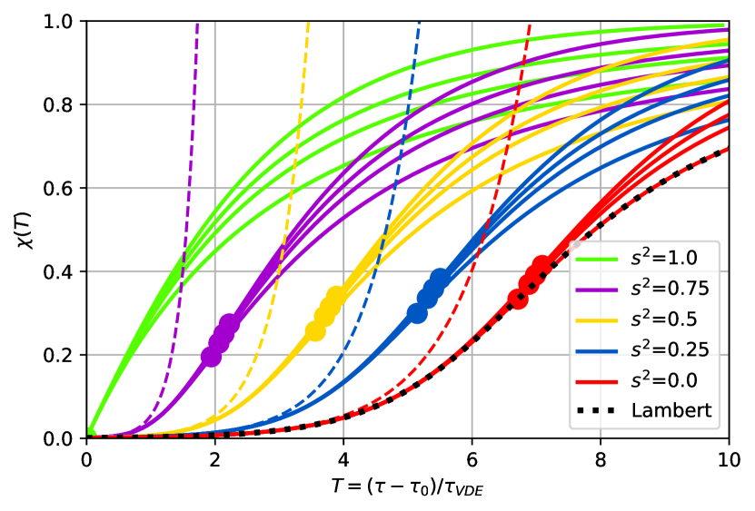
(a) slowed down by a single wall wire.

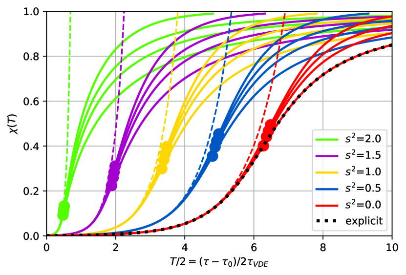
(b) slowed down by two wall wires.

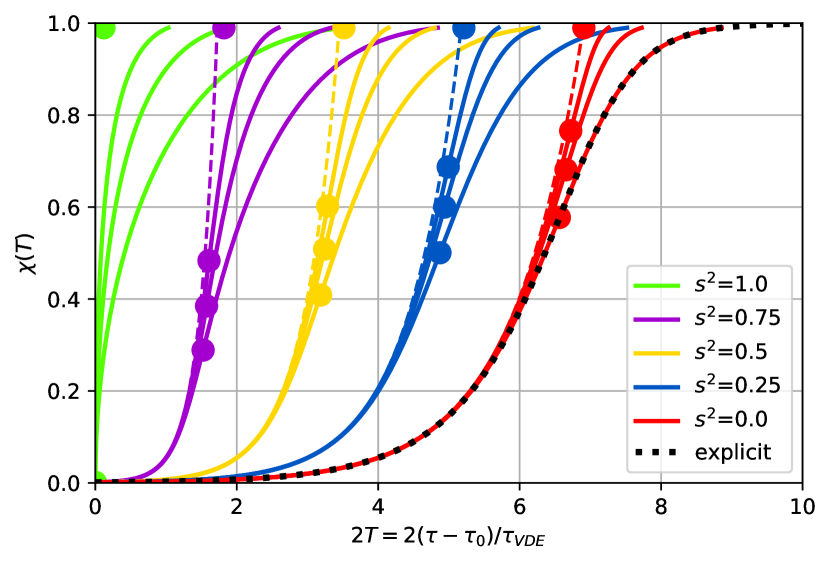
(c) surrounded by a cylindrical conducting shell.

Figure 1: Vertical drift of a plasma column due to the external field by two divertor coils (91) for varying values of $s^{2}=\gamma_{\text{VDE}}/\gamma_{\text{LR}}$ (sets of curves with different colour, see legend) and $h^{-2}\in\{0,1/3,2/3,1\}$ (bottom to top curves of same colour). The initial exponential behaviour for $T\rightarrow-\infty$ is traced by the dashed colour lines. The inflexion points, $\ddot{\bar{z}}_{*}=0$ are denoted with coloured circles. The black dotted line represents the explicit solution $\bar{z}(T,h\rightarrow\infty,s^{2}\rightarrow 0)$. For better comparison, the x-axis is adjusted so that the span is identical for the three wall models.

IV Resistive wall as a cylindrical shell

The plasma is not simply bounded by toroidal wires, it is (topologically) fully enclosed by a conducting vessel. It is thus important to study the currents that form within a thin cylindrical shell as the plasma column moves in its interior. The added dimension in 2D shells versus 1D wires allows for extra diffusion of magnetic flux in the poloidal direction, which affects the speed and behaviour of the VDE.

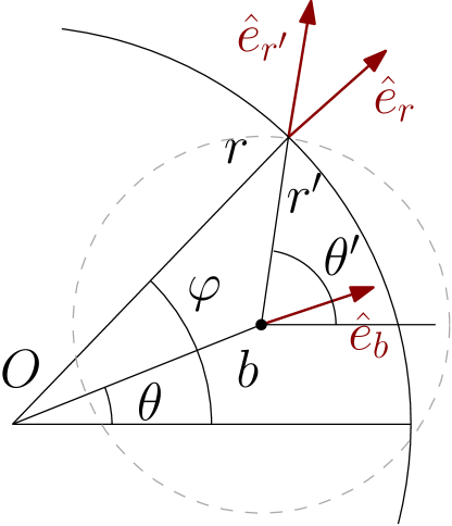
Figure 2: Choice of cylindrical coordinates and definitions of angles and radii.

In what follows, the origin of the coordinate system coincides with the axis of symmetry of the shell. The radius of the shell is the minor radius $a$ and its thickness is $\Delta$. The plasma is modelled as a straight wire floating at $x(t)=b(t)\cos[\theta(t)]$ and $y(t)=b(t)\sin[\theta(t)]$. The choice of coordinates and definition of angles and distances are sketched on figure 2.

IV.1 Fields from plasma wire and shell surface currents

First, the field produced by the plasma wire is expressed in cylindrical coordinates. As shown in the appendix D, this can be performed either by the multipole expansion of the vector potential or by solving the 2D Laplace equation given the plasma current density

$$\bm{j}_{p} =I_{p}\delta(r-b)\delta(\varphi-\theta)\bm{\nabla}r\times\bm{\nabla}\varphi$$ (54)

The resulting potential functions representing the plasma magnetic field $\bm{B}_{p}=\bm{\nabla}\Phi_{p}=\bm{\nabla}\Psi_{p}\times\bm{\nabla}z$ are

$$\Psi_{p}(r>b,\varphi) =\frac{\mu_{0}I_{p}}{2\pi}\left[-\ln\frac{r}{b}+\sum_{m=1}^{\infty}\left(\frac{b}{r}\right)^{m}\frac{\cos[m(\varphi-\theta)]}{m}\right]$$ (55)

and

$$\Phi_{p}(r>b,\varphi) =\frac{\mu_{0}I_{p}}{2\pi}\left\{\varphi+\sum_{m=1}^{\infty}\left(\frac{b}{r}\right)^{m}\frac{\sin[m(\varphi-\theta)]}{m}\right\}$$ (56)

Second, the surface current density flowing in the $z$-direction on the thin shell at $r=a$ is represented as

$$\bm{j}_{s}(r,\varphi,t)=\delta(r-a)\kappa^{\prime}(\varphi,t)\bm{\nabla}r\times\bm{\nabla}\varphi=\delta(r-a)\bm{\nabla}r\times\bm{\nabla}\kappa$$ (57)

where the surface current function $\kappa^{\prime}(\varphi,t)$ is expanded in a Fourier series as

$$\kappa^{\prime}(\varphi,t) =\sum_{m=0}^{\infty}\left[j^{s}_{m}(t)\sin(m\varphi)+j^{c}_{m}(t)\cos(m\varphi)\right]$$

$$=\frac{I_{0}(t)}{2\pi}+\sum_{m=1}^{\infty}\frac{I_{m}(t)}{\pi}\cos[m(\varphi-\alpha_{m}(t))]$$ (58)

By the same exercise as in appendix D.2, the associated potential function in the region enclosed by the shell at $r=a$ is found to be

$$\Phi_{s}(r<a,\varphi,t) =-\frac{\mu_{0}}{2\pi}\sum_{m=1}^{\infty}I_{m}\left(\frac{r}{a}\right)^{m}\frac{\sin[m(\varphi-\alpha_{m})]}{m}$$ (59)

and therefore the poloidal flux function is deduced by the Cauchy-Riemann condition (94),

$$\Psi_{s}(r<a,\varphi,t) =\frac{\mu_{0}}{2\pi}\sum_{m=1}^{\infty}I_{m}\left(\frac{r}{a}\right)^{m}\frac{\cos[m(\varphi-\alpha_{m})]}{m}.$$ (60)

One can express the magnetic field generated by surface currents on the cylindrical shell anywhere between $b<r<a$ via $\bm{B}_{s}=\bm{\nabla}\Phi_{s}=\bm{\nabla}\Psi_{s}\times\bm{\nabla}z$.

IV.2 Circuit and motion equations

If only interested in the (radial) motion of the plasma column, the phase $\alpha_{m}(t)=\theta(t)=0$ can be held fixed. The initial value of $I_{p}(0)$ is used to normalise the currents, $\bar{I}_{p}(t)=I_{p}/I_{p}(0)$ and $\bar{I}_{m}(t)=I_{m}/I_{p}(0)$.

The azimutal component of the magnetic field from the shell produces the radial force on the wire

$$M\frac{d^{2}b}{dt^{2}} =\bm{F}\cdot\bm{\nabla}r\Big{|}_{b,\theta}=lI_{p}\bm{\nabla}z\times\bm{B}_{s}\cdot\bm{\nabla}r+F_{ext}$$ (61)

$$=\frac{\mu_{0}lI_{p}}{2\pi b}\sum_{m=1}^{\infty}I_{m}\left(\frac{b}{a}\right)^{m}+F_{ext}$$ (62)

where $\cos[m(\theta-\alpha_{m})]=1$ was used, $M$ denotes here the plasma mass and $F_{ext}=I_{p}dA_{ext}/dz$ is the external force from the divertor fields. In normalised units, the equation of motion of the plasma column reads

$$\ddot{\bar{z}}=\bar{I}_{p}\left[\sum_{m=1}^{\infty}\bar{I}_{m}\bar{z}^{m-1}+\bar{A}_{\text{ext}}^{\prime}(\bar{z})\right]$$ (63)

where $\bar{z}(\tau)=b/a$, $\tau=t/t_{c}$, $t_{c}=\sqrt{Ma^{2}/L_{c}I_{p}^{2}}$, $L_{c}=\mu_{0}l/2\pi$ as before. This equation complies with (42).

In the vacuum between the shell and the plasma column, the total magnetic field produced by the plasma current $I_{p}(t)$ and surface currents $I_{m}(t)$ is

$$\bm{B}(b<r<a,\varphi,t)=\frac{\mu_{0}}{2\pi}\bm{\nabla}\Bigg{\{}I_{p}\varphi\\ +\sum_{m=1}^{\infty}\frac{\sin(m\varphi)}{m}\Bigg{[}I_{p}\left(\frac{b}{r}\right)^{m}-I_{m}\left(\frac{r}{a}\right)^{m}\Bigg{]}\Bigg{\}}$$ (64)

where the phase $\alpha_{m}(t)=0$ was omitted.

The time-variation of the total magnetic field induces an electric field (Faraday’s law), $\partial_{t}\bm{B}+\bm{\nabla}\times\bm{E}=0$, which drives current within the thin conducting shell via Ohm’s law, $\bm{E}=\eta_{w}\bm{j}$. The normal component of the magnetic field is the only useful projection since it is continuous within the shell. In the limit of an infinitesimally thin wall, it can be assumed to be radially constant across the shell. We thus have

$$\partial_{\tau}\left(\frac{\bm{B}}{B_{c}}\cdot\hat{\bm{e}}_{r}\right)_{a}=-\sum_{m=1}^{\infty}\sin(m\varphi)\frac{d}{d\tau}\left[\bar{z}^{m}\bar{I}_{p}+\bar{I}_{m}\right]$$ (65)

where $B_{c}=\mu_{0}I_{p}(0)/2\pi a$ is the initial plasma poloidal field at the shell.

The current distribution inside the thin shell is also assumed to be radially constant, with the following representation of the delta function boozer-2015

$$\delta(r-a)\overset{\Delta\rightarrow 0}{\longleftarrow}\begin{cases}\frac{1}{\Delta}&a-\Delta/2<r<a+\Delta/2\\ 0&\text{elsewhere}\end{cases}$$ (66)

so that, at $r=a$, we have

$$\hat{\bm{e}}_{r}\cdot\bm{\nabla}\times\bm{E}\big{|}_{a} =\bm{\nabla}r\cdot\bm{\nabla}\times(\eta_{w}\bm{j})\Big{|}_{a}$$

$$=-\frac{\eta_{w}}{\Delta}\bm{\nabla}\cdot[\kappa^{\prime}(\varphi,t)\bm{\nabla}r\times(\bm{\nabla}r\times\bm{\nabla}\varphi)]\Big{|}_{a}$$

$$=\frac{\eta_{w}}{\Delta}\bm{\nabla}\cdot(\kappa^{\prime}\bm{\nabla}\varphi)\Big{|}_{a}=\frac{\eta_{w}}{\Delta}\frac{\kappa^{\prime\prime}}{a^{2}}$$ (67)

where $\kappa^{\prime\prime}=\partial_{\varphi}\kappa^{\prime}$, $(\bm{\nabla}\varphi)^{2}=1/r^{2}$ and $\bm{\nabla}^{2}\varphi=0$.

Using the representation for $\kappa$ of (58) and combining (65) and (67) in Faraday’s and Ohm’s law one obtains a list of decoupled circuit equations. In normalised variables, each mode $m\geq 1$ obeys

$$\frac{d}{d\tau}\left[\frac{1}{m}\bar{I}_{m}+\bar{I}_{p}\frac{\bar{z}^{m}}{m}\right] =-2\bar{R}_{w}\bar{I}_{m}$$ (68)

where $\bar{R}_{w}^{-1}=S_{w}(\Delta/a)$, $S_{w}=\mu_{0}av_{A}/\eta_{w}$ is the wall Lundquist number and $v_{A}=a/t_{c}$ the characteristic Alfvén speed as before. This infinite list of equations is the spectral version of (44).

The last circuit equation originates from the flux change through the plasma wire. Upon evaluating $\partial_{t}\Psi_{s}|_{b,\theta}$ from (60), one arrives at

$$\frac{d}{d\tau}\left[\bar{L}_{p}\bar{I}_{p}+\sum_{i=1}^{\infty}\frac{\bar{z}^{m}}{m}\bar{I}_{m}+\bar{A}_{\text{ext}}\right]=-\bar{R}_{p}\bar{I}_{p}$$ (69)

which is analogous to (43). Notice that the shell cannot produce $m=0$ flux within its interior and therefore cannot oppose to the decay of plasma current (Gauss law).

In comparison with the model with multiple wires, the shell displays a diagonal self-inductance matrix $\mathbb{M}_{mn}=\delta_{mn}/m$ and scalar resistance $\mathbb{R}_{mn}=2\bar{R}_{w}\delta_{mn}$. The mutual inductance vector is identified as $\bar{M}_{m}=\bar{z}^{m}/m$ and we remark that

$$\vec{M}^{\prime}\cdot\vec{M}^{\prime} =\frac{1}{\bar{z}^{2}}\sum_{m=1}^{\infty}\bar{z}^{2m}=\frac{1}{1-\bar{z}^{2}}$$ (70)

$$\vec{M}^{\prime}\mathbb{M}\vec{M}^{\prime} =\frac{1}{\bar{z}^{2}}\sum_{m=1}^{\infty}\frac{\bar{z}^{2m}}{m}=-\frac{1}{\bar{z}^{2}}\ln|1-\bar{z}^{2}|$$ (71)

In the limit of a perfectly conducting shell where $\bar{R}_{w}\rightarrow 0$, the system is integrable by virtue of flux conservation. The plasma is stabilised by the presence a diverging potential, which can be shown to be $V_{\text{eff}}=-\frac{1}{2}\ln|1-\bar{z}^{2}|$.

IV.3 Resistive decay of surface currents and characteristic plasma motion

In the resistive decay regime where the slow evolution of the equilibrium position is sought for, the assumption of time-scale separation, $\ddot{\bar{z}}_{e}\ll 1$, suggests that the surface currents satisfy the spectral analogue of relation (46). Force balance requires that the mode amplitudes be the fields

$$\bar{I}_{m}(\bar{z})=-\bar{z}^{m-1}(1-\bar{z}^{2})\bar{A}_{\text{ext}}^{\prime}$$ (72)

Assuming that $\bar{I}_{p}\sim 1$ for simplicity, the motion of the equilibrium position reads from (48)

$$\dot{\bar{z}}=\frac{2\bar{R}_{w}\bar{A}_{\text{ext}}^{\prime}}{\frac{1}{1-\bar{z}^{2}}-\frac{\bar{A}_{\text{ext}}^{\prime}}{\bar{z}}\left(1+\frac{1+\bar{z}^{2}}{\bar{z}^{2}}\ln|1-\bar{z}^{2}|\right)+\bar{A}_{\text{ext}}^{\prime\prime}\frac{1-\bar{z}^{2}}{\bar{z}^{2}}\ln|1-\bar{z}^{2}|}$$ (73)

which becomes for the specific divertor field of (91)

$$\dot{\bar{z}}\left\{\frac{1-h^{-2}\bar{z}^{2}}{(1-\bar{z}^{2})\bar{z}}-s^{2}\left[\frac{1}{\bar{z}}+(1-h^{-2})\frac{2}{\bar{z}}\frac{\ln|1-\bar{z}^{2}|}{1-h^{-2}\bar{z}^{2}}\right]\right\}=2\gamma_{\text{VDE}}$$ (74)

where $\gamma_{\text{VDE}}=\bar{R}_{w}\gamma_{\text{ext}}^{2}$ as before. The implicit solution of the above ODE in the form of (21) is

$$F(\bar{z})= \frac{1}{2}\ln\left|\frac{\bar{z}^{2}}{1-\bar{z}^{2}}\right|$$ (75)

$$H(\bar{z})= \frac{1}{2}\ln\left|\frac{1}{1-\bar{z}^{2}}\right|$$ (76)

$$K(\bar{z})= \ln\bar{z}-(1-h^{-2})\left\{\text{Li}_{2}(\bar{z}^{2})+\text{Li}_{2}\left[-\frac{h^{-2}(1-\bar{z}^{2})}{1-h^{-2}}\right]\right.$$

$$\left.+\ln|1-\bar{z}^{2}|\ln\left|\frac{1-h^{-2}\bar{z}^{2}}{1-h^{-2}}\right|\right\}$$ (77)

where $\text{Li}_{2}(z)=-\int^{z}_{0}\frac{\ln(1-u)}{u}du$ is the so-called Spence function or dilogarithm. This solution is displayed on figure 1(c)) for various values of $s^{2}$ and $h$. The initial growth rate in this configuration is

$$\frac{\dot{\bar{z}}}{\bar{z}}\overset{\bar{z}\rightarrow 0}{\longrightarrow}\frac{2\gamma_{\text{VDE}}}{1-s^{2}}$$ (78)

which is twice as fast as for wire models at equal conducting cross-sections. This is an interesting difference between wire and shell models, where the extra dimension allows for diffusion of flux across the surface, additionally to in the direction of current. The time axis of figure 1(c)) is scaled so that the initial slopes match with figure 1(a)) for easier comparison.

In the limit where the divertor coils are far from the wall, $h\rightarrow\infty$, an explicit solution for $s^{2}\rightarrow 0$ is given by

$$\bar{z}(T;h\rightarrow\infty,s^{2}\rightarrow 0)=\frac{1}{\sqrt{1+e^{-4T}}}$$ (79)

This behaviour is illustrated on figure 1(c)) by the dashed black line.

In the extreme case where the divertor coils are radially located on the shell, $h\rightarrow 1$, the solution tends to preserve the asymptotic exponential behaviour

$$\bar{z}(T;h\rightarrow 1,s^{2})=e^{2T/(1-s^{2})}$$ (80)

and inflexion never occurs, as depicted by the dashed colour curve on figure 1(c)).

V Conclusion

Assuming that the plasma column behaves as a rigid rod during a VDE, a series of analytic expressions for its non-linear vertical drift across the vacuum vessel were derived. First, a basic model where the wall is treated as a single conducting wire was used to identify four timescales: the fast Alfvén, the fast oscillations around the minimum of effective potential, the slow current decay (“L over R”) time and the slower VDE rate. Well separated timescales between the Alfvén dynamics and VDE evolution was assumed based on experimental evidence. The linear analysis revealed two oscillatory modes and a slow exponentially growing mode coinciding with the vertical instability. The non-linear dynamics were shown to be solvable in the limit where the wall is a perfect conductor and the induced currents fully stabilise the plasma column by generating a strong effective potential. With weak wall resistivity, the equilibrium point relaxes towards the vessel at the rate of current dissipation. In this regime, the induced wall currents compensate the divertor field at the position of the plasma column. The force balance condition was used to eliminate the fast oscillatory motion and capture the non-linear relaxation process into a single ODE.

The model was extended to an arbitrary number of wall wires via a Lagrangian principle, where the decay of currents is incorporated through the Rayleigh dissipation function. A general ODE for the vertical drift of the plasma, equation (48), was derived in the limit of weak resistivity. The case where the plasma is surrounded by two wall wires was studied analytically. Although the initial growth rate is almost identical for equivalent combined cross-sections, the characteristic motion with two wall wires was shown to be steeper and the inflexion point farther than in the case with only a single wall wire.

The methodology was finally applied to the case where the wall is represented as a thin cylindrical shell. The vector potential produced by surface currents on the wall was expressed in cylindrical coordinates via the standard solution to the two-dimensional Laplace equation. An infinite system of circuit equations was then obtained for the Fourier modes of the surface current and the corresponding resistance and inductance matrices of the shell were identified. Inserted into the single ODE (48), the infinite series produced logarithmic functions for the VDE dynamics and an analytic solution was obtained.

A study of more general geometries for the surrounding conducting structures can be performed analytically or numerically in a straightforward, robust and efficient way by computing the wall inductance and resistance matrices as well as the plasma-wall mutual-inductance vector with the identities reported in appendix A.

In all systems studied, it was found that the motion deviates from the exponential growth expected from linear analysis and becomes a more complex algebraic deceleration. It was observed that the instantaneous growth rate, $\dot{\bar{z}}/\bar{z}$, monotonically decreases to zero as the plasma reaches the wall, while the acceleration $\ddot{\bar{z}}$ crosses zero at the inflexion point. For a given divertor height, the inflexion point is closer to the wall when the external field is weaker. The maximum inflexion point is a purely geometric quantity that can be used experimentally as a reference point to locate a change of physics. Indeed, experimental reconstruction of the magnetic axis position often show that the plasma column accelerates towards the wall near the end of a VDE. The fact that our model contradicts this observation leads us to conclude that, if no inflexion occurs, the physics controlling the VDE evolution is non-inductive. If the magnetic axis is found to accelerate, for example as in the NSTX gerhardt-2012 , the VDE is most probably driven by the sharing of current between the edge plasma and the wall, the scraping of the last-closed flux surfaces and/or from the internal thermal quench dynamics. If the plasma slows down in the vicinity of the wall, as seen in JET upward VDEs gerasimov-2015 , the inductive component is dominant. In the latter case, the picture of a slowly evolving three-dimensional equilibrium zakharov-2008 seems a suitable model, while in the former more physics (MHD and beyond) must be invoked.

References

Appendix A Circuit equations, inductance and resistance matrices from variational principle

The Lagrangian (41), which leads to the motion and circuit equations (42-44), essentially consists of the plasma kinetic energy and the total magnetic energy produced by the plasma, wall and external coils. The framework is valid for 2D and 3D conducting structures, beyond the application to discrete set of wires and filaments. In fact, the equations for the plasma surrounded by a cylindrical shell (63, 68 and 69) could have been derived using the Lagrangian principle directly. Indeed, recalling that $\bm{\nabla}\cdot(\bm{A}\times\bm{B})=(\bm{\nabla}\times\bm{A})\cdot\bm{B}-\bm{A}\cdot(\bm{\nabla}\times\bm{B})$ and assuming that the magnetic field vanishes at infinity, the total magnetic energy can be expressed as

$$\mathcal{L}_{M} =\frac{1}{2\mu_{0}}\int_{\mathbb{R}^{3}}B^{2}d\omega=\frac{1}{2}\int_{\Omega}\bm{A}\cdot\bm{j}d\omega$$ (81)

where $\Omega$ is the support of the current density $\bm{j}=\bm{\nabla}\times\bm{B}/\mu_{0}$. Decomposing the total magnetic field into the plasma, wall and external components $\bm{B}=\bm{B}_{p}+\bm{B}_{w}+\bm{B}_{ext}$, the wall inductance matrix is obtained as

$$N\mathbb{M}_{mn}=\frac{1}{2}\frac{\partial^{2}}{\partial\bar{I}_{m}\partial\bar{I}_{n}}\int_{\text{wall}}\bm{A}_{w}\cdot\bm{j}_{w}d\omega$$ (82)

where $\bar{I}_{m}$ are adimensional degrees of freedom chosen to represent wall currents and $N=L_{c}I_{p}(0)^{2}$ the normalisation factor. The plasma-wall mutual inductance vector is

$$N\vec{M}=\frac{\partial^{2}}{\partial\vec{I}\partial\bar{I}_{p}}\int_{\text{wall}}\bm{A}_{p}\cdot\bm{j}_{w}d\omega=\frac{\partial^{2}}{\partial\vec{I}\partial\bar{I}_{p}}\int_{\text{plasma}}\bm{A}_{w}\cdot\bm{j}_{p}d\omega$$ (83)

where $\bar{I}_{p}=I_{p}/I_{p}(0)$ is the normalised plasma current. Notice the reciprocity of the latter expression. Similarly, the external potential generated by the divertor coils can be expressed as

$$L_{c}I_{p}(0)\bar{A}_{\text{ext}}=\frac{\partial}{\partial\bar{I}_{p}}\int_{\text{plasma}}\bm{A}_{ext}\cdot\bm{j}_{p}d\omega.$$ (84)

The Rayleigh dissipation function essentially conveys the Ohmic power loss

$$\mathcal{D}=\frac{1}{2}\int_{\Omega}\eta\bm{j}^{2}d\omega$$ (85)

so that the resistance matrix may be expressed as

$$\frac{v_{A}N}{a}\mathbb{R}_{mn}=\frac{1}{2}\frac{\partial^{2}}{\partial\bar{I}_{m}\partial\bar{I}_{n}}\int_{\text{wall}}\eta_{w}\bm{j}^{2}_{w}d\omega$$ (86)

where care must be taken with squared delta-functions from the filament or surface current density.

The reader may verify that the diagonal inductance and resistance matrices for the cylindrical shell presented in section (IV) are correctly recovered through these identities. They are particularly useful in the context of a spectral or Finite Element representation of wall currents. It is mentioned that the motion of the plasma column within a toroidally shaped wall can be studied in this way too.

Appendix B Coil inductances

Self-inductance and mutual inductance of filaments are purely geometric coefficients that can be acquired experimentally or estimated analytically. The expression and interpretation of self-inductance via Neumann formula is somewhat subtle because it formally diverges (rosa, ). The normalised self-inductance of a thin circular coil of perimeter $l=2\pi R$ is given for a uniform current density by essen-2013

$$\bar{L}=\frac{L}{L_{c}}=-\left[\ln\left(\frac{\epsilon\delta}{8}\right)+\frac{7}{4}\right]$$ (87)

where $\delta=\Delta/a$ is the normalised diameter of the coils, $\epsilon=a/R$ the inverse aspect ratio and $L_{c}=\mu_{0}l/2\pi=\mu_{0}R$.

The normalised mutual inductance, $\bar{M}(\bar{z})=M(z)/L_{c}$ where $L_{c}=\mu_{0}l/2\pi$, of two circular coils of equal major radius $R=a/\epsilon$ is given as a function of the separating normalised vertical distance $\bar{z}=z/a$ by essen-2009

$$\bar{M}(\bar{z})=\frac{1}{k}\left[(2-k^{2})K(k^{2})-2E(k^{2})\right]$$ (88)

where $K(m)=\int_{0}^{\pi/2}\frac{d\theta}{\sqrt{1-m\sin^{2}\theta}}$ is the complete elliptic integral of the first kind, $E(m)=\int_{0}^{\pi/2}\sqrt{1-m\sin^{2}\theta}d\theta$ the complete elliptic integral of second kind,

$$k(\bar{z})=\frac{1}{\sqrt{1+(\frac{\epsilon\bar{z}}{2})^{2}}}$$ (89)

and $\epsilon=a/R$ is the inverse aspect ratio.

It is noted that the argument of the elliptic functions is bounded by $2/\sqrt{5}\cong 0.89\leq k\leq 1$. Due to the logarithmic divergence of $K(k)$ as $k\rightarrow 1$, the mutual inductance of two circular coils becomes well approximated by

$$\bar{M}(\bar{z})\longrightarrow-\ln(\epsilon\bar{z})$$ (90)

corresponding to the mutual inductance of two straight wires. Toroidicity is seen to play a minor role in the derivative of the mutual inductance representing the Lorentz force between two wires, $\bar{M}^{\prime}\rightarrow-1/\bar{z}$.

Appendix C External potential from divertor coils

Vertical Displacement Events (VDEs) are driven by the external potential produced by the two divertor coils giving the plasma its elongation. We assume for simplicity that the currents in each divertor coil are fixed and identical $\bar{I}_{c}=I_{c}/I_{p}(0)$ and that the coils are positioned symmetrically about the origin, at $z=z_{c}>a$ and $z=-z_{c}<-a$. The (normalised) external force is given by (see appendix B)

$$\bar{F}_{\text{ext}} =\bar{I}_{c}[\bar{M}^{\prime}(\bar{z}-h)+\bar{M}^{\prime}(\bar{z}+h)]$$ (91)

$$=\bar{I}_{c}\left(\frac{1}{h-\bar{z}}-\frac{1}{h+\bar{z}}\right)=\frac{\gamma_{\text{ext}}^{2}\bar{z}}{1-h^{-2}\bar{z}^{2}}$$ (92)

where $\bar{z}=z/a$, $h=z_{c}/a$ and $\gamma_{\text{ext}}^{2}\equiv 2\bar{I}_{c}/h^{2}$ is the inverse width of the quadratic potential at the unstable equilibrium point. In toroidal shaped plasmas, one can invoke radial force balance and $\bm{\nabla}\times\bm{B}_{ext}=0$ in order to relate the $\gamma_{\text{ext}}$ parameter to the so-called field decay index $n$ (parametrisation of the vertical field as $B_{Z}\propto R^{-n}$) and the plasma inductance $\bar{L}_{p}=L_{p}/L_{c}$ lazarus-1990 ; shafranov-1963

$$\gamma_{\text{ext}}^{2}\sim\epsilon^{2}\bar{L}_{p}n$$ (93)

where $\epsilon=a/R$ is the inverse aspect ratio.

Appendix D Field from the plasma wire on the cylindrical shell

In the vacuum region, the poloidal magnetic field produced by the plasma wire satisfies two conditions. First, $\bm{\nabla}\cdot\bm{B}_{p}=0$, true for any magnetic field, implies that $\bm{B}_{p}=\bm{\nabla}\times\bm{A}_{p}$. By symmetry along the cylinder’s axis $z$, the vector potential is represented by the poloidal flux function only as $\bm{A}_{p}=\Psi_{p}\bm{\nabla}z$ or $\bm{B}_{p}=\bm{\nabla}\Psi_{p}\times\bm{\nabla}z$. Secondly, $\bm{\nabla}\times\bm{B}_{p}=0$ since there are no currents in the vacuum region, which implies that the poloidal field is also represented by the gradient of a potential function $\Phi_{p}$, $\bm{B}_{p}=\bm{\nabla}\Phi_{p}$. By combining those conditions, one concludes that both potentials function are harmonic, $\bm{\nabla}^{2}\Phi_{p}=0$ and $\bm{\nabla}^{2}\Psi_{p}=0$. They in fact form what is called a pair of harmonic conjugate functions which satisfies $\bm{\nabla}\Phi_{p}\cdot\bm{\nabla}\Psi_{p}=0$ and Cauchy-Riemann equations

$$r\partial_{r}\Phi_{p} =\partial_{\varphi}\Psi_{p} \partial_{\varphi}\Phi_{p} =-r\partial_{r}\Psi_{p}.$$ (94)

There are two ways to evaluate $\Psi_{p}$ and $\Phi_{p}$ in the natural coordinates of the cylindrical shell. It is instructive to detail both of them.

D.1 Multipole expansion of the vector potential

The magnetic field produced by a straight wire traversed by current $I_{p}$ is easy to express as a function of the separating distance $r^{\prime}$ as in figure 2

$$\bm{B}_{p}(r^{\prime},\theta^{\prime})=\frac{\mu_{0}I_{p}}{2\pi r^{\prime}}\hat{\bm{e}}_{\theta^{\prime}}$$ (95)

where $\hat{\bm{e}}_{\theta^{\prime}}=\hat{\bm{e}}_{z}\times\hat{\bm{e}}_{r^{\prime}}=\bm{\nabla}z\times\bm{\nabla}r^{\prime}$. The corresponding poloidal flux is then written as

$$\Psi_{p}(r^{\prime},\theta^{\prime})=-\frac{\mu_{0}I_{p}}{2\pi}\ln r^{\prime}$$

For the purpose of calculating the effect of this field on a cylindrical conducting shell, a change of coordinates is performed

$$r\hat{\bm{e}}_{r} =r^{\prime}\hat{\bm{e}}_{r^{\prime}}+b\hat{\bm{e}}_{b} r^{\prime} =\sqrt{r^{2}+b^{2}-2br\hat{\bm{e}}_{b}\cdot\hat{\bm{e}}_{r}}$$

where $\hat{\bm{e}}_{b}\cdot\hat{\bm{e}}_{r}=\cos(\varphi-\theta)$. The poloidal flux then reads

$$\Psi_{p}(r,\varphi)=-\frac{\mu_{0}I_{p}}{4\pi}\ln\left[r^{2}+b^{2}-2br\cos(\varphi-\theta)\right].$$ (96)

Noting that

$$\ln|1-2\epsilon\cos\alpha+\epsilon^{2}| =\ln|1-\epsilon e^{i\alpha}|+\ln|1-\epsilon e^{-i\alpha}|$$

$$=\sum_{m=1}^{\infty}(-1)^{m+1}(-1)^{m}\frac{\epsilon^{m}}{m}\left(e^{im\alpha}+e^{-im\alpha}\right)$$

$$=\sum_{m=1}^{\infty}\frac{-2\epsilon^{m}}{m}\cos(m\alpha)$$ (97)

for $\epsilon<1$, the poloidal flux can be written as a multipole expansion

$$\Psi_{p}(r>b,\varphi) =\frac{\mu_{0}I_{p}}{2\pi}\left[-\ln r+\sum_{m=1}^{\infty}\left(\frac{b}{r}\right)^{m}\frac{\cos[m(\varphi-\theta)]}{m}\right]$$ (98)

$$\Psi_{p}(r<b,\varphi) =\frac{\mu_{0}I_{p}}{2\pi}\left[-\ln b+\sum_{m=1}^{\infty}\left(\frac{r}{b}\right)^{m}\frac{\cos[m(\varphi-\theta)]}{m}\right]$$ (99)

The associated potential function is then shown via (94) to be

$$\Phi_{p}(r>b,\varphi) =\frac{\mu_{0}I_{p}}{2\pi}\left\{\varphi+\sum_{m=1}^{\infty}\left(\frac{b}{r}\right)^{m}\frac{\sin[m(\varphi-\theta)]}{m}\right\}$$ (100)

$$\Phi_{p}(r<b,\varphi) =-\frac{\mu_{0}I_{p}}{2\pi}\sum_{m=1}^{\infty}\left(\frac{r}{b}\right)^{m}\frac{\sin[m(\varphi-\theta)]}{m}$$ (101)

D.2 Solution to 2D Laplace from wire current distribution

The current distribution from the wire is represented as ($\hat{e}_{\varphi}=r\bm{\nabla}\varphi$)

$$\bm{j}_{p} =I_{p}\delta(\bm{x}-\bm{x}_{p})\bm{e}_{z}=\frac{I_{p}}{r}\delta(r-b)\delta(\varphi-\theta)\hat{\bm{e}}_{r}\times\hat{\bm{e}}_{\varphi}$$

$$=I_{p}\delta(r-b)\delta(\varphi-\theta)\bm{\nabla}r\times\bm{\nabla}\varphi$$ (102)

The dirac delta in angles can be represented by an infinite Fourier series as

$$\delta(\varphi-\theta)\equiv\frac{1}{2\pi}+\frac{1}{\pi}\sum_{m=1}^{\infty}\cos[m(\varphi-\theta)]$$ (103)

so that

$$\mu_{0}\bm{j}_{p}=\bm{\nabla}\times\left\{-\frac{\mu_{0}I_{p}}{2\pi}\delta(r-b)\left[\varphi+2\sum_{m=1}^{\infty}\frac{\sin[m(\varphi-\theta)]}{m}\right]\bm{\nabla}r\right\}$$ (104)

Since $\mu_{0}\bm{j}_{p}=\bm{\nabla}\times\bm{B}_{p}$, it is then natural to write the magnetic field as

$$\bm{B}_{p}=-\frac{\mu_{0}I_{p}}{2\pi}\delta(r-b)\left[\varphi+2\sum_{m=1}^{\infty}\frac{\sin[m(\varphi-\theta)]}{m}\right]\bm{\nabla}r+\bm{\nabla}\Phi_{p}$$ (105)

where the potential function must satisfy $\bm{\nabla}\cdot\bm{B}_{p}=\bm{\nabla}^{2}\Phi_{p}=0$ everywhere in the vacuum. The solution $\Phi_{p}^{\pm}=\bar{\Phi}_{p}^{\pm}+\tilde{\Phi}_{p}^{\pm}$ is broken in the region enclosed by the singular layer at $r=b$ (the minus solution) and outside (the plus solution) into a component $\tilde{\Phi}_{p}$ that is single-valued in $\varphi$ and a secular term $\bar{\Phi}_{p}\propto\varphi$. The latter provides the current within the radius $r$ through the circulation $\oint\bm{B}_{p}\cdot d\bm{l}/2\pi=\int\mu_{0}\bm{j}_{p}\cdot d\bm{\sigma}/2\pi$. Hence,

$$\bar{\Phi}_{p}(r,\varphi)=\frac{\mu_{0}I_{p}}{2\pi}\varphi\Theta(r-b)$$ (106)

where $\Theta(x)$ is the Heavyside distribution, $\Theta^{\prime}=\delta$.

In the enclosed region, the single-valued solution to the 2D Laplace equation $\tilde{\Phi}_{p}^{-}$ will have to be of the following form to avoid singularities at $r=0$

$$\tilde{\Phi}_{p}(r<b,\varphi)=A^{-}\\ +\sum_{m=1}^{\infty}\left(\frac{r}{b}\right)^{m}\left(S^{-}_{m}\sin[m(\varphi-\theta)]+C^{-}_{m}\cos[m(\varphi-\theta)]\right)$$ (107)

and in the outer region to avoid diverging magnetic fields as $r\rightarrow\infty$, the single-valued solution must be of the form

$$\tilde{\Phi}_{p}(r>b,\varphi)=A^{+}+B^{+}\ln r\\ +\sum_{m=1}^{\infty}\left(\frac{b}{r}\right)^{m}\left(S^{+}_{m}\sin[m(\varphi-\theta)]+C^{+}_{m}\cos[m(\varphi-\theta)]\right)$$ (108)

The constant coefficients $A^{+}$ and $A^{-}$ play no role and can be omitted.

By virtue of $\bm{\nabla}\cdot\bm{B}_{p}=0$, the normal component of the magnetic field $\bm{B}_{p}\cdot\hat{\bm{e}}_{r}=\partial_{r}\Phi_{p}$ is continuous across the singular layer at $r=b$, which provides the matching conditions

$$B^{+} =0 S_{m}^{+} =-S_{m}^{-} C_{m}^{+} =-C_{m}^{-}$$ (109)

By integrating the continuous normal component of the magnetic field (105) across the singular layer, another matching condition is obtained as

$$\int_{b-\epsilon}^{b+\epsilon}dr\bm{B}_{p}\cdot\hat{\bm{e}}_{r}=-\frac{\mu_{0}I_{p}}{2\pi}\left[\varphi+2\sum_{m=1}^{\infty}\frac{\sin[m(\varphi-\theta)]}{m}\right]\\ +\Phi_{p}(b+\epsilon,\varphi)-\Phi_{p}(b-\epsilon,\varphi)\overset{\epsilon\rightarrow 0}{\longrightarrow}0$$ (110)

which means that

$$C_{m}^{+} =C_{m}^{-}=0 S_{m}^{+}=-S_{m}^{-}=\frac{\mu_{0}I_{p}}{2\pi m}$$ (111)

and one obtains exactly the same solution as (100-101). Notice how the representations of the magnetic field (95) and (105) are exactly the same.

References

- (1) E. Lazarus, J. Lister, and G. Neilson, Nuclear Fusion 30, 111 (1990).
- (2) M. A. Pick, P. Noll, P. Barabaschi, F. B. Marcus, and L. Rossi, Evidence of halo currents in JET, in [Proceedings] The 14th IEEE/NPSS Symposium Fusion Engineering, pp. 187–190 vol.1, 1991.
- (3) V. Riccardo, P. Andrew, A. Kaye, and P. Noll, Fusion Science and Technology 43, 493 (2003).
- (4) Y. Neyatani, R. Yoshino, and T. Ando, Fusion Technology 28, 1634 (1995).
- (5) S. Gerhardt, J. Menard, S. Sabbagh, and F. Scotti, Nuclear Fusion 52, 063005 (2012).
- (6) T. Hender, J. Wesley, J. Bialek, A. Bondeson, A. Boozer, R. Buttery, A. Garofalo, T. Goodman, R. Granetz, Y. Gribov, O. Gruber, M. Gryaznevich, G. Giruzzi, S. Günter, N. Hayashi, P. Helander, C. Hegna, D. Howell, D. Humphreys, G. Huysmans, A. Hyatt, A. Isayama, S. Jardin, Y. Kawano, A. Kellman, C. Kessel, H. Koslowski, R. L. Haye, E. Lazzaro, Y. Liu, V. Lukash, J. Manickam, S. Medvedev, V. Mertens, S. Mirnov, Y. Nakamura, G. Navratil, M. Okabayashi, T. Ozeki, R. Paccagnella, G. Pautasso, F. Porcelli, V. Pustovitov, V. Riccardo, M. Sato, O. Sauter, M. Schaffer, M. Shimada, P. Sonato, E. Strait, M. Sugihara, M. Takechi, A. Turnbull, E. Westerhof, D. Whyte, R. Yoshino, H. Zohm, D. the ITPA MHD, and M. C. T. Group, Nuclear Fusion 47, S128 (2007).
- (7) M. Lehnen, K. Aleynikova, P. Aleynikov, D. Campbell, P. Drewelow, N. Eidietis, Y. Gasparyan, R. Granetz, Y. Gribov, N. Hartmann, E. Hollmann, V. Izzo, S. Jachmich, S.-H. Kim, M. Kočan, H. Koslowski, D. Kovalenko, U. Kruezi, A. Loarte, S. Maruyama, G. Matthews, P. Parks, G. Pautasso, R. Pitts, C. Reux, V. Riccardo, R. Roccella, J. Snipes, A. Thornton, and P. de Vries, Journal of Nuclear Materials 463, 39 (2015).
- (8) J. P. Freidberg, Plasma Physics and Fusion Energy, Cambridge University Press, 2007.
- (9) S. Jardin and D. Larrabee, Nuclear Fusion 22, 1095 (1982).
- (10) S. Jardin, N. Pomphrey, and J. Delucia, Journal of Computational Physics 66, 481 (1986).
- (11) R. Sayer, Y.-K. Peng, S. Jardin, A. Kellman, and J. Wesley, Nuclear Fusion 33, 969 (1993).
- (12) Y. Q. Liu, A. Bondeson, C. M. Fransson, B. Lennartson, and C. Breitholtz, Physics of Plasmas 7, 3681 (2000).
- (13) E. Strumberger, P. Merkel, M. Sempf, and S. Günter, Physics of Plasmas 15, 056110 (2008).
- (14) S. Galkin, A. Ivanov, S. Medvedev, and Y. Poshekhonov, Nuclear Fusion 37, 1455 (1997).
- (15) F. Villone, G. Ramogida, and G. Rubinacci, Fusion Engineering and Design 93, 57 (2015).
- (16) R. Khayrutdinov and V. Lukash, Journal of Computational Physics 109, 193 (1993).
- (17) F. Villone, G. Ramogida, and G. Rubinacci, Fusion Engineering and Design 93, 57 (2015).
- (18) N. Ferraro and S. Jardin, Journal of Computational Physics 228, 7742 (2009).
- (19) C. Sovinec, A. Glasser, T. Gianakon, D. Barnes, R. Nebel, S. Kruger, S. Plimpton, A. Tarditi, M. Chu, and the NIMROD Team, J. Comp. Phys. 195, 355 (2004).
- (20) G. Huysmans and O. Czarny, Nuclear Fusion 47, 659 (2007).
- (21) D. Pfefferlé, N. Ferraro, S. Jardin, I. Krebs, and A. Bhattacharjee, Physics of Plasmas accepted (2018).
- (22) L. E. Zakharov, Physics of Plasmas 15, 062507 (2008).
- (23) S. Gerasimov, P. Abreu, M. Baruzzo, V. Drozdov, A. Dvornova, J. Havlicek, T. Hender, O. Hronova, U. Kruezi, X. Li, T. Markovič, R. Pánek, G. Rubinacci, M. Tsalas, S. Ventre, F. Villone, L. Zakharov, and J. Contributors, Nuclear Fusion 55, 113006 (2015).
- (24) V. Mukhovatov and V. Shafranov, Nuclear Fusion 11, 605 (1971).
- (25) G. Ambrosino and R. Albanese, IEEE Control Systems 25, 76 (2005).
- (26) V. Pustovitov, Nuclear Fusion 55, 113032 (2015).
- (27) A. Y. Aydemir, Joint Varenna-Lausanne International Workshop on Theory of Fusion Plasmas (2000).
- (28) H. Essén, European Journal of Physics 30, 515 (2009).
- (29) J. Bialek, A. H. Boozer, M. E. Mauel, and G. A. Navratil, Physics of Plasmas 8, 2170 (2001).
- (30) D. I. Kiramov and B. N. Breizman, Physics of Plasmas 24, 100702 (2017).
- (31) A. H. Boozer, Nuclear Fusion 55, 025001 (2015).
- (32) E. Rosa, The self and mutual inductances of linear conductors, Bureau of Standards, 1908.
- (33) H. Essen, J. C.-E. Sten, and A. B. Nordmark, Progress In Electromagnetics Research B 46, 357 (2013).
- (34) V. D. Shafranov, Journal of Nuclear Energy. Part C, Plasma Physics, Accelerators, Thermonuclear Research 5, 251 (1963).