A Model of the Cosmic Infrared Background Produced by Distant Galaxies

Abstract

The extragalactic background radiation produced by distant galaxies emitting in the far infrared limits the sensitivity of telescopes operating in this range due to confusion. We have constructed a model of the infrared background based on numerical simulations of the large-scale structure of the Universe and the evolution of dark matter halos. The predictions of this model agree well with the existing data on source counts. We have constructed maps of a sky field with an area of 1 deg² directly from our simulated observations and measured the confusion limit. At wavelengths $100-300$ $\mu$m the confusion limit for a 10-m telescope has been shown to be at least an order of magnitude lower than that for a 3.5-m one. A spectral analysis of the simulated infrared background maps clearly reveals the large-scale structure of the Universe. The two-dimensional power spectrum of these maps has turned out to be close to that measured by space observatories in the infrared. However, the fluctuations in the number of intensity peaks observed in the simulated field show no clear correlation with superclusters of galaxies; the large-scale structure has virtually no effect on the confusion limit.

1 Introduction

The sky background consists of many components that can be divided into two groups. The first group includes all of the components associated with our Galaxy and the Solar system, such as the zodiacal light and the Galactic “cirrus”. The second group is not associated with our Galaxy. The spectrum of this component has two peaks. The first peak produced by the cosmic microwave background (CMB) is in the millimeter wavelength range, while the second one is in the far infrared (IR). The latter is called the cosmic IR background (CIB). The CIB in the wavelength range 100–600 $\mu$m is believed to be due mainly to the emission of galaxies at redshifts $z\sim 1-2$ with active star formation and a large amount of dust that reradiates much of the starlight in the far IR with an intensity maximum near 100 $\mu$m (in the rest frame).

At an angular resolution that the single telescopes designed for far-IR observations usually have, the CIB is not resolved completely into individual sources and consists of spots with different brightnesses. The spatial CIB fluctuations create the so-called confusion problem, where the faint point sources cannot be separated from the spots produced by many distant galaxies. This effect limits the sensitivity of photometric studies in the far-IR and submillimeter ranges.

Future far-IR observatories, such as Millimetron (http://millimetron.ru, Wild et al. (2009); Smirnov et al. (2012); Kardashev et al. (2014)), CALLISTO, and OST, will be able to distinguish much more details on IR sky maps than are accessible in the currently available observations. Therefore, to predict the influence of confusion for future observations, it is necessary to construct a model capable of extrapolating the current views of the CIB to a higher resolution and sensitivity.

The goal of this paper is to construct a CIB model to predict the possibilities of observations with the Millimetron space telescope and other similar space observatories. It should be emphasized that this CIB model is based on the halo catalog produced with one of the advanced numerical models for the evolution of the matter distribution in the Universe. This allows us to study in detail the manifestations of the large-scale structure of the Universe on the CIB maps. Since a large number of CIB models and approaches to their construction exist at present, it turns out to be important to classify these models and approaches as well as to choose the most suitable ones for our purposes from them.

2 Classification of CIB models

o construct a CIB model, it is necessary to specify the spatial distribution of galaxies and their spectra. The existing approaches to modeling the CIB can be divides into three groups: backward evolution, forward evolution, and a semi-analytical method. The first two approaches (methods) are described in the review by Lonsdale (1996). Let us briefly consider the approaches listed above.

The method of backward evolution is based on the assumption that the evolution of model parameters known from observations of the local Universe and observations at some redshifts can be specified in the direction of increasing redshift, i.e., in the direction opposite to the natural evolution (from the formation of objects to the present day). Many papers are de- voted to modeling by this method (see, e.g. Franceschini et al. (2010); Rowan-Robinson (2009); Valiante et al. (2009); Lagache et al. (2003); Dole et al. (2003); Béthermin et al. (2011)). Usually, a known luminosity function is taken in the method of backward evolution and its parameters are assumed to evolve with redshift z. The free model parameters determine precisely how they evolve. A library of spectra is used to describe several galaxy populations. Depending on model complexity, the shapes of the spectra may or may not depend on z or luminosity. For example, there can be two (Béthermin et al., 2011; Béthermin et al., 2012; Dole et al., 2003), four (Jeong et al., 2006; Rowan-Robinson, 2009) or five (Franceschini et al., 2010; Gruppioni et al., 2011) galaxy populations. In some papers, instead of approximating the evolution of the luminosity function, it is calculated from the evolution of the star formation rate (Béthermin et al., 2012) or from the assumption that the stellar mass function evolves with star formation and other processes are taken into account (Weinmann et al., 2012). It is possible to use the color–luminosity function rather than the luminosity function (Rahmati & van der Werf, 2011).

Different approaches are also possible in the methods of determining the free parameters. For example, all of the available source counts and/or luminosity functions (Béthermin et al., 2011; Franceschini et al., 2010; Gruppioni et al., 2011; Rahmati & van der Werf, 2011; Rowan-Robinson, 2009; Valiante et al., 2009), CIB spectra (Franceschini et al., 2010), redshift distributions of objects with fluxes above a certain one for different wavelengths (Franceschini et al., 2010; Rahmati & van der Werf, 2011) can be used, or the parameters are specified from model assumptions (Béthermin et al., 2012; Dole et al., 2003).

The effects of strong gravitational lensing of sources at high redshifts should also be taken into account. The need for this is confirmed by the detection of bright lensed objects at high redshifts in the (sub)millimeter range (Vieira et al., 2013; Negrello et al., 2010). Both a magnification of the source and a change in its angular size must be observed in the case of strong gravitational lensing. Its multiple images can also be observed in the case of a sufficient telescope resolution. Since the submillimeter telescopes have a limited spatial resolution and, consequently, are subjected to confusion, the lensed unresolved distant sources must contribute significantly to the background radiation at submillimeter wavelengths. The expected number of lensed sources at 500 $\mu$m with a flux of more than 100 mJy is about 15%, and this fraction increases to 40% at about 1 mm (Béthermin et al., 2011).

It should be noted that the method of backward evolution is not based on any physical model; it is based largely on observational data fitting. If we choose the shape of the luminosity function, choose the spectra, and carefully specify or fit the free parameters, then any observational data can be fitted in principle. Thus, this method has a good descriptive power but a very poor predictive one. At a small amount of observational data its application can lead to results far from reality (see, e.g., Domínguez et al. (2011)).

It is important to note that only the source counts as a function of the flux, redshift, and luminosity are obtained at the “output” of the method of backward evolution. This approach gives no information about the spatial distribution of sources and the association of galaxies with the distribution of dark matter.

The method of forward evolution is also described in detail in many papers (see, e.g., Lonsdale (1996); Devriendt & Guiderdoni (2000); Bouché et al. (2010)). Its basic idea is the construction of a semi-analytical model for the evolution of dark matter halos in accordance, for example, with the Press–Schechter formalism. The halo mass function and its evolution with redshift are calculated from this model. Thereafter, the mass function is converted to the luminosity functions of one or more types of galaxies by taking into account their evolution (Conroy & Wechsler, 2009; Hopkins et al., 2008), the star formation processes, the evolution of stars, the feedback, dust absorption and emission effects (Guiderdoni et al., 1998; Devriendt & Guiderdoni, 2000; Bouché et al., 2010; Granato et al., 2004; Lacey et al., 2010; Cole et al., 2000), the accretion onto black hole (Granato et al., 2004; Hopkins et al., 2008), etc.

A major shortcoming of the classical approach of forward evolution is that the results obtained characterize the background only on average. This method, along with the method of backward evolution, makes it possible to determine the number of sources in a specified range of wavelengths and fluxes but not properties (coordinates, luminosities, spectra) of individual sources.

The third approach, called semi-analytical, was used in a number of papers to determine the properties of galaxies in the optical and near-IR ranges (see, e.g., Cattaneo et al. (2005, 2006); Cousin et al. (2015)). This approach uses a numerical model for the evolution of dark matter based on which a halo catalog is produced. Baryonic matter is then added to each halo. Various processes, such as the accretion of gas from the parent halo, the star formation, the activity in galactic nuclei, the feedback, the gas outflow, the formation of a disk, a bulge, etc., are taken into account in this case. The specific ways of allowance for these processes are highly varied. In contrast to the method of forward evolution, in the semi-analytical method numerical models are used instead of the evolution of the mass functions to obtain information about the evolution of dark matter halos.

Various approaches, for example, the iterative technique, as in Henriques et al. (2013), can be used to specify the free parameters of semi-analytical models just as in other methods. In recent years the semi-analytical methods based on numerical simulations of the dark matter distribution have gained a major development. In particular, they allow one to trace a detailed picture of galaxy evolution and, as a consequence, to obtain the mass functions of various components, the stellar mass-halo mass relationship at various $z$, the luminosity functions, the color–magnitude diagrams, the Tully–Fisher relations, the color–mass diagram, the evolution of the star formation rate with redshift, the distribution of star formation rates in galaxies at various z, the dependence of the stellar mass of the bulge on the total mass of the bulge, the evolution of the star density $\rho_{*}$[̇$M_{\odot}$Mpc^-1] with $z$, the correlation between the masses of black holes and bulges, the luminosity function of quasars, the evolution of the fraction of active galactic nuclei (AGNs), and the evolution of the black hole mass function.

It should be noted that the approach used here can be attributed to this type, i.e., to the semi-analytical approach.

3 Model description

3.1 Model requirements

The goal of model construction is to determine the possibilities of observing objects with low fluxes (faint objects) and to investigate the large-scale structure of the Universe with space observatories operating in the far IR and having an aperture of about 10 m. The following parameters of the Millimetron observatory (Smirnov et al., 2012) were taken as a basis:

1. The angular resolution of the telescope is limited by diffraction at wavelengths $\lambda>300$ $\mu$m and is at least 5 arcsec at shorter wavelengths. However, the resolution will not be better than 2 arcsec even for the diffraction-limited resolution at 100 $\mu$m. This means that galaxies at redshifts $z>0.5$ may be deemed point sources.

2. The sensitivity of broadband photometry can reach 0.1 $\mu$Jy at wavelengths 100–400 $\mu$m, and the simulated catalog of galaxies must be statistically complete to such fluxes.

3. The field of view of the telescope is about 6 arcmin; therefore, simulated survey fields of several square degrees must be sufficient to simulate the observations.

4. The model should take into account the nonlinear pattern of the large-scale matter distribution in the Universe, in particular, the presence of clusters and superclusters of galaxies that can affect the observed background characteristics (both directly and through gravitational lensing).

From the above-listed requirements we constructed a semi-analytical model based on cosmological numerical simulations. Its construction consisted of the following main steps:

1. Presenting the halo catalog in the form of a filled cone.

2. Assigning the luminosity to each halo.

3. Calculating the fluxes from each galaxy for a specified wavelength (spectral window).

4. Mapping the sky using “cloud-in-cell” interpolation.

5. Convolving the map with the telescope beam.

The main difference between our model and those existing in the literature for the far IR is allowance for the nonlinear large-scale structure of the Universe. Below we will consider the listed steps in more detail.

3.2 The Cone, the Halo Properties, and the Large-Scale Structure

To produce the halo catalog, we use the COSMOSIM database, from which we extracted all the available cuts in time of the Small MultiDark Planck numerical model (Klypin et al., 2016) with a cube size of 400 Mpc/$h$ (where $h=H_{0}/100$, $H_{0}$ is the current Hubble constant). The cone is $1^{\circ}\times 1^{\circ}$ in size, corresponding to a size of its base $\sim$ 100 Mpc/$h$ at $z=6.2$. The cone axis crosses the cube of the numerical model at such an angle that the same part of the cube falls into the cone only once. Depending on the distance to the cone vertex, we determined the closest cut in time from which the halo coordinate were taken. This ensured the continuity of the elements of the large- scale structure along the cone (Fig. 1).

We checked that increasing the minimum halo mass to $10^{11}$ $M_{\odot}$ or decreasing the maximum halo mass to $10^{14}$ $M_{\odot}$ did not affect the results within the accuracy of our method. The maximum redshift does not affects the results either. Changing the minimum redshift affects noticeably the source counts at the shortest wavelengths 70–100 $\mu$m. The best correspondence to the known source counts is observed at $z=0.54$ (Fig. 2).

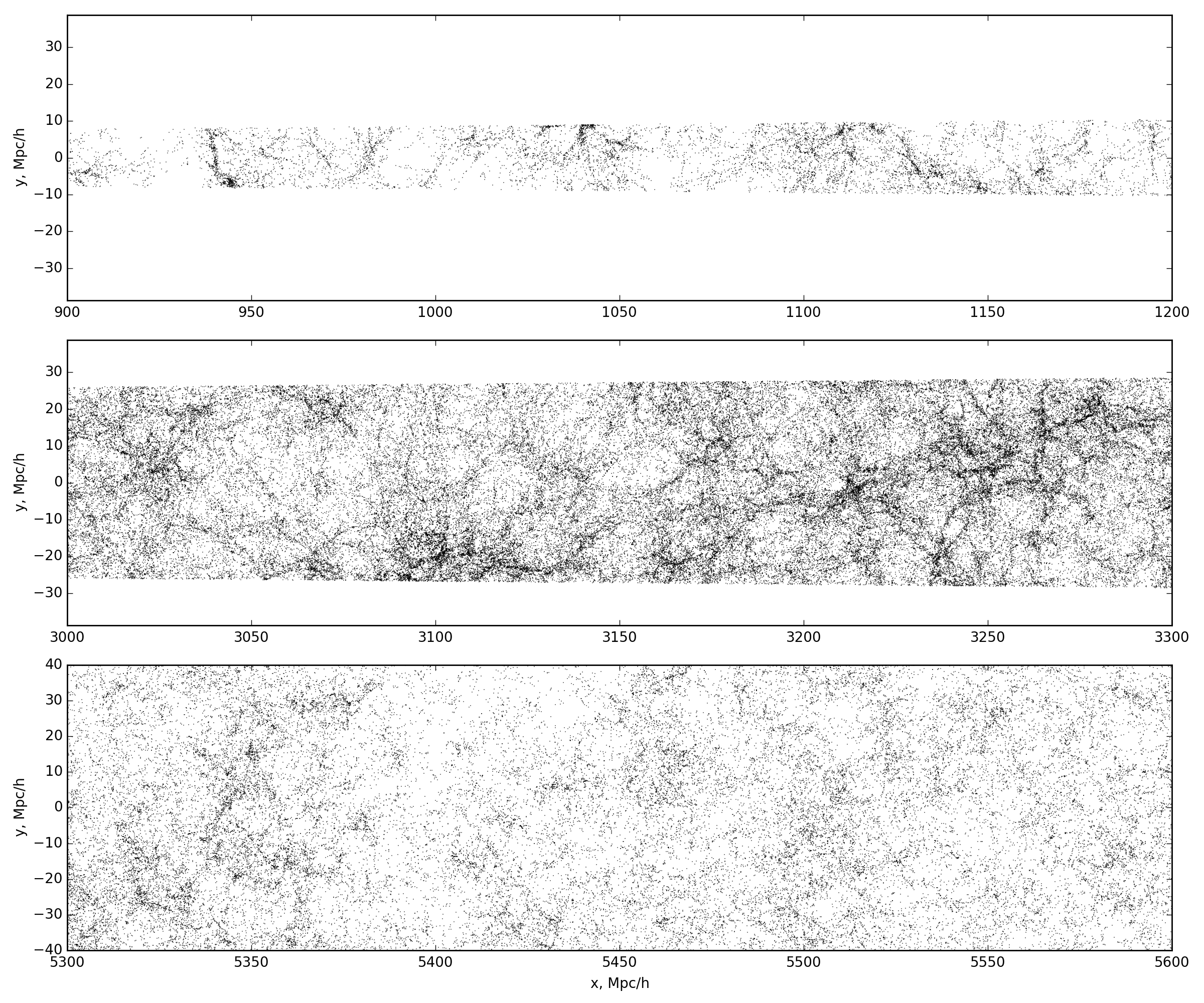
Figure 1: Several regions of the cone projection onto the XY plane in comoving coordinates. The X axis is along the cone axis. Each point is a separate halo.

Table 1: Parameters of the simulated survey cone

Parameter	Value
Minimum redshift	0.30
Maximum redshift	6.19
Minimum mass	$3\times 10^{10}$ $h^{-1}$ M⊙
Maximum mass	$2.56\times 10^{14}$ $h^{-1}$ M⊙
Number of halos	1285307
Number of halos $M>10^{13}$ $h^{-1}$ M⊙	936
Number of halos $M>10^{14}$ $h^{-1}$ M⊙	15

The cone parameters are presented in Table 1. The cone contains 15 clusters of galaxies and $\sim$ 900 groups. To analyze the large-scale structure in this cone, we used the minimal spanning tree technique, which is widely applied in searching for superclusters (Doroshkevich et al., 2004; Pilipenko, 2007; Clowes et al., 2013). In this case, two parameters are specified: the maximum threshold branch length needed to include the branch in a cluster and the minimum number of objects in the cluster. Both parameters were varied. For example, the histogram of the distribution of tree branches in length has a maximum at a length of 0.5 Mpc/$h$. If we take this value as the threshold length and choose 100 objects as the threshold number, then in our catalog the algorithm detects 11 clusters whose size does not exceed 20 Mpc/$h$.

3.3 Gravitaional lensing

To take into account the gravitational lensing, we search for all possible pairs of close (in angular separation) halos in the produced catalog and calculate the magnifications of the more distant halo (source) in this pair from the observer when lensed by the closer halo (lens). The magnifications μ were calculated for two simple lens models: a point lens (PL) and a singular isothermal sphere (SIS). The expression for the magnification is known (see, e.g., Schneider et al. (1992)) to be

$$\mu(M_{L},D_{L},D_{S},\beta)={\tilde{\beta}^{2}+2\over\tilde{\beta}\sqrt{\tilde{\beta}^{2}+4}}$$ (1)

for the PL model and

$$\mu(M_{L},D_{L},D_{S},\beta)=\begin{cases}{2\over\tilde{\beta}},&\tilde{\beta}\leqslant 1\\ {\tilde{\beta}+1\over\tilde{\beta}},&\tilde{\beta}>1\end{cases},$$ (2)

for the SIS model, where

$$\tilde{\beta}={\beta\over\alpha_{0}},$$ (3)

$\beta$ is the angular separation between the source and the lens, $\alpha_{0}$ is the characteristic angular separation dependent on the source redshift $z_{S}$ and the lens redshift $z_{L}$.

The characteristic angular separation $\alpha_{0}$ is written as

$$\alpha_{0}=\sqrt{{4GM_{L}\over c^{2}}{D_{LS}\over D_{S}D_{L}(1+z_{L})}},$$ (4)

where $D_{L}$ and $D_{S}$ are the comoving distances from the observer to the lens and the source, respectively, $D_{LS}$ is the comoving distance between the lens and the source, $z_{L}$ is the lens redshift, $c$ is the speed of light, and $G$ is the gravitational constant (Schneider et al., 1992).

For our purposes, we took into account the strong gravitational lensing events with a magnification $\geq 2$, which subsequently allowed us to properly compare our results for the source counts with those from Béthermin et al. (2011). Furthermore, we took into account the extent of the emission sources. The sources were assumed to be circles with a uniform surface brightness with a radius $\rho$ equal to 0.25 arcsec. In this case, the maximum magnification for the PL model is (Schneider, 1987)

$$\mu_{max}=\frac{\sqrt{\gamma^{2}+4}}{\gamma},\;\;\gamma=\frac{\rho}{\alpha_{0}},$$ (5)

As our calculations show (see Fig. 2), allowance for the strong gravitational lensing events with a magnification $\geq$2 in the SIS model turns out to be important when counting the sources at fluxes larger than 10 mJy for wavelengths of 70, 250, and 500 $\mu$m and larger than 1 mJy at a wavelength of 1.2 mm. In Fig. 2 the solid line and, for comparison, the dotted line indicate, respectively, the results with and without gravitational lensing. The PL model gives slightly poorer agreement with the source counts. In the model of backward evolution from Béthermin et al. (2011), the lensing was also taken into account and similar results were obtained.

3.4 Determining the luminosities of galaxies

In this paper we used one of the most commonly applied relations between halo mass $M$ and galaxy luminosity $L$ from Viero et al. (2013):

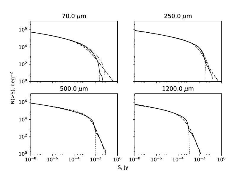
Figure 2: Source counts in our model with gravitational lensing (solid lines), without gravitational lensing (dotted line), and in the model of Béthermin et al. (2011) (dashed line) at 70, 250, 500, and 1200 $\mu$m. The thin dash–dotted line is our model for the case of minimum redshift $z=0.3$.

$$L(M,z)=L_{0}(1+z)^{\eta}\log(M)\exp\left(-{(\log(M)-\log(M_{0}))^{2}\over 2\sigma_{L}^{2}}\right),$$ (6)

where $\log(M_{0})=12.6$, $\sigma_{L}^{2}=0.15$, $\eta=3.16$ at $z<2$ and $\eta=0$ at $z>2$, $L_{0}=5\times 10^{9}$ L_⊙ for the integrated luminosity in the range from 8 to 1000 $\mu$m in the galaxy frame. This mass–luminosity relation is based on the fact that the star formation is most efficient in a limited range of halo masses, near $M_{0}$ (Shang et al., 2012). For masses much higher or lower than this one the star formation is suppressed by the feedback effects: photoionization, supernova explosions, AGN activity (Kereš et al., 2005; Bower et al., 2006; Croton et al., 2006). The model parameters $L_{0}$, $M_{0}$, and $\sigma_{L}$ were determined by fitting the source counts to the results from Béthermin et al. (2011), as the best of the existing fits of the source counts in different ranges. Note that the model of backward evolution from this paper is an updated version of the earlier model proposed in Lagache et al. (2003).

To determine the model parameters $L_{0}$, $M_{0}$ and $\sigma_{L}$, we used the source counts as a function of the flux at $\lambda=$ 70, 110, 160, 250, 350, 500, 850, 1200, and 2000 $\mu$m. The parameters were determined by minimizing the rms deviation of the source counts in the same flux intervals as in the data from Béthermin et al. (2011). The integrated counts were compared for the most accurate reproduction of the faint source counts.

For each wavelength we calculated the monochromatic flux, i.e., no information about the passband was used. Note that the data given in Béthermin et al. (2011) were obtained with real telescopes in finite-width passbands. Fitting these data without allowance for the shape of the passband automatically corrects the parameters of our model in such a way that the results obtained in it are already not monochromatic but those obtained with an averaged passband over all the instruments whose data were used in Béthermin et al. (2011).

The source counts in our model and in the models of Béthermin et al. (2011) are shown in Fig. 2. As can be seen from this figure, good agreement of the results obtained in both models is observed at longer wavelengths, while a discrepancy is observed for fluxes 10–100 mJy at short wavelengths.

3.5 The Spectra of Galaxies

The shape of the spectral energy distribution was taken from Michałowski et al. (2010). The luminosity determined by the method described above specifies its amplitude for each galaxy. Using only one spectrum for all galaxies is a serious simplification of the model. In the approach adopted here each galaxy has its unique halo, and one can devise a large number of ways of specifying the galaxy type as a function of the formation history of this halo, its spatial environment, angular momentum, etc. Analysis of this ways is beyond the scope of this paper. Nevertheless, for comparison we also used several other galaxy spectra that were taken from the library of spectra in Chary & Elbaz (2001), where 105 model spectra are presented. We chose the two extreme spectra, with the largest and smallest fractions of far-IR emission, whereupon the source count fitting procedure was repeated. As a result, the counts changed by no more than 30%, which is comparable to the accuracy of our model.

A consequence of applying a single spectrum for all types of galaxies is a slight spread in galaxy luminosity at fixed mass. This spread is caused by the redshift dependence of the luminosity. For example, galaxies with halo masses of $10^{13}$ M_⊙ and $10^{11}$ M_⊙ have IR luminosities from $10^{10}$ to $10^{11}$ L_⊙ and from $10^{6}$ to $10^{7}$ L_⊙, respectively. The inferred spread is several times smaller than that observed, for example, in SDSS galaxies at low redshifts (Brinchmann et al., 2004).

3.6 Comparison with the ALMA Observations

Recent deep observations at the ALMA observatory (Carniani et al., 2015; Fujimoto et al., 2016) have yielded for the first time the source counts at wavelengths 1.1–1.3 mm with fluxes 20–100 $\mu$Jy. We compared these counts with the predictions of our model; the results are presented in Table 2. As can be seen from this table, the predictions of our model are in good agreement (given the measurement errors) with the ALMA observations.

Table 2: Comparison with the ALMA source counts

Parameter	Observations	Our model
$\lambda=1.1$ mm (Carniani et al., 2015)
Integrated flux at $S>130$ $\mu$Jy	$>17.2$ Jy deg-2	14.8 Jy deg-2
$dN/d(\log_{10}S)$ at $S=130$ $\mu$Jy	$10^{+7}_{-4}\times 10^{4}$ deg-2	$3.5\times 10^{4}$ deg-2
$\lambda=1.3$ mm (Carniani et al., 2015)
Integrated flux at $S>60$ $\mu$Jy	$>12.9$ Jy deg-2	9.5 Jy deg-2
$dN/d(\log_{10}S)$ at $S=60$ $\mu$Jy	$11^{+14}_{-7}\times 10^{4}$ deg-2	$3.8\times 10^{4}$ deg-2
$\lambda=1.2$ mm (Fujimoto et al., 2016)
Integrated flux at $S>20$ $\mu$Jy	$22.9^{+6.7}_{-5.6}$ Jy deg-2	13.1 Jy deg-2
$dN/d(\log_{10}S)$ at $S=20$ $\mu$Jy	$3.2\times 10^{5}$ deg-2	$5.9\times 10^{4}$ deg-2

4 The Identification of Point Sources and the Confusion Limit

There exist at least two criteria for determining the confusion limit (Dole et al., 2003): the photometric and source density criteria. The photometric criterion is applied to sources that are too faint to be detected separately. In contrast, the source density criterion is applied to sources that can be detected as individual objects. Given a simulated sky map, it is also possible to study the completeness of the catalog of point sources extracted from this map. This method is closest to real measurements. Nevertheless, the result can depend on the applied source identification algorithm.

In this paper the confusion limit was determined using the following four methods.

(1) The source density criterion. For sources with a flux above some threshold value the probability of having two sources in the telescope beam is less than 10% (Dole et al., 2003):

$$N_{\mathrm{SDC}}(>S_{\mathrm{lim}})=-{\log(1-P)\over\pi k^{2}\theta_{FW}^{2}},$$ (7)

where $N_{\mathrm{SDC}}(>S_{\mathrm{lim}})$ is the density of sources with a flux above the threshold value $>S_{\mathrm{lim}}$, $\theta_{FW}$ is the full width at half maximum of the beam profile, $P$ is the probability that the two sources will be indistinguishable, i.e., will be at a distance less than $k\theta_{FW}$, where $k=0.8$. As can be seen, only the information about the source counts is sufficient for this criterion to be applied.

(2) The photometric criterion:

$$S_{\mathrm{lim}}=q\sigma(S_{\mathrm{lim}}),$$ (8)

where $\sigma(S_{\mathrm{lim}})$ is the level of flux fluctuations in the telescope beam from sources with a flux below the threshold value $S_{\mathrm{lim}}$, $q=5$ is the signal-to-noise ratio needed for successful detection. The value of $\sigma(S_{\mathrm{lim}})$ can be found in two ways: from the source counts by assuming their uniform random distribution and directly from the simulated map.

(3) The photometric criterion with the determination of $\sigma(S_{\mathrm{lim}})$ from a simulated map containing no sources brighter than $S_{\mathrm{lim}}$.

(4) Investigation of the map completeness. It consists in determining the flux at which the fraction of the sources found among those initially included in the model will be 50%. The search for sources on the maps was made by several methods. The first of them is to determine the local maxima using the second derivatives (we used the code provided to us by D.I. Novikov). This method yields good results for a noiseless map, but it cannot be applied for real astronomical images. The result of the identification of point sources by this method is shown in Fig. 3.

We used two more methods widely applied in practice. One of them, SEXTRACTOR (Bertin & Arnouts, 1996), found much fewer sources than did the method of local maxima; therefore, we abandoned this method. The second one is the getsources code applied to process the images from the Herschel space observatory (Men’shchikov et al., 2012). This code has two modes: the monochromatic one, where the map only at one wavelength is used, and the multiwavelength one. In the latter the map with the best angular resolution (usually in the shortest wavelength range) is used to determine the coordinates of sources on the remaining maps. Getsources showed excellent results comparable to those of the method of local maxima in the monochromatic mode, while in the multiwavelength mode it surpassed the method of maxima.

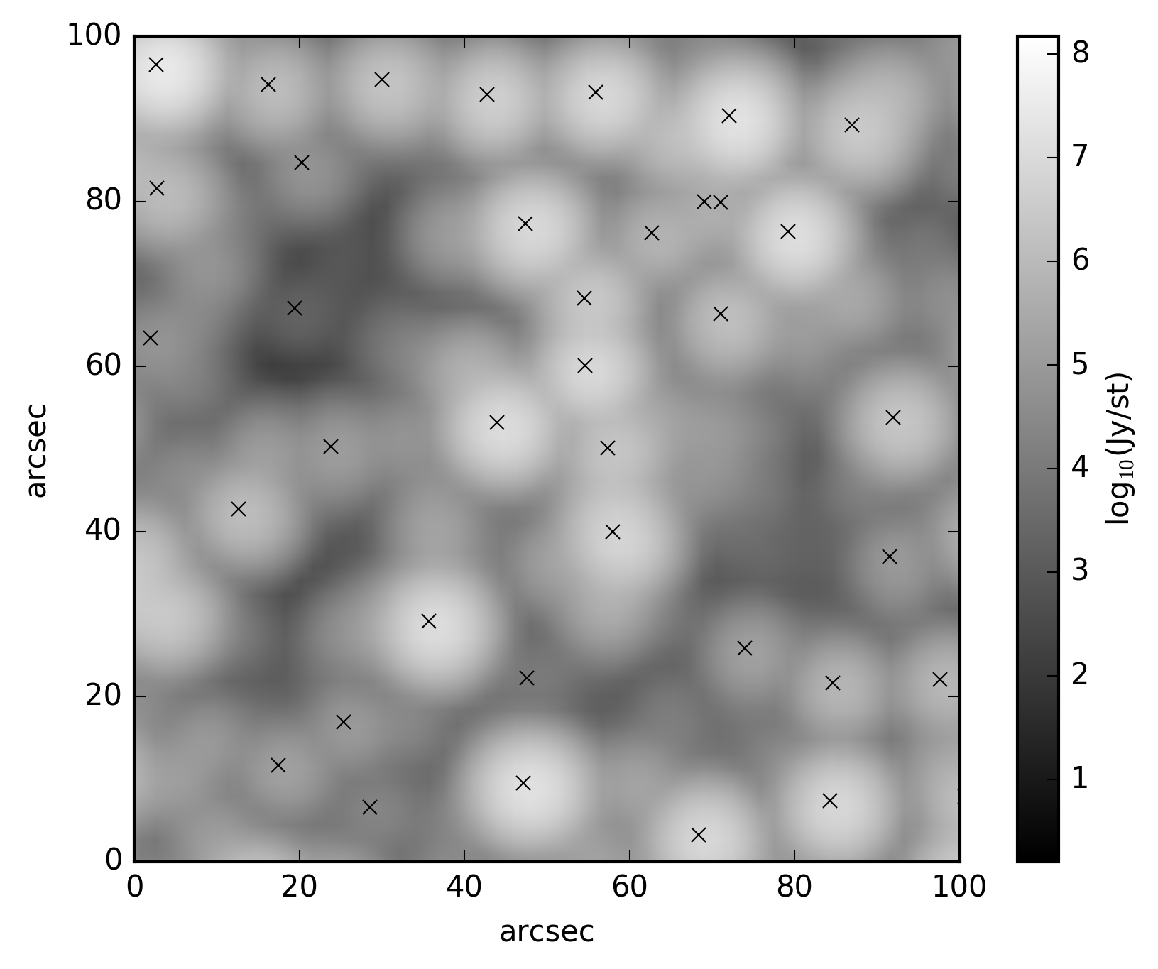
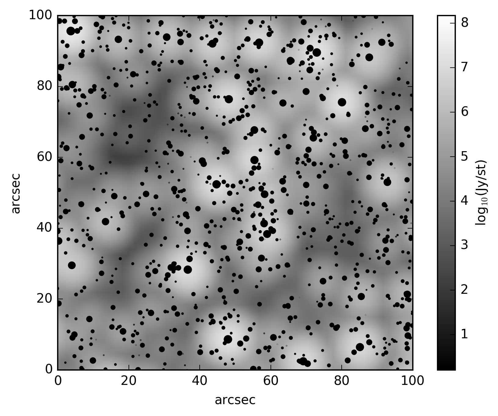
Figure 3: Example of a $100^{\prime\prime}\times 100$ field of the simulated sky background map at 300 $\mu$m. The crosses on the left indicate the intensity peaks found using the second derivatives. The dots on the right indicate the model galaxies. The dot size is proportional to the logarithm of the galaxy flux.

Figure 3 illustrates the confusion problem, where the distribution of model galaxies in the sky field is shown on the right. After convolution with the telescope beam, the brightest galaxies create aureoles around themselves that exceed considerably $\lambda/D=6$” in their sizes and in which the emission from the neighboring fainter galaxies is lost. As a result, the intensity peaks on the CIB map (in Fig. 3 on the left) correspond to the brightest galaxies.

The results of determining the confusion limits for two telescope apertures, 3.5 m (Herschel) and 10 m (Millimetron), for the four above-listed criteria are presented in Table 3. It can be seen from this table that the confusion limits for the 3.5-m telescope predicted in our model according to the completeness criterion are close to those actually found from the Herschel observations. For example, the confusion limit is 5.8 mJy for the SPIRE instrument at 250 $\mu$m (Nguyen et al., 2010) and 0.27 mJy for the PACS instrument at 100 $\mu$m (Tuttlebee, 2013).

To determine the accuracy of finding the confusion limit from the simulated maps, we divided the maps into four equal regions and found the confusion limit in each of them. The deviation from the limit for the complete map turned out to be 60% for all ranges and apertures from Table 3.

Table 3: Confusion limits in the far-IR/submillimeter range

Aperture/criterion	100 $\mu$m	300 $\mu$m	1000 $\mu$m
3.5 m (Herschel)
Source density	80 $\mu$Jy	10 mJy	3 mJy
Photometric (from counts)	0	6 mJy	5 mJy
Photometric (from map)	60 $\mu$Jy	20 mJy	13 mJy
Completeness 50%:
search for maxima	0.2 mJy	9 mJy	4 mJy
getsources monochromatic	0.5 mJy	14 mJy	12 mJy
getsources multiwavelength	0.5 mJy	3 mJy	2 mJy
10 m (Millimetron)
Source density	1 nJy	0.3 mJy	1 mJy
Photometric (from counts)	0	0.3 $\mu$Jy	1 mJy
Photometric (from map)	40 $\mu$Jy	0.3 mJy	4 mJy
Completeness 50%:
search for maxima	14 $\mu$Jy	0.6 mJy	1 mJy
getsources monochromatic	9 $\mu$Jy	0.7 mJy	1 mJy
getsources multiwavelength	10 $\mu$Jy	0.1 mJy	1 mJy

We see that at 100 $\mu$m the photometric criterion calculated from the source counts gives zero confusion limit. In addition, for the 10-m telescope at 300 $\mu$m the two photometric criteria give values differing by three orders of magnitude. This is because the dependence $\sigma(S_{\mathrm{lim}})$ in some ranges of fluxes is nearly linear, and a small shift leads to the disappearance of the solution of Eq. (8). The photometric criterion uses only the tail of the distribution with the lowest fluxes while disregarding the resolved sources whose density in the sky is, nevertheless, quite high. Therefore, in the case where the confusion limit according to the photometric criterion approaches zero, other criteria should be used.

To check the influence of the large-scale structure on confusion, we mixed the coordinates of galaxies in the sky, leaving the fluxes from them unchanged. Within the accuracy of our method no difference was found for all the methods of determining the confusion limit presented in Table 3.

5 The Large-Scale Structure

The CIB is known to be anisotropic. For example, a study of the spatial anisotropy power spectrum obtained from the Herschel observations in Viero et al. (2013) showed that this spectrum could be explained in terms of the analytical halo clustering model. The constructed power spectrum for the simulated CIB maps obtained in our model for the 3.5-m aperture is compared with the power spectrum from Viero et al. (2013). These spectra are shown in Fig. 4. To construct them, we subtracted the shot-noise contribution from the power spectrum of the spatial background anisotropy while taking into account the telescope beam.

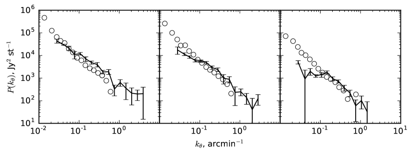
Figure 4: Power spectrum of the spatial sky CIB anisotropy at 250, 350, and 500 $\mu$m (from left to right). The circles are the results from Viero et al. (2013) (no errors are shown); the solid line indicates our results.

As can be seen from Fig. 4, our model success- fully reproduces the background anisotropy spectrum within the measurement error limits (the measurement errors at the Herschel telescope are not shown in Fig. 4). The slight systematic differences may stem from the fact that our map processing procedure differs from that used in Viero et al. (2013). In particular, to remove the shot noise, we produced the maps without anisotropy where the source coordinates were random, while their fluxes did not change compared to the map with a structure.

It is important to note that in our model the elements of the three-dimensional large-scale structure observed in the distribution of halos in space can be directly compared with the clusters of spots on the CIB map. For our cluster analysis we used the minimal spanning tree technique. We varied the threshold length for three-dimensional clusters by choosing it from the set of 0.3, 0.5, and 1.0 Mpc and the minimum mass as 30, 100, or 500 objects, respectively. We identified all peaks on the map with a brightness twice as high as the confusion limits that we deter- mined from the 50% completeness criterion at 100 and 300 $\mu$m. Among these peaks we found clusters with threshold branch lengths of 20”, 25”, and 30” using the same minimal spanning tree algorithm; the number of peaks is 10, 30, and 100, respectively. Next, for all identifications of three-dimensional clusters and all identifications of cluster peaks we performed a cross-identification by their locations in the sky. As a rule, one or more overlapping clusters were observed. The probability of a chance coincidence was determined by cyclically shifting one of the maps by a random vector. As a result, it emerged that the probability of a chance realization of the observed coincidences at the parameters we use is at least 5%, suggesting that there is no correspondence between the maps of peaks in the CIB and three-dimensional superclusters of galaxies.

6 Conclusions

We constructed a semi-analytical model of the sky CIB whose new element is allowance for the data from cosmological simulations of the large-scale structure of the Universe and the construction of simulated CIB maps to which various source searching algorithms can be applied. The developed model shows good agreement with the known data on source counts and the power spectrum of the spatial CIB anisotropy in the wavelength range from 100 $\mu$m to 2 mm. This model was used to determine the confusion limit for future 10-m far-IR space telescopes and to compare the clustering of background intensity peaks with the actual large-scale structure.

Based on the source counts, we used the source density criterion and the photometric criterion to estimate the confusion limit. The confusion limits obtained with these criteria were compared between themselves and with the confusion limit obtained directly from the CIB map using the completeness criterion. In the wavelength range 300–1000 $\mu$m all of the methods used showed close values of the confusion limit, while for a wavelength of 100 $\mu$m the results of the two estimation criteria differ significantly. Furthermore, for the same wavelength, 100 $\mu$m, these estimation criteria yielded a result significantly differing from that obtained by a direct measurement from the background map. It is important to note that the confusion limits for a 3.5-m telescope obtained with the completeness criterion from the simulated map turned out to be close to those found from the observations with the Herschel telescope. Hence it can be concluded that at a telescope aperture of 3–10 m the estimation criteria work well at comparatively long wavelengths, $\lambda\geq 300$, and poorly at short ones.

At wavelengths of $\sim$100 $\mu$m it will be possible to identify compact sources with a flux density above 10 $\mu$Jy from the maps obtained in the mode of broad-band photometry with a 10-m telescope; this is better than that for a telescope with a mirror diameter of 3.5 m by more than an order of magnitude. For a wavelength of 300 $\mu$m, at which the CIB intensity is at a maximum, the confusion limit will be about 0.6 mJy, which is also lower than the confusion limit measured with the Herschel telescope by an order of magnitude. For a wavelength of 1 mm a 10-m telescope gives a fourfold gain in confusion limit, reaching 1 mJy.

The CIB in our model demonstrates significant deviations from a uniform random distribution of sources in the sky. In this case, the constructed power spectrum of the spatial background anisotropy within the developed model shows good agreement with the power spectrum obtained from the Herschel observations. Thus, the large-scale structure of the Universe clearly manifests itself on the CIB maps. At the same time, the large-scale structure has no noticeable influence on the confusion limit found from the simulated maps.

Our model has demonstrated for the first time that the fluctuations in the number of intensity peaks ob- served in a 1${}^{\circ}\times 1^{\circ}$ field show no clear correlation with superclusters of galaxies. It is necessary to invoke spectroscopic information, for example, to use [CII] and CO lines, to identify the three-dimensional large-scale structure.

Various ways of breaking the confusion limit are considered in the literature: Raymond et al. (2010) assessed the true viability of using spectroscopic information to reduce the confusion on the planned Japanese SPICA space telescope. Safarzadeh et al. (2014) studied the possibility of using optical information to reduce the confusion in the far IR on Herschel images. It is necessary to carry out such studies for Millimetron and other planned observatories, for which purpose our developed model is planned to be used.

7 Acknowledgements

The CosmoSim database used in this paper is a service provided by the Leibnitz Institute for Astrophysics Potsdam. We thank the Gauss Centre for Supercomputing (www.gauss-centre.eu) and the Partnership for Advanced Computing in Europe (PRACE, www.prace-ri.eu) for supporting the MultiDark project of numerical simulations and for providing the computational time for it at GCS Supercomputer SuperMUC at the Leibnitz Rechenzentrum (LRZ, www.lrz.de).

The work of S.V. Pilipenko, M.V. Tkachev, A.A. Ermash, E.V. Mikheeva, and V.N. Lukash was supported by the Russian Foundation for Basic Research grant no. 16-02-01043. The work of M.V. Tkachev was also supported by the Russian Foundation for Basic Research grant no. 16-32-00263. The work was supported by the Basic Research Program P-7 of the Presidium of the Russian Academy of Sciences and grant no. NSh-6595.2016.2 from the President of the Russian Federation for Support of Leading Scientific Schools.

References

- Bertin & Arnouts (1996) Bertin E., Arnouts S., 1996, A&AS, 117, 393
- Béthermin et al. (2011) Béthermin M., Dole H., Lagache G., Le Borgne D., Penin A., 2011, A&A, 529, A4
- Béthermin et al. (2012) Béthermin M., et al., 2012, ApJ, 757, L23
- Bouché et al. (2010) Bouché N., et al., 2010, ApJ, 718, 1001
- Bower et al. (2006) Bower R. G., Benson A. J., Malbon R., Helly J. C., Frenk C. S., Baugh C. M., Cole S., Lacey C. G., 2006, MNRAS, 370, 645
- Brinchmann et al. (2004) Brinchmann J., Charlot S., White S. D. M., Tremonti C., Kauffmann G., Heckman T., Brinkmann J., 2004, MNRAS, 351, 1151
- Carniani et al. (2015) Carniani S., et al., 2015, A&A, 584, A78
- Cattaneo et al. (2005) Cattaneo A., Blaizot J., Devriendt J., Guiderdoni B., 2005, MNRAS, 364, 407
- Cattaneo et al. (2006) Cattaneo A., Dekel A., Devriendt J., Guiderdoni B., Blaizot J., 2006, MNRAS, 370, 1651
- Chary & Elbaz (2001) Chary R., Elbaz D., 2001, ApJ, 556, 562
- Clowes et al. (2013) Clowes R. G., Harris K. A., Raghunathan S., Campusano L. E., Söchting I. K., Graham M. J., 2013, MNRAS, 429, 2910
- Cole et al. (2000) Cole S., Lacey C. G., Baugh C. M., Frenk C. S., 2000, MNRAS, 319, 168
- Conroy & Wechsler (2009) Conroy C., Wechsler R. H., 2009, ApJ, 696, 620
- Cousin et al. (2015) Cousin M., Lagache G., Bethermin M., Blaizot J., Guiderdoni B., 2015, A&A, 575, A32
- Croton et al. (2006) Croton D. J., et al., 2006, MNRAS, 365, 11
- Devriendt & Guiderdoni (2000) Devriendt J. E. G., Guiderdoni B., 2000, A&A, 363, 851
- Dole et al. (2003) Dole H., Lagache G., Puget J.-L., 2003, ApJ, 585, 617
- Domínguez et al. (2011) Domínguez A., et al., 2011, MNRAS, 410, 2556
- Doroshkevich et al. (2004) Doroshkevich A., Tucker D. L., Allam S., Way M. J., 2004, A&A, 418, 7
- Franceschini et al. (2010) Franceschini A., Rodighiero G., Vaccari M., Berta S., Marchetti L., Mainetti G., 2010, A&A, 517, A74
- Fujimoto et al. (2016) Fujimoto S., Ouchi M., Ono Y., Shibuya T., Ishigaki M., Nagai H., Momose R., 2016, ApJS, 222, 1
- Granato et al. (2004) Granato G. L., De Zotti G., Silva L., Bressan A., Danese L., 2004, ApJ, 600, 580
- Gruppioni et al. (2011) Gruppioni C., Pozzi F., Zamorani G., Vignali C., 2011, MNRAS, 416, 70
- Guiderdoni et al. (1998) Guiderdoni B., Hivon E., Bouchet F. R., Maffei B., 1998, MNRAS, 295, 877
- Henriques et al. (2013) Henriques B. M. B., White S. D. M., Thomas P. A., Angulo R. E., Guo Q., Lemson G., Springel V., 2013, MNRAS, 431, 3373
- Hopkins et al. (2008) Hopkins P. F., Hernquist L., Cox T. J., Kereš D., 2008, ApJS, 175, 356
- Jeong et al. (2006) Jeong W.-S., Pearson C. P., Lee H. M., Pak S., Nakagawa T., 2006, MNRAS, 369, 281
- Kardashev et al. (2014) Kardashev N. S., et al., 2014, Physics Uspekhi, 57, 1199
- Kereš et al. (2005) Kereš D., Katz N., Weinberg D. H., Davé R., 2005, MNRAS, 363, 2
- Klypin et al. (2016) Klypin A., Yepes G., Gottlöber S., Prada F., Heß S., 2016, MNRAS, 457, 4340
- Lacey et al. (2010) Lacey C. G., Baugh C. M., Frenk C. S., Benson A. J., Orsi A., Silva L., Granato G. L., Bressan A., 2010, MNRAS, 405, 2
- Lagache et al. (2003) Lagache G., Dole H., Puget J.-L., 2003, MNRAS, 338, 555
- Lonsdale (1996) Lonsdale C., 1996, in Dwek E., ed., American Institute of Physics Conference Series Vol. 348, American Institute of Physics Conference Series. pp 147–158
- Men’shchikov et al. (2012) Men’shchikov A., André P., Didelon P., Motte F., Hennemann M., Schneider N., 2012, A&A, 542, A81
- Michałowski et al. (2010) Michałowski M., Hjorth J., Watson D., 2010, A&A, 514, A67
- Negrello et al. (2010) Negrello M., et al., 2010, Science, 330, 800
- Nguyen et al. (2010) Nguyen H. T., et al., 2010, A&A, 518, L5
- Pilipenko (2007) Pilipenko S. V., 2007, Astronomy Reports, 51, 820
- Rahmati & van der Werf (2011) Rahmati A., van der Werf P. P., 2011, MNRAS, 418, 176
- Raymond et al. (2010) Raymond G., Isaak K. G., Clements D., Rykala A., Pearson C., 2010, PASJ, 62, 697
- Rowan-Robinson (2009) Rowan-Robinson M., 2009, MNRAS, 394, 117
- Safarzadeh et al. (2014) Safarzadeh M., et al., 2014, in American Astronomical Society Meeting Abstracts #223. p. 433.06
- Schneider (1987) Schneider P., 1987, A&A, 179, 71
- Schneider et al. (1992) Schneider P., Ehlers J., Falco E. E., 1992, Gravitational Lenses, doi:10.1007/978-3-662-03758-4.
- Shang et al. (2012) Shang C., Haiman Z., Knox L., Oh S. P., 2012, MNRAS, 421, 2832
- Smirnov et al. (2012) Smirnov A. V., et al., 2012, in Space Telescopes and Instrumentation 2012: Optical, Infrared, and Millimeter Wave. p. 84424C, doi:10.1117/12.927184
- Tuttlebee (2013) Tuttlebee M., 2013, HERSCHEL/PLANCK Star Tracker Performance Assessment and Calibration, PT-CMOC-OPS-RP-6435-HSO-GF
- Valiante et al. (2009) Valiante E., Lutz D., Sturm E., Genzel R., Chapin E. L., 2009, ApJ, 701, 1814
- Vieira et al. (2013) Vieira J. D., et al., 2013, Nature, 495, 344
- Viero et al. (2013) Viero M. P., et al., 2013, ApJ, 779, 32
- Weinmann et al. (2012) Weinmann S. M., Pasquali A., Oppenheimer B. D., Finlator K., Mendel J. T., Crain R. A., Macciò A. V., 2012, MNRAS, 426, 2797
- Wild et al. (2009) Wild W., et al., 2009, Experimental Astronomy, 23, 221