Abstract

We tackle highly nonconvex, nonsmooth composite optimization problems whose objectives comprise a Moreau-Yosida regularized term. Classical nonconvex proximal splitting algorithms, such as nonconvex ADMM, suffer from lack of convergence for such a problem class. To overcome this difficulty, in this work we consider a lifted variant of the Moreau-Yosida regularized model and propose a novel multiblock primal-dual algorithm that intrinsically stabilizes the dual block. We provide a complete convergence analysis of our algorithm and identify respective optimality qualifications under which stationarity of the original model is retrieved at convergence. Numerically, we demonstrate the relevance of Moreau-Yosida regularized models and the efficiency of our algorithm on robust regression as well as joint feature selection and semi-supervised learning.

1 Introduction

We are interested in the solution of the nonconvex, Moreau-Yosida regularized consensus minimization problem

$$\underset{\begin{subarray}{c}u\in\mathbb{R}^{n},~{}v\in\mathbb{R}^{m}\end{subarray}}{\text{minimize}} \textstyle e_{\lambda}f(v)+g(u)$$ (1)

subject to $$Au=v,$$

where $e_{\lambda}f$ is the Moreau envelope [18] of $f$ with parameter $\lambda>0$.

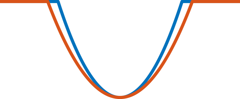
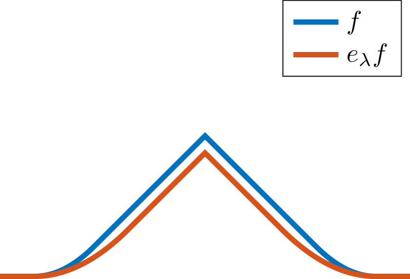
Figure 1: Illustration of nonconvex, nonsmooth Moreau envelopes $e_{\lambda}f$ (red curves). The two depicted piecewise quadratic loss functions $f$ (blue curves), are invariant under Moreau-Yosida regularization up to rescaling. Left: The Moreau envelope of a truncated quadratic loss, given as $f=\min\;\{\nu,(\cdot)^{2}\}$ for $\nu>0$, is a nonsmooth, nonconvex truncated quadratic loss with rescaled slope. Right: The Moreau envelope of a symmetric Huberized hinge loss is a nonsmooth, nonconvex symmetric Huberized hinge loss with rescaled slopes of the quadratic pieces given as $e_{\lambda}f=\min_{\theta\in\{-1,1\}}e_{\lambda}(1-(\cdot)\theta)_{+}$.

The extended real-valued functions, $f$ and $g$, are assumed to be proper, lower semi-continuous (lsc), and in general nonconvex. The block variables $u$ and $v$ are separated in the objective, but comply with a consensus constraint for matrix $A\in\mathbb{R}^{m\times n}$.

To argue that model (1) is relevant in statistics and machine learning we briefly review some general properties of the Moreau envelope, formally defined as follows.

Definition 1 (Moreau envelope and proximal mapping).

For a proper, lsc function $f:\mathbb{R}^{m}\to\mathbb{R}\cup\{\infty\}$ and parameter $\lambda>0$, the Moreau envelope function $e_{\lambda}f$ and the proximal mapping $P_{\lambda}f$ are defined by

$$e_{\lambda}f(v) :=\inf_{z\in\mathbb{R}^{m}}f(z)+\frac{1}{2\lambda}\|z-v\|^{2},$$

$$P_{\lambda}f(v) :=\operatorname*{arg\,min}_{z\in\mathbb{R}^{m}}f(z)+\frac{1}{2\lambda}\|z-v\|^{2}.$$

For convex $f$, the Moreau envelope $e_{\lambda}f$ yields a convex and smooth lower approximation to $f$, cf. [22, Theorem 2.26]. In contrast, for nonconvex nonsmooth $f$ the Moreau envelope $e_{\lambda}f$ remains nonsmooth and nonconvex in general which renders its optimization challenging. In fact, many nonsmooth, nonconvex objectives in machine learning tasks, such as semi-supervised Huber-SVMs, or robust regression are even invariant, up to different choices of $\lambda$, under Moreau-Yosida regularization. This is exemplarily illustrated for the truncated quadratic loss [23, 16], and the “symmetric Huberized hinge loss” [2, 12, 6] in Figure 1, where Moreau-Yosida regularization preserves nonsmoothness and nonconvexity of $f$.

For $e_{\lambda}f$ smooth and $g$ nonsmooth, problems of the form (1) can be optimized by proximal splitting methods such as (accelerated) proximal gradient methods [19, 21], or primal-dual algorithms such as the alternating direction method of multipliers (ADMM) [10, 9, 8, 7, 11, 14, 24]. All these algorithms typically update the block variables in a Gauss-Seidel fashion, and exploit efficient evaluation of the proximal mapping of $e_{\lambda}f$ or $g$. Proximal splitting methods are traditionally applied for convex optimization, in which case their convergence is guaranteed without smoothness of the objective. More recently, convergence of ADMM is extended to certain nonconvex settings [11, 14, 24], but the convergence analysis requires, e.g., that $e_{\lambda}f$ is Lipschitz differentiable. In some sense, convexity is traded off against smoothness in a convergent algorithm. However, when both $e_{\lambda}f$ and $g$ in (1) are nonsmooth and nonconvex (as encountered in numerous machine learning applications), the proximal gradient method is inapplicable and the ADMM is non-convergent.

To overcome such difficulties, we propose a novel multiblock primal-dual scheme for solving problem (1). Our contributions are summarized as follows:

• We devise a novel multiblock primal-dual scheme in Section 2.1, and prove its subsequential convergence to a critical point of the lifted representation of problem (1) in Section 3.

• We draw connections of our primal-dual algorithm to a fully primal coordinate descent on a quadratic penalty function; see Section 2.2.

• For piecewise smooth, piecewise convex functions of the form $\min_{i\in\mathcal{I}}e_{\lambda}f_{i}$ (as a subfamily of nonconvex, nonsmooth functions), we identify an optimality qualification related to active set, under which a critical point of the lifted problem translates to a critical point of (1); see Section 4.2. For a specific choice of the step size, we show that our optimality qualification is guaranteed to hold.

• We experimentally validate our proposed algorithm on robust regression as well as joint feature selection and semi-supervised learning in Section 5. In comparison with classical nonconvex ADMM, our method consistently performs favorably in terms of lower objective value and vanishing optimality gap.

2 A Multiblock Primal-Dual Method

2.1 Derivation

For $e_{\lambda}f$ smooth, the convergence of ADMM in the nonconvex setting is shown via a monotonic decrease of the augmented Lagrangian [11], which serves as a Lyapunov function. As a key step in the proof of [11], the ascent of the augmented Lagrangian, caused by the dual update, is dominated by a sufficient descent in the primal block that is updated last.

In order to recover convergence for nonsmooth $e_{\lambda}f$, we employ a lifting of the problem which yields a third primal block in the optimization. More precisely, we introduce new variables $z,w$ along with a linear constraint

$$z+w=v,$$ (2)

and integrate the Moreau-Yosida regularization into the lifted problem:

$$\underset{\begin{subarray}{c}u\in\mathbb{R}^{n},~{}w,z\in\mathbb{R}^{m}\end{subarray}}{\text{minimize}} f(z)+\frac{1}{2\lambda}\|w\|^{2}+g(u)$$ (3)

subject to $$Au-z-w=0.$$

To this lifted problem we apply the following multiblock primal-dual scheme, where the block $w$, updated last, corresponds to the smooth function $\frac{1}{2\lambda}\|\cdot\|^{2}$ that realizes the Moreau-Yosida regularization. Let the augmented Lagrangian of the problem be defined as

$$\mathfrak{L}_{\rho}(u,z,w,y)=f(z)+g(u)+\frac{1}{2\lambda}\|w\|^{2}$$ (4)

$$\qquad+\langle y,Au-z-w\rangle+\frac{\rho}{2}\|Au-z-w\|^{2},$$

for $\rho>0$. Also let $M:=\frac{1}{\sigma}I-\rho A^{\top}A$, which is positive definite for $\sigma\rho\|A\|^{2}<1$, and $\|\cdot\|_{M}:=\sqrt{\langle\cdot,M\cdot\rangle}$. Then our scheme is formulated as

$$u^{t+1} \in\textstyle\operatorname*{arg\,min}_{u}\mathfrak{L}_{\rho}(u,z^{t},w^{t},y^{t})+\frac{1}{2}\|u-u^{t}\|_{M}^{2},$$ (5)

$$z^{t+1} \in\textstyle\operatorname*{arg\,min}_{z}\mathfrak{L}_{\rho}(u^{t+1},z,w^{t},y^{t}),$$

$$w^{t+1} =\textstyle\operatorname*{arg\,min}_{w}\mathfrak{L}_{\rho}(u^{t+1},z^{t+1},w,y^{t}),$$

$$y^{t+1} =y^{t}+\rho(Au^{t+1}-z^{t+1}-w^{t+1}).$$

Motivated by [5, 15] we include a proximal term $\frac{1}{2}\|u-u^{t}\|_{M}^{2}$ to guarantee tractability of the subproblem for the $u$-update, as long as the proximal mapping of $g$ is simple. Once rephrasing the update of $u$ in terms of a proximal mapping as $u^{t+1}=\textstyle P_{\sigma}g(u^{t}-\sigma A^{\top}(y^{t}+\rho(Au^{t}-z^{t}-\lambda y^{t})))$, one can interpret it as a proximal gradient descent step on the augmented Lagrangian.

The optimality condition for the last primal block update $0\stackrel{{\scriptstyle!}}{{=}}\frac{1}{\lambda}w^{t+1}-y^{t}-\rho(Au^{t+1}-z^{t+1}-w^{t+1})$ matches the dual update and shows that $w$ is equal to the dual variable up to scaling, i.e., $\lambda y^{t+1}=w^{t+1}$. Therefore, the variable $w$ can be eliminated from the algorithm, and we arrive at a compact formulation of the proposed multiblock primal-dual scheme, i.e., Algorithm 1, for Moreau-Yosida regularized problems.

Algorithm 1 (multiblock primal-dual scheme).

Choose $\rho,\sigma$ such that $\rho\lambda>1$ and $\sigma\rho\|A\|^{2}<1$. For $t=1,2,\dots$ do $\displaystyle u^{t+1}$ $\displaystyle\in\textstyle P_{\sigma}g\left(u^{t}-\sigma A^{\top}(y^{t}+\rho(Au^{t}-z^{t}-\lambda y^{t}))\right),$ $\displaystyle z^{t+1}$ $\displaystyle\in\textstyle P_{\nicefrac{{1}}{{\rho}}}f\left(Au^{t+1}+(\nicefrac{{1}}{{\rho}}-\lambda)y^{t}\right),$ $\displaystyle y^{t+1}$ $\displaystyle=\tfrac{1}{1+\rho\lambda}(y^{t}+\rho(Au^{t+1}-z^{t+1})).$

Note that the lifted problem is equivalent to problem (1) in terms of global minimizers but in general not in terms of critical points. Yet, we show in Section 4 that under mild assumptions, e.g., for piecewise convex piecewise smooth $e_{\lambda}f$, limit points produced by this algorithm translate to critical points of the original problem (1) by reversing the substitution (2). As a side remark, with $\lambda=0$ we arrive at a proximal variant of ADMM [5, 15] also referred to as linearized ADMM, applied to the unregularized problem

$$\underset{\begin{subarray}{c}u\in\mathbb{R}^{n},~{}v\in\mathbb{R}^{m}\end{subarray}}{\text{minimize}} f(v)+g(u)$$ (6)

subject to $$Au=v.$$

2.2 Primal Optimization as a Special Case

Finally, we draw a connection between Algorithm 1 and existing, fully primal alternating minimization schemes applied to the quadratic penalty

$$Q(u,z)=f(z)+g(u)+\frac{1}{2\lambda}\|Au-z\|^{2},$$ (7)

that corresponds to the unregularized problem (6). For a non-admissible choice of the step size $\nicefrac{{1}}{{\rho}}=\lambda$, the Lagrange multiplier $y^{t}$ in Algorithm 1 becomes obsolete and we arrive at Algorithm 2, a fully primal Gauss-Seidel minimization of (7) over $u,z$.

Algorithm 2 (proximal penalty method).

Choose $\tau,\sigma>0$ such that $\sigma\|A\|^{2}<\lambda$. For $t=1,2,\dots$ do $\displaystyle u^{t+1}$ $\displaystyle\in\textstyle P_{\sigma}g\left(u^{t}-\nicefrac{{\sigma}}{{\lambda}}A^{\top}(Au^{t}-z^{t}))\right),$ $\displaystyle z^{t+1}$ $\displaystyle\in\textstyle P_{\lambda}f\left(Au^{t+1}\right).$

The above algorithm appears similar in form to proximal alternating linearized minimization (PALM) [4] applied to (7), where $H(u,z):=\frac{1}{2\lambda}\|Au-z\|^{2}$ is interpreted as the differentiable coupling term. To update $z$, PALM invokes a second proximal gradient descent step on (7) with step size $\tau<\lambda$, i.e., $z^{t+1}=\textstyle P_{\tau}f(z^{t}+\frac{\tau}{\lambda}(Au^{t+1}-z^{t}))$. With the non-admissible step size $\tau=\lambda$, we recast Algorithm 2 from PALM.

3 Convergence Analysis

Our convergence proof borrows arguments from [11], where the convergence of ADMM was shown via a monotonic decrease of the augmented Lagrangian. In our case a Lyapunov function that monotonically decreases over the iterations is obtained by eliminating the variable $w$ from the augmented Lagrangian (4):

$$\mathfrak{Q}_{\rho}(u,z,y)=f(z)-\frac{\lambda}{2}\|y\|^{2}+g(u)$$ (8)

$$\qquad+\langle Au-z,y\rangle+\frac{\rho}{2}\|Au-z-\lambda y\|^{2}.$$

The following lemma is the central part of our convergence proof, as it guarantees convergence of $\mathfrak{Q}_{\rho}(u^{t},z^{t},y^{t})$. Our algorithm has three blocks and invokes a proximal gradient descent step on $\mathfrak{Q}_{\rho}(\cdot,z^{t},y^{t})$ to update $u$. This keeps all block variable updates computationally tractable, as long as the proximal mappings of $f$ and $g$ are simple.

Lemma 1.

Let $\lambda>0$. Choose $\rho>0$ sufficiently large so that $\lambda\rho\geq 1$, and then $\sigma>0$ sufficiently small so that $\sigma\rho\|A\|^{2}<1$. Assume that $e_{\lambda}f(A\,\cdot)+g(\cdot)$ is bounded from below. Then the following statements hold true:

1. $\mathfrak{Q}_{\rho}(u^{t+1},z^{t+1},y^{t+1})$ is an upper bound of the quadratic penalty (7) at $(u^{t+1},z^{t+1})$, i.e.,

   $$Q(u^{t+1},z^{t+1})\leq\mathfrak{Q}_{\rho}(u^{t+1},z^{t+1},y^{t+1}).$$

2. The sequence $\{\mathfrak{Q}_{\rho}(u^{t},z^{t},y^{t})\}_{t\in\mathbb{N}}$ is bounded from below.

3. A sufficient decrease over $\mathfrak{Q}_{\rho}$ for each iteration is guaranteed:

   $$\mathfrak{Q}_{\rho}(u^{t+1},z^{t+1},y^{t+1})-\mathfrak{Q}_{\rho}(u^{t},z^{t},y^{t})$$

   $$\quad\leq\left(\tfrac{\rho\|A\|^{2}}{2}-\tfrac{1}{2\sigma}\right)\|u^{t+1}-u^{t}\|^{2}$$

   $$\quad\quad+\left(\tfrac{1}{\rho}-\tfrac{\rho\lambda^{2}+\lambda}{2}\right)\|y^{t+1}-y^{t}\|^{2}.$$

Our aim is to prove subsequential convergence of the iterates $\{(u^{t},z^{t},y^{t})\}_{t\in\mathbb{N}}$ to a critical point of (3). To guarantee the existence of such a subsequence, the iterates shall be bounded. To ensure that the conditions of a critical point are met at limit points, the distance of consecutive iterates shall vanish in the limit. All of these are established in the following lemma.

Lemma 2.

Let the assumptions be as in Lemma 1, and let the quadratic penalty in (7) be coercive. Then, the iterates $\{(u^{t},z^{t})\}_{t\in\mathbb{N}}$ are uniformly bounded and

$$\|u^{t+1}-u^{t}\|\to 0,$$

as $t\to\infty$. If in particular $\rho\lambda>1$, then the iterates $\left\{y^{t}\right\}_{t\in\mathbb{N}}$ are uniformly bounded, and feasibility is achieved in the limit, i.e.,

$$\|Au^{t}-z^{t}-\lambda y^{t}\|\to 0,$$

and furthermore

$$\|z^{t+1}-z^{t}\|\to 0,$$

$$\|y^{t+1}-y^{t}\|\to 0.$$

We remark that the second part of the lemma holds for the case $\rho\lambda=1$, i.e., it refers to the case when our Algorithm 1 specializes to Algorithm 2.

It remains to show that limit points of the algorithm correspond to critical points of the lifted problem (3). To this end we define the subgradient [22, Definition 8.3] as follows.

Definition 2 (subgradients).

Consider a function $f:\mathbb{R}^{m}\to\mathbb{R}\cup\{\infty\}$ and a point $\bar{v}$ with $f(\bar{v})$ finite. For a vector $y\in\mathbb{R}^{m}$, one says that

1. $y$ is a regular subgradient of f at $\bar{v}$, written $y\in\hat{\partial}f(\bar{v})$, if

   $$\liminf_{\begin{subarray}{c}v\to\bar{v}\\ v\neq\bar{v}\end{subarray}}\frac{f(v)-f(\bar{v})-\langle y,v-\bar{v}\rangle}{\|v-\bar{v}\|}\geq 0.$$

2. $y$ is a (general) subgradient of $f$ at $\bar{v}$, written $y\in\partial f(\bar{v})$, if there are sequences $v^{t}\to\bar{v}$ with $f(v^{t})\to f(\bar{v})$ and $y^{t}\in\hat{\partial}f(v^{t})$ with $y^{t}\to y$.

In the following theorem we guarantee subsequential convergence to critical points of (3). Having proven that the difference of consecutive iterates vanishes in the limit, optimality follows directly from the optimality conditions of the subproblems.

Theorem 1.

Let $(u^{*},z^{*},y^{*})$ be any limit point of the sequence $\{(u^{t},z^{t},y^{t})\}_{t\in\mathbb{N}}$ produced by Algorithm 1. Then $(u^{*},z^{*},y^{*})$ gives rise to a critical point of problem (3), i.e.,

$$0\in\partial f(z^{*})-y^{*},$$ (9)

$$0\in\partial g(u^{*})+A^{\top}y^{*},$$ (10)

$$Au^{*}-z^{*}-\lambda y^{*}=0,$$ (11)

with $w^{*}:=\lambda y^{*}$.

Proof.

Let $\{t_{j}\}_{j\in\mathbb{N}}\subset\{t\}_{t\in\mathbb{N}}$ be the subindices such that $\lim_{j\to\infty}(u^{t_{j}},z^{t_{j}},y^{t_{j}})=(u^{*},z^{*},y^{*})$. The optimality condition for the $u$-update is given as

$$0\in \,\partial g(u^{t_{j}+1})+\frac{1}{\sigma}(u^{t_{j}+1}-u^{t_{j}})+A^{\top}y^{t_{j}}$$

$$+\rho A^{\top}(Au^{t_{j}}-z^{t_{j}}-\lambda y^{t_{j}}).$$

The optimality condition for the $z$-update is given as

$$0\in\partial f(z^{t_{j}+1})-y^{t_{j}}-\rho(Au^{t_{j}+1}-z^{t_{j}+1}-\lambda y^{t_{j}}).$$

The $y$-update gives

$$y^{t_{j}+1}=\tfrac{1}{1+\rho\lambda}(y^{t_{j}}+\rho(Au^{t_{j}+1}-z^{t_{j}+1})).$$

Letting $j\to\infty$, by Lemma 2 and the closedness of $\partial f$ and $\partial g$, we obtain (9), (10) and (11). ∎

We conclude this section with the following remark.

Remark 1.

The above result reveals that we obtain a solution to the unregularized problem (6), where $e_{\lambda}f$ is replaced with $f$, up to a violation of the linear constraint absorbed by $\lambda y^{*}$; see Eq. (11). For $f$ Lipschitz continuous with modulus $L$ over $\mathrm{dom}(f)$ (which contains $z^{*}$), one can a-priori specify a bound on the violation of the linear constraint, i.e.,

$$\|\lambda y^{*}\|\leq\lambda L.$$

Furthermore, this also implies that in the limit case $\lambda\to 0^{+}$ we recover the optimality conditions of the unregluarized problem (6).

4 Optimality Qualifications

In this section, we investigate when a critical point of the lifted problem translates to a critical point of the Moreau-Yosida regularized problem (1) by reversing the substitution (2). We identify optimality qualifications, in case of prox-regularity and piecewise convexity respectively, under which such a translation holds true. We further show, that in the piecewise convex case, the optimality qualifications can be guaranteed to hold for a particular choice of the step size $\nicefrac{{1}}{{\rho}}$.

4.1 Prox-Regular Functions

It is easy to see that, for convex $f$, reversing the substitution yields a critical point. Here we show that this assumption can be relaxed to $f$ being prox-regular at a limit point of the iterates. A prox-regular function behaves locally like a (semi-)convex function in the sense that its Moreau envelope (with sufficiently large $\lambda$) is locally Lipschitz differentiable and the associated proximal mapping is single-valued in a small neighborhood of the input argument. We first define prox-bounded and prox-regular functions according to [22].

Definition 3 (prox-boundedness).

A function $f:\mathbb{R}^{m}\to\mathbb{R}\cup\{\infty\}$ is prox-bounded if there exists $\lambda>0$ such that $e_{\lambda}f(v)>-\infty$ for some $v\in\mathbb{R}^{m}$.

Definition 4 (prox-regularity).

A function $f:\mathbb{R}^{m}\to\mathbb{R}\cup\{\infty\}$ is prox-regular at $\bar{z}$ for $\bar{y}$ if $f$ is finite and locally lsc at $\bar{z}$ with $\bar{y}\in\partial f(\bar{z})$, and there exist $\epsilon>0$ and $r\geq 0$ such that

$$f(z^{\prime})\geq f(z)+\langle y,z^{\prime}-z\rangle-\frac{r}{2}\|z^{\prime}-z\|^{2}$$

for all $\|z^{\prime}-\bar{z}\|<\epsilon$, when $y\in\partial f(z)$, $\|y-\bar{y}\|<\epsilon$, $\|z-\bar{z}\|<\epsilon$, $f(z)<f(\bar{z})+\epsilon$.

Theorem 2.

Let $(u^{*},z^{*},y^{*})$ be any limit point of the sequence $\left\{(u^{t},z^{t},y^{t})\right\}_{t\in\mathbb{N}}$ produced by Algorithm 1. Let $f$ be prox-regular at $z^{*}$ for $y^{*}\in\partial f(z^{*})$, and also prox-bounded. Set $v^{*}:=z^{*}+\lambda y^{*}$. Then, for $\lambda>0$ sufficiently small, $(u^{*},v^{*},y^{*})$ corresponds to a critical point of the regularized problem (1):

$$0=\nabla e_{\lambda}f(v^{*})-y^{*},$$ (12)

$$0\in\partial g(u^{*})+A^{\top}y^{*},$$ (13)

$$Au^{*}-v^{*}=0.$$ (14)

Proof.

Conditions (13) and (14) follow directly from Theorem 1. From Theorem 1 we also know $0\in\partial f(z^{*})-y^{*}$, or equivalently $0\in\partial(f(\cdot)-\langle\cdot,y^{*}\rangle)(z^{*})$. Since $f(\cdot)-\langle\cdot,y^{*}\rangle$ is prox-regular at $z^{*}$ with subgradient $0$ and also prox-bounded, we can apply [22, Proposition 13.37] and obtain that $\nabla e_{\lambda}(f(\cdot)-\langle\cdot,y^{*}\rangle)$ is differentiable at $z^{*}$ with $0=\nabla e_{\lambda}(f(\cdot)-\langle\cdot,y^{*}\rangle)(z^{*})$, for some $\lambda>0$ sufficiently small. A straightforward calculation shows that $e_{\lambda}(f(\cdot)-\langle\cdot,y^{*}\rangle)(z)=e_{\lambda}f(z+\lambda y^{*})-\tfrac{\lambda}{2}\|y^{*}\|^{2}-\langle z,y^{*}\rangle$. Further differentiating both sides at $z=z^{*}$ yields (12) with $v^{*}=z^{*}+\lambda y^{*}$. ∎

As prox-regularity is a local property [22], it serves as a useful tool to prove local convergence results; see, e.g., [20]. However, in our case, we are rather interested in global (subsequential) convergence. In this sense the above theorem comes with a caveat.

Remark 2.

There may be a cyclic dependency between the step size $\nicefrac{{1}}{{\rho}}<\lambda$ of the algorithm and the choice of $\lambda$. A smaller $\lambda$ requires the choice of the step size $\nicefrac{{1}}{{\rho}}$ to be smaller, which may alter the limit point. This makes it impossible to a-priori specify a feasible pair of parameter $\lambda$ and step size $\nicefrac{{1}}{{\rho}}$, as long as there exists no uniform $\lambda$ such that $f$ is prox-regular everywhere.

As an exception to the above remark, a semi-convex function $f$ is prox-regular everywhere with uniform $\lambda$ as in, e.g., [1, 17]. Nonetheless, the semi-convexity assumption is often too strong in practice, e.g., for piecewise convex functions studied in the next subsection.

4.2 Piecewise Convex Functions

In the remainder of this section we consider $f:\mathbb{R}^{m}\to\mathbb{R}\cup\{\infty\}$ being a piecewise convex function with finitely many pieces. Such a function can be expressed in terms of a pointwise minimum over convex functions (which include indicator functions):

$$f(z):=\min_{i\in\mathcal{I}}f_{i}(z),$$

with each $f_{i}:\mathbb{R}^{m}\to\mathbb{R}\cup\{\infty\}$ proper, convex, lsc and a finite index set $\mathcal{I}$. Its Moreau envelope $e_{\lambda}f$ is given in terms of a pointwise minimum over the Moreau envelopes of the individual functions $\{f_{i}\}$, i.e.,

$$e_{\lambda}f(z)=\min_{i\in\mathcal{I}}e_{\lambda}f_{i}(z),$$

and therefore remains nonsmooth. Due to [22, Theorem 2.26], each individual piece $e_{\lambda}f_{i}$ is continuously differentiable, as $f_{i}$ is convex, proper, and lsc. Practically, this class is relevant in statistics and machine learning. For examples we refer to Sections 1 and 5. Even though $f$ is prox-regular almost everywhere, Theorem 2 cannot be applied conveniently due to the fact that a qualified $\lambda$ rather depends on the (a-priori unknown) limit point. Hence, our goal is to prove a more explicit optimality qualification for piecewise convex $f$ and a presumed $\lambda$, so as to overcome the limitation of Theorem 2. To this end, we first define the set of active indices at $z$ as follows.

Definition 5 (active set).

Let $z\in\mathbb{R}^{m}$ with $f(z)$ finite. The active index set $\mathcal{A}_{f}(z)$ of $f$ at $z$ is defined as

$$\mathcal{A}_{f}(z)=\left\{i\in\mathcal{I}:f(z)=f_{i}(z)\right\}.$$

We will show that the following qualification condition

$$\mathcal{A}_{f}(z^{*})\subset\mathcal{A}_{e_{\lambda}f}(z^{*}+\lambda y^{*})$$ (15)

guarantees optimality of the limit points. In essence, the condition requests that, after translation from $z^{*}$ to $z^{*}+\lambda y^{*}$, the same piece remains active with respect to its Moreau envelope. We remark that for a particular choice of the step size $\nicefrac{{1}}{{\rho}}=\lambda$, the active-set condition (15) is achieved automatically, cf. Theorem 4.

In the following, we characterize the subgradient of $f$ in terms of the (convex) subgradients of the individual pieces. In Lemma 3 we show that an inclusion holds in a general setting. In Lemma 4 we show that this inclusion holds with equality for the Moreau envelopes if the hypograph of $e_{\lambda}f$ satisfies the linear independence constraint qualification (LICQ).

Lemma 3.

Let $z\in\mathbb{R}^{m}$ with $f(z)$ finite. Then the following inclusion holds:

$$\partial f(z)\subset\bigcup_{i\in\mathcal{A}_{f}(z)}\partial f_{i}(z).$$ (16)

Proof.

Let $y\in\partial f(z)$. By definition, we have $z^{t}\to z$ with $f(z^{t})\to f(z)$ and $y^{t}\in\hat{\partial}f(z^{t})$ with $y^{t}\to y$. Since the active set is never empty we may choose $i^{t}\in\mathcal{A}_{f}(z^{t})$ for each $t$. Since $\{i^{t}\}_{t\in\mathbb{N}}$ is discrete and $f(z^{t})\to f(z)$, there exists a subsequence $\{t_{j}\}_{j\in\mathbb{N}}\subset\{t\}_{t\in\mathbb{N}}$ such that $i^{t_{j}}=i^{*}$ for all $j\in\mathbb{N}$ with some constant $i^{*}\in\mathcal{A}_{f}(z)$. Since $y^{t_{j}}\in\hat{\partial}f(z^{t_{j}})$ and $f_{i^{*}}(z^{t_{j}})=f(z^{t_{j}})$ and since $f_{i^{*}}(\cdot)\geq f(\cdot)$, we have

$$0 \leq\liminf_{z^{\prime}\to z^{t_{j}}}\frac{f(z^{\prime})-f(z^{t_{j}})-\langle y^{t_{j}},z^{\prime}-z^{t_{j}}\rangle}{\|z^{\prime}-z^{t_{j}}\|}$$

$$\leq\liminf_{z^{\prime}\to z^{t_{j}}}\frac{f_{i^{*}}(z^{\prime})-f_{i^{*}}(z^{t_{j}})-\langle y^{t_{j}},z^{\prime}-z^{t_{j}}\rangle}{\|z^{\prime}-z^{t_{j}}\|},$$

which implies that $y^{t_{j}}\in\hat{\partial}f_{i^{*}}(z^{t_{j}})$ for all $j$. Passing $j\to\infty$, we conclude that $y\in\partial f_{i^{*}}(z)$. ∎

Lemma 4.

Let $v\in\mathbb{R}^{m}$ with $e_{\lambda}f(v)$ finite. Assume that the set of active normals at $v$, which is defined by

$$\mathcal{U}_{v}:=\left\{(\nabla e_{\lambda}f_{i}(v),-1)^{\top}:i\in\mathcal{A}_{e_{\lambda}f}(v)\right\},$$

is linearly independent. Then (16) holds with equality for the Moreau envelope $e_{\lambda}f$:

$$\partial e_{\lambda}f(v)=\left\{\nabla e_{\lambda}f_{i}(v):i\in\mathcal{A}_{e_{\lambda}f}(v)\right\}.$$

Proof.

Note that, for each $i\in\mathcal{A}_{e_{\lambda}f}(v)$, $e_{\lambda}f_{i}$ is continuously differentiable since $f_{i}$ is proper, convex, and lsc (cf. [22, Theorem 2.26]). To show the desired result we construct for any $i\in\mathcal{A}_{e_{\lambda}f}(v)$ a direction $d_{i}\in\mathbb{R}^{m}$ such that for $\tau>0$ sufficiently small, $i$ is the only active piece at $v+\tau d_{i}$, i.e., $\mathcal{A}_{e_{\lambda}f}(v+\tau d_{i})=\{i\}$. Then clearly $e_{\lambda}f$ is differentiable at $v+\tau d_{i}$ with $\nabla e_{\lambda}f(v+\tau d_{i})=\nabla e_{\lambda}f_{i}(v+\tau d_{i})$, which proves that $\nabla e_{\lambda}f_{i}(v)\in\partial e_{\lambda}f(v)$.

To this end, we define $l:=|\mathcal{A}_{e_{\lambda}f}(v)|$ and the matrix $U\in\mathbb{R}^{(m+1)\times l}$ such that $U_{\cdot,i}=(\nabla e_{\lambda}f_{i}(v),-1)^{\top}$ for $1\leq i\leq l$. For each $i$, let $d_{i}\in\mathbb{R}^{m},~{}\beta_{i}\in\mathbb{R},~{}\alpha_{i}\in\mathbb{R}^{l}$ such that $(d_{i},\beta_{i})^{\top}=U\alpha_{i}$. Now choose the $\alpha_{i}$ as follows. Let $\gamma_{i}\in\mathbb{R}^{l}$ be the $i$-th unit vector. Since by assumption $U$ has full column-rank, the following linear system $U^{\top}U\alpha_{i}=-\gamma_{i}$ has a unique solution $\alpha_{i}=(U^{\top}U)^{-1}\gamma_{i}$. This implies that $-1=\langle\nabla e_{\lambda}f_{i}(v),d_{i}\rangle-\beta_{i}<\langle\nabla e_{\lambda}f_{j}(v),d_{i}\rangle-\beta_{i}=0$, for all $j\in\mathcal{A}_{e_{\lambda}f}(v)\setminus\{i\}$. For $\tau>0$ sufficiently small this means that

$$\langle\nabla e_{\lambda}f_{i}(v),d_{i}\rangle+\frac{o(\tau)}{\tau}<\langle\nabla e_{\lambda}f_{j}(v),d_{i}\rangle+\frac{o(\tau)}{\tau}$$ (17)

and hence

$$e_{\lambda}f_{i}(v+\tau d_{i})<e_{\lambda}f_{j}(v+\tau d_{i}),$$ (18)

for all $j\in\mathcal{A}_{e_{\lambda}f}(v)\setminus\{i\}$. Thus, we verify $\mathcal{A}_{e_{\lambda}f}(v+\tau d_{i})=\{i\}$ for $\tau\to 0^{+}$ as desired, and the conclusion follows. ∎

By characterizing the hypograph of $f$, i.e., $\operatorname*{hypo}e_{\lambda}f:=\{(v,q):q\leq e_{\lambda}f(v)\}$, in terms of nonlinear constraints $q-e_{\lambda}f_{i}(v)\leq 0$ for all $i\in\mathcal{I}$, the assumption in Lemma 4 is equivalent to the LICQ applied to $\operatorname*{hypo}e_{\lambda}f$ at the point $(v,e_{\lambda}f(v))$.

We now conclude this section with two theorems, which guarantee the stationarity of the limit points for (1) under the proposed qualification conditions. Theorem 3 applies to Algorithm 1, and Theorem 4 to Algorithm 2.

Theorem 3.

Let $(u^{*},z^{*},y^{*})$ be any limit point of the sequence $\{(u^{t},z^{t},y^{t})\}_{t\in\mathbb{N}}$ produced by Algorithm 1, and $v^{*}:=z^{*}+\lambda y^{*}$. Assume linear independence of  $\mathcal{U}_{v^{*}}$ and the qualification condition (15). Then we have

$$0\in\partial e_{\lambda}f(v^{*})-y^{*},$$ (19)

and $(u^{*},v^{*},y^{*})$ corresponds to a critical point of the regularized problem (1).

Proof.

Conditions (13) and (14) follow as a direct consequence of Theorem 1.

From Theorem 1 we know that $0\in\partial f(z^{*})-y^{*}$. From Lemma 3 we know there exists $i^{*}\in\mathcal{A}_{f}(z^{*})$ such that $y^{*}\in\partial f_{i^{*}}(z^{*})$. By the definition of $v^{*}$ we have $v^{*}\in z^{*}+\lambda\partial f_{i^{*}}(z^{*})$. Interpreting the inclusion as the optimality condition of the proximal mapping of the convex, proper, lsc function $f_{i^{*}}$, we have $z^{*}=P_{\lambda}f_{i^{*}}(v^{*})$. By [22, Theorem 2.26] we have that for any $\lambda>0$ it holds that $\nicefrac{{1}}{{\lambda}}(v^{*}-P_{\lambda}f_{i^{*}}(v^{*}))=\nabla e_{\lambda}f_{i^{*}}(v^{*})$. Rearranging the terms shows that $0=\nabla e_{\lambda}f_{i^{*}}(v^{*})-y^{*}$. In view of the assumption that $i^{*}\in\mathcal{A}_{e_{\lambda}f}(v^{*})$ and $\mathcal{U}_{v^{*}}$ is linearly independent, we apply Lemma 4 and obtain $y^{*}=\nabla e_{\lambda}f_{i^{*}}(v^{*})\in\partial e_{\lambda}f(v^{*})$. This proves condition (19) and concludes the proof. ∎

Finally, we consider the case $\lambda\rho=1$, i.e., when our method specializes to Algorithm 2. We show in the following theorem that the active-set condition (15) is guaranteed by the algorithm, that solves the regularized problem (1) without further assumptions. As Algorithm 2 produces no Lagrange multiplier, we set up the multiplier as $y^{t}:=\nicefrac{{1}}{{\lambda}}(Au^{t}-z^{t})$.

Theorem 4.

Let $(u^{*},z^{*})$ be any limit point of the sequence $\{(u^{t},z^{t})\}_{t\in\mathbb{N}}$ produced by Algorithm 2. Define $v^{*}:=Au^{*}$, $y^{*}:=\nicefrac{{1}}{{\lambda}}(Au^{*}-z^{*})$. Then the following statements hold true:

1. The qualification condition (15) is fulfilled.

2. Further assume that $\mathcal{U}_{v^{*}}$ is linearly independent. Then $(u^{*},v^{*},y^{*})$ is a critical point of (1), i.e., conditions (19), (13) and (14) hold true.

Proof.

Define $v^{t}:=Au^{t}$. Let $(u^{*},z^{*})$ be a limit point of the sequence $\{(u^{t},z^{t})\}_{t\in\mathbb{N}}$, and $\{t_{j}\}_{j\in\mathbb{N}}\subset\{t\}_{t\in\mathbb{N}}$ index the corresponding convergent subsequence. Due to the $z$-update, we have $z^{t_{j}}\in P_{\lambda}f(v^{t_{j}})$. Define $z^{t_{j}}_{i}:=P_{\lambda}f_{i}(v^{t_{j}})$ and note that $z^{t_{j}}=z_{i^{t_{j}}}^{t_{j}}$ for some $i^{t_{j}}\in\mathcal{A}_{e_{\lambda}f}(v^{t_{j}})$. Pick an arbitrary subsequence $\{t_{j_{l}}\}_{l\in\mathbb{N}}\subset\{t_{j}\}_{j\in\mathbb{N}}$ such that $i^{t_{j_{l}}}=i^{*}$ is constant. Then $i^{*}\in\mathcal{A}_{e_{\lambda}f}(v^{t_{j_{l}}})$ holds for all $l$ and, due to the continuity of $e_{\lambda}f$, in the limit we have $i^{*}\in\mathcal{A}_{e_{\lambda}f}(v^{*})$. Furthermore, $z^{t_{j_{l}}}=P_{\lambda}f_{i^{*}}(v^{t_{j_{l}}})$ holds. Since $P_{\lambda}f_{i^{*}}$ is nonexpansive, we obtain $z^{*}=P_{\lambda}f_{i^{*}}(v^{*})$ by letting $l\to\infty$.

Let $i^{\dagger}\in\mathcal{A}_{f}(z^{*})$, i.e., $f_{i^{\dagger}}(z^{*})=\min_{i\in\mathcal{I}}f_{i}(z^{*})$. Then we have

$$e_{\lambda}f(v^{*}) =f_{i^{*}}(z^{*})+\frac{1}{2\lambda}\|v^{*}-z^{*}\|^{2}$$

$$\geq f_{i^{\dagger}}(z^{*})+\frac{1}{2\lambda}\|v^{*}-z^{*}\|^{2}$$

$$\geq\min_{i\in\mathcal{I}}\min_{z\in\mathbb{R}^{m}}f_{i}(z)+\frac{1}{2\lambda}\|v^{*}-z\|^{2}$$

$$=e_{\lambda}f(v^{*}).$$

Thus we conclude $i^{\dagger}\in\mathcal{A}_{e_{\lambda}f}(v^{*})$, which proves condition (15).

The second property follows from a similar argument as in the proof of Theorem 3. ∎

5 Numerical Experiments

In this section, we evaluate the performances of our algorithms on optimizing the regularized model (1), in comparison with existing methods, namely linearized ADMM [5, 15], vanilla ADMM [7] and PALM [4]. In particular, for both vanilla and linearized ADMM we implemented prox-updates $P_{\nicefrac{{1}}{{\rho}}}e_{\lambda}f$ on $e_{\lambda}f$, and for our algorithms and PALM we rather implemented prox-updates $P_{\nicefrac{{1}}{{\rho}}}f$ on $f$. We show that our methods consistently behave favorably in terms of lower objective value and vanishing optimality gap, in the tasks of robust linear regression and joint feature selection and semi-supervised learning with linear classifiers. In view of (19), (13) and (14), the optimality gap is defined as

$$\mathrm{gap} :=\mathrm{dist}(0,\partial e_{\lambda}f(v^{*})-y^{*})$$

$$\qquad+\mathrm{dist}(0,\partial g(u^{*})+A^{\top}y^{*})+\|Au^{*}-v^{*}\|.$$

Due to Lemma 4 and the relation between $\nabla e_{\lambda}f_{i}$ and $P_{\lambda}f_{i}$ [22, Theorem 2.26], computing an optimality gap is convenient.

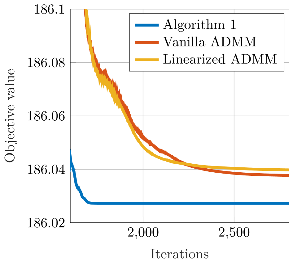
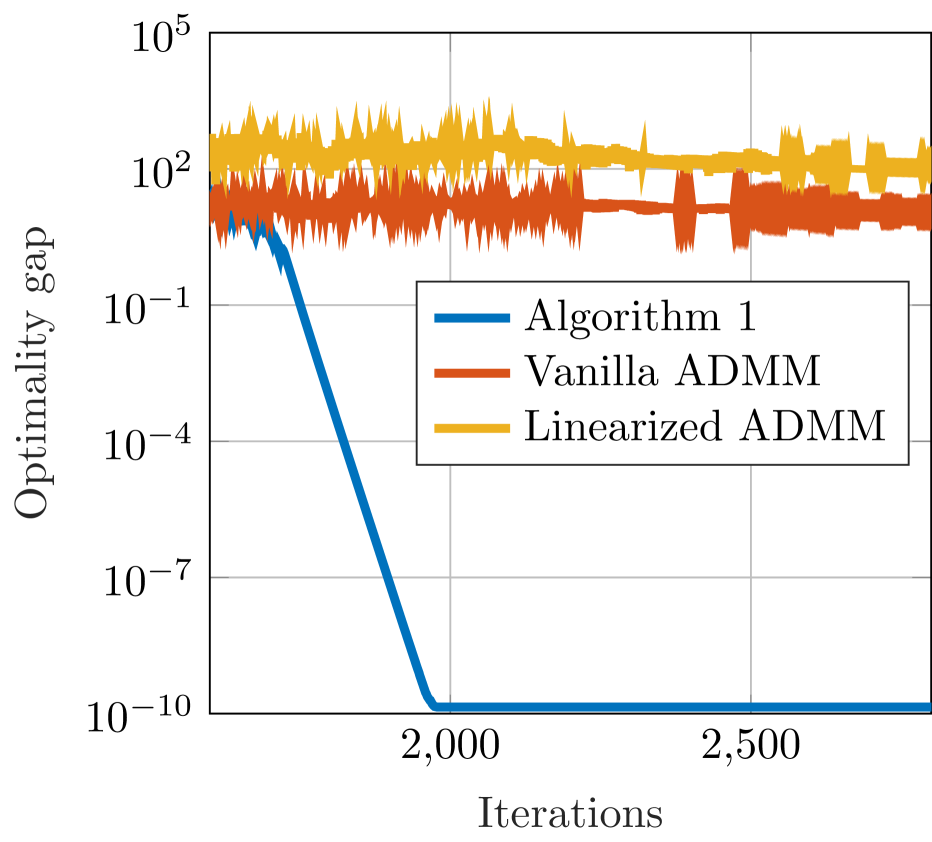
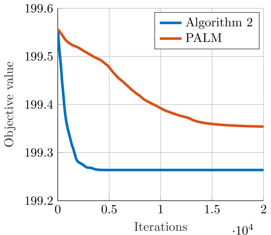
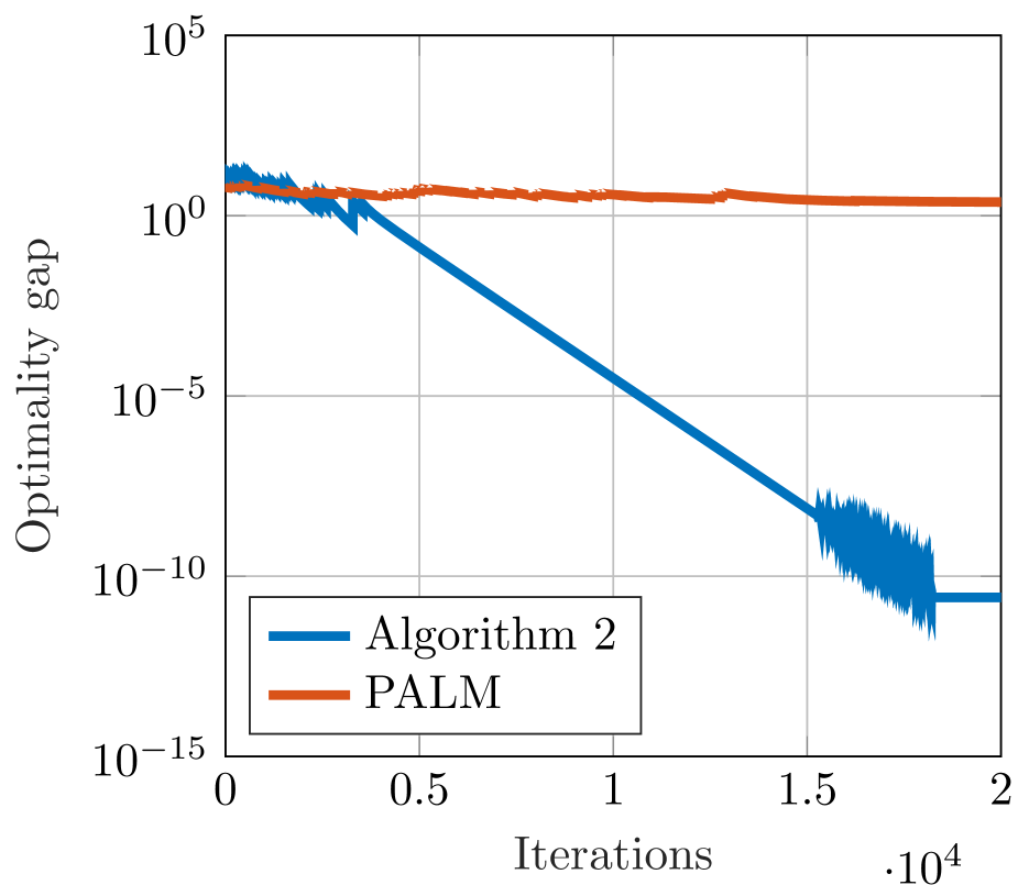
Figure 2: Experimental comparison on robust regression. Upper row: Comparison of primal-dual type methods (linearized ADMM [5, 15], vanilla ADMM [7] and Algorithm 1). Lower row: Comparison of primal methods (PALM [4] and Algorithm 2). It is observed that our algorithms converge to critical points of (1) with low objective value. Both ADMM and PALM fail to converge to a critical point of (1).

Table 1: Comparison of linearized ADMM [5, 15], and Algorithm 1 on joint feature selection and semi-supervised learning. The results are consistent with the previous experiment. Note that for the supervised case, due to the convexity and smoothness of $e_{\lambda}f$, linearized ADMM and our algorithm converge to the same solution.

	linearized ADMM					Algorithm 1
$\nicefrac{{l}}{{N}}$	Test Error	Objective	$\nicefrac{{\|u\|_{0}}}{{d}}$	Iterations	Gap	Test Error	Objective	$\nicefrac{{\|u\|_{0}}}{{d}}$	Iterations	Gap
0.10 %	1.00 %	138.62	1.00 %	60000	12	0.95 %	$\mathbf{107.38}$	0.60 %	54518	$\mathbf{1.2\cdot 10^{-5}}$
0.50 %	1.00 %	138.29	0.40 %	60000	10	0.97 %	$\mathbf{109.27}$	0.40 %	49880	$\mathbf{1.1\cdot 10^{-5}}$
5.00 %	1.05 %	132.57	2.59 %	60000	10	1.02 %	$\mathbf{105.80}$	2.79 %	50313	$\mathbf{1.3\cdot 10^{-5}}$
7.00 %	1.10 %	127.23	3.59 %	60000	9.5	1.12 %	$\mathbf{101.10}$	2.99 %	54876	$\mathbf{1.2\cdot 10^{-5}}$
9.00 %	1.05 %	127.52	4.38 %	60000	9.3	1.12 %	$\mathbf{101.14}$	3.98 %	53439	$\mathbf{1.2\cdot 10^{-5}}$
10.00 %	1.12 %	128.95	4.38 %	60000	8.9	1.07 %	$\mathbf{103.72}$	3.98 %	49452	$\mathbf{1.1\cdot 10^{-5}}$
100.00 %	1.40 %	$\mathbf{116.34}$	47.61 %	56815	$\mathbf{1.5\cdot 10^{-5}}$	1.40 %	$\mathbf{116.34}$	47.61 %	56815	$\mathbf{1.5\cdot 10^{-5}}$

5.1 Robust Linear Regression

In linear regression one is interested in reconstructing a signal $u\in\mathbb{R}^{n}$ from noisy measurements $b\in\mathbb{R}^{m}$. The forward model takes the form of

$$b=Au+\epsilon,$$

where $A\in\mathbb{R}^{m\times n}$ describes the linear sampling and $\epsilon\in\mathbb{R}^{m}$ is a disturbance term.

Instead of plain least squares, we use the truncated quadratic loss $e_{\lambda}f_{i}(v_{i})=\min\,\{\nu,\frac{1}{2\lambda}v_{i}^{2}\}$, which is more robust against outliers [23, 16]. We set $g(u)=0$ and the data term $e_{\lambda}f(v)=\sum_{i=1}^{n}e_{\lambda}f_{i}(v_{i})$ with $f_{i}(v):=\nu\|v_{i}\|_{0}$ chosen as the $\ell_{0}$-norm.

We benchmark linearized ADMM [5, 15], vanilla ADMM [7], PALM [4] and Algorithms 1 and 2 on synthetic data. The entries of $A\in\mathbb{R}^{20000\times 10}$ and $b\in\mathbb{R}^{20000}$ are i.i.d. and normal distributed. We further degrade $b$ with additive Gaussian and high impulsive noise by adding a large constant to $60\%$ of the entries. We manually choose $\lambda=0.05$ and $\nu=0.01$. For both ADMM and our proposed Algorithm 1, a warmup phase is launched, where the parameter $\rho$ is initialized with a small value and then grows exponentially along iterations up to a value slightly bigger than $\nicefrac{{1}}{{\lambda}}=20$. In practice, such configuration often leads to lower objective values. To enforce convergence of vanilla and linearized ADMM, we keep increasing $\rho$ until $\rho=8000\gg 20$. Yet, as shown in Figure 2, both ADMM and PALM fail to converge to a critical point of (1) evidenced by a non-vanishing optimality gap. In contrast, our Algorithm finds critical points with lower objective values.

5.2 Joint Semi-supervised Learning and Feature Selection

To further demonstrate versatility of our model, we consider the problem of joint feature selection [3] and semi-supervised learning with linear classifiers. We use a Huberized semi-supervised SVM model [2, 12, 6] and a nonconvex, sparsity-promoting regularizer on the classifier. The overall task is to learn a classifier from both labeled and unlabeled examples and, simultaneously, select the features.

We set up the individual components of model (1) as follows. Let $N$ be the number of training examples, among which $l\leq N$ examples are labeled and the rest is unlabeled. Let $X\in\mathbb{R}^{N\times d}$ be the feature matrix and $u\in\mathbb{R}^{d}$ the linear classifier. We introduce a linear constraint $Xu=v$. We model the term $e_{\lambda}f$ as the sum of two terms: the first corresponds to the $N-l$ unlabeled training examples; the second term corresponds to the the labeled examples. More explicitly, the data term reads

$$e_{\lambda}f(v)=\sum_{i=1}^{N-l}e_{\lambda}f_{i}(v_{i})+\sum_{j=N-l+1}^{N}e_{\lambda}f_{j}(v_{j}).$$

For $i\leq N-l$ and $f_{i}(v_{i})=\min_{\theta_{i}\in\{-1,1\}}(1-v_{i}\theta_{i})_{+}$, each summand $e_{\lambda}f_{i}(v_{i})$ is a “symmetric Huberized hinge loss” term, whose shape is depicted in Figure 1. For $j>N-l$, the label $\theta_{j}\in\{-1,1\}$ is fixed and $e_{\lambda}f_{j}(v_{j})$ is the plain Huberized hinge loss for $f_{j}(v_{j})=(1-v_{j}\theta_{j})_{+}$.

For feature selection, we promote sparsity on the classifier $u$ by the $\ell_{0}$-norm regularization. We also include a squared $\ell_{2}$ norm, $\beta\|u\|^{2}$, to control the margin in the SVM model and ensure the coercivity of the model. Altogether, the regularization term $g$ is set up as $g(u)=\alpha\|u\|_{0}+\beta\|u\|^{2}$. To avoid extremal solutions, we fix the bias in the SVM model to the empirical mean of the data, which amounts to solving the $\mathit{NP}$-hard Furthest Hyperplane Problem (FHP) [13].

In Table 1 we benchmark linearized ADMM [5, 15] vs. Algorithm 1 on synthetic data ($N=12000$ examples) that is not linearly separable and degraded by $d=500$ additional feature components containing noise. We manually choose $\alpha=0.025$, $\beta=0.416$, $\lambda=0.5$. We stop the algorithm, when the difference of consecutive iterates is below a threshold $\epsilon=10^{-7}$ or the maximum number of $60000$ iterations is reached. The results are consistent with the previous example: Linearized ADMM does not converge to a critical point within the maximum number of iterations, except for the supervised case $l=N$. In this case, Algorithm 1 and linearized ADMM converge to the same result, due to the convexity of $f$ resp. smoothness of $e_{\lambda}f$.

6 Conclusion

In this work we have tackled highly nonconvex Moreau-Yosida regularized composite problems, where both terms in the objective are nonsmooth. Classical proximal splitting algorithms such as nonconvex ADMM fail to converge for this problem class. To overcome this limitation, we devised a novel primal-dual proximal splitting algorithm that intrinsically regularizes the behavior of the dual variable. For piecewise convex functions, we derived explicit qualification conditions that guarantee convergence to a critical point of the Moreau-Yosida regularized problem. We validated our method on the optimization of challenging highly nonconvex machine learning objectives. For future work we will address a randomized variant of our algorithm suited to distributed computation in large-scale machine learning.

Acknowledgements

We would like to thank Matthias Vestner and Thomas Möllenhoff for fruitful discussions and helpful comments. We gratefully acknowledge the support of the ERC Consolidator Grant 3D Reloaded.

Appendix A Proofs

A.1 Proof of Lemma 1

Proof.

(Statements 1 & 2) To show the lower boundedness of $\mathfrak{Q}_{\rho}(u^{t+1},z^{t+1},y^{t+1})$ we rewrite

$$\mathfrak{Q}_{\rho}(u^{t+1},z^{t+1},y^{t+1})=f(z^{t+1})+g(u^{t+1})$$

$$\qquad+\frac{\rho}{2}\|Au^{t+1}-z^{t+1}-\lambda y^{t+1}\|^{2}$$

$$\qquad+\frac{1}{2\lambda}\|Au^{t+1}-z^{t+1}\|^{2}$$

$$\qquad-\frac{1}{2\lambda}\|Au^{t+1}-z^{t+1}-\lambda y^{t+1}\|^{2}.$$

Since $\rho>\frac{1}{\lambda}$ we can further bound $\mathfrak{Q}_{\rho}(u^{t+1},z^{t+1},y^{t+1})$ from below by the quadratic penalty $Q(u^{t+1},z^{t+1})$ in (7):

$$\mathfrak{Q}_{\rho}(u^{t+1},z^{t+1},y^{t+1})\geq Q(u^{t+1},z^{t+1}).$$

We further bound $Q(u^{t+1},z^{t+1})$:

$$Q(u^{t+1},z^{t+1}) \geq e_{\lambda}f(Au^{t+1})+g(u^{t+1}),$$

which is bounded from below.
(Statement 3) We find an estimate for $\mathfrak{Q}_{\rho}(u^{t+1},z^{t},y^{t})-\mathfrak{Q}_{\rho}(u^{t},z^{t},y^{t})$. By the definition of $u^{t+1}$ as the global minimum of $\mathfrak{Q}_{\rho}(\cdot,z^{t},y^{t})+\frac{1}{2}\|(\cdot)-u^{t}\|_{M}^{2}$ and $M:=\frac{1}{\sigma}I-\rho A^{\top}A$ positive definite for $\sigma\rho\|A\|^{2}<1$, we have the estimate

$$\mathfrak{Q}_{\rho}(u^{t+1},z^{t},y^{t})+\frac{1}{2}\|u^{t+1}-u^{t}\|_{M}^{2}\leq\mathfrak{Q}_{\rho}(u^{t},z^{t},y^{t}).$$

We bound $\frac{1}{2}\|u^{t+1}-u^{t}\|_{M}^{2}$,

$$\|u^{t+1}-u^{t}\|_{M}^{2} =\langle u^{t+1}-u^{t},M(u^{t+1}-u^{t})\rangle$$

$$=\frac{1}{\sigma}\|u^{t+1}-u^{t}\|^{2}-\rho\|Au^{t+1}-Au^{t}\|^{2}$$

$$\geq\left(\frac{1}{\sigma}-\rho\|A\|^{2}\right)\|u^{t+1}-u^{t}\|^{2}.$$

This yields the estimate

$$\mathfrak{Q}_{\rho}(u^{t+1},z^{t},y^{t})-\mathfrak{Q}_{\rho}(u^{t},z^{t},y^{t})$$ (20)

$$\qquad\leq\left(\frac{\rho\|A\|^{2}}{2}-\frac{1}{2\sigma}\right)\|u^{t+1}-u^{t}\|^{2},$$

which leads to a sufficient descent if $\sigma\rho\|A\|^{2}<1$. The optimality for the $z$-update guarantees

$$\mathfrak{Q}_{\rho}(u^{t+1},z^{t+1},y^{t})-\mathfrak{Q}_{\rho}(u^{t+1},z^{t},y^{t})\leq 0.$$ (21)

Finally we bound the term

$$\mathfrak{Q}_{\rho}(u^{t+1},z^{t+1},y^{t+1})-\mathfrak{Q}_{\rho}(u^{t+1},z^{t+1},y^{t})=-\frac{\lambda}{2}\|y^{t+1}\|^{2}$$

$$\qquad+\frac{\lambda}{2}\|y^{t}\|^{2}+\langle Au^{t+1}-z^{t+1},y^{t+1}-y^{t}\rangle$$

$$\qquad+\frac{\rho}{2}\|Au^{t+1}-z^{t+1}-\lambda y^{t+1}\|^{2}$$

$$\qquad-\frac{\rho}{2}\|Au^{t+1}-z^{t+1}-\lambda y^{t}\|^{2}.$$

Since $\frac{1}{\rho}(y^{t+1}-y^{t})+\lambda y^{t+1}=Au^{t+1}-z^{t+1}$, we can rewrite

$$-\frac{\lambda}{2}\|y^{t+1}\|^{2}+\frac{\lambda}{2}\|y^{t}\|^{2}+\langle Au^{t+1}-z^{t+1},y^{t+1}-y^{t}\rangle$$

$$=-\frac{\lambda}{2}\|y^{t+1}\|^{2}+\frac{\lambda}{2}\|y^{t}\|^{2}+\frac{1}{\rho}\|y^{t+1}-y^{t}\|^{2}+\lambda\|y^{t+1}\|^{2}$$

$$\qquad-\lambda\langle y^{t+1},y^{t}\rangle$$

$$=\frac{\lambda}{2}\|y^{t+1}\|^{2}-\lambda\langle y^{t+1},y^{t}\rangle+\frac{\lambda}{2}\|y^{t}\|^{2}+\frac{1}{\rho}\|y^{t+1}-y^{t}\|^{2}$$

$$=\left(\frac{1}{\rho}+\frac{\lambda}{2}\right)\|y^{t+1}-y^{t}\|^{2}.$$

We apply the identity $\|a+c\|^{2}-\|b+c\|^{2}=-\|b-a\|^{2}+2\langle a+c,a-b\rangle$ with $a:=-\lambda y^{t+1}$, $b:=-\lambda y^{t}$ and $c:=Au^{t+1}-z^{t+1}$ and obtain

$$\frac{\rho}{2}\|Au^{t+1}-z^{t+1}-\lambda y^{t+1}\|^{2}-\frac{\rho}{2}\|Au^{t+1}-z^{t+1}-\lambda y^{t}\|^{2}$$

$$=-\frac{\rho\lambda^{2}}{2}\|y^{t+1}-y^{t}\|^{2}$$

$$\qquad-\lambda\rho\langle Au^{t+1}-z^{t+1}-\lambda y^{t+1},y^{t+1}-y^{t}\rangle$$

$$=-\frac{\rho\lambda^{2}+2\lambda}{2}\|y^{t+1}-y^{t}\|^{2}.$$

Overall we have:

$$\mathfrak{Q}_{\rho}(u^{t+1},z^{t+1},y^{t+1})-\mathfrak{Q}_{\rho}(u^{t+1},z^{t+1},y^{t})$$ (22)

$$\qquad=\left(\frac{1}{\rho}-\frac{\rho\lambda^{2}+\lambda}{2}\right)\|y^{t+1}-y^{t}\|^{2}.$$

Summing (20)–(22), we obtain the desired result:

$$\mathcal{Q}_{\rho}(u^{t+1},z^{t+1},y^{t+1})-\mathcal{Q}_{\rho}(u^{t},z^{t},y^{t})$$ (23)

$$\quad\leq\left(\frac{\rho\|A\|^{2}}{2}-\frac{1}{2\sigma}\right)\|u^{t+1}-u^{t}\|^{2}$$

$$\quad\quad+\left(\frac{1}{\rho}-\frac{\rho\lambda^{2}+\lambda}{2}\right)\|y^{t+1}-y^{t}\|^{2}.$$

∎

A.2 Proof of Lemma 2

Proof.

Since $\{\mathfrak{Q}_{\rho}(u^{t},z^{t},y^{t})\}_{t\in\mathbb{N}}$ monotonically decreases by Lemma 1, it is bounded from above. Since $\{Q(u^{t},z^{t})\}_{t\in\mathbb{N}}$ is bounded from above by $\{\mathfrak{Q}_{\rho}(u^{t},z^{t},y^{t})\}_{t\in\mathbb{N}}$ and, furthermore, $Q$ is coercive by assumption, we assert that $\{u^{t}\}_{t\in\mathbb{N}}$, $\{z^{t}\}_{t\in\mathbb{N}}$ are uniformly bounded.

Now we sum the estimate (23) from $t=1$ to $T$ and obtain due to the lower boundedness of the iterates $\mathfrak{Q}_{\rho}(u^{t},z^{t},y^{t})$:

$$-\infty <\mathfrak{Q}_{\rho}(u^{T+1},z^{T+1},y^{T+1})-\mathfrak{Q}_{\rho}(u^{1},z^{1},y^{1})$$

$$\leq\left(\frac{\rho\|A\|^{2}}{2}-\frac{1}{2\sigma}\right)\sum_{t=1}^{T}\|u^{t+1}-u^{t}\|^{2}$$

$$\quad+\left(\frac{1}{\rho}-\frac{\rho\lambda^{2}+\lambda}{2}\right)\sum_{t=1}^{T}\|y^{t+1}-y^{t}\|^{2}.$$

Passing $T\to\infty$ yields that $\|u^{t+1}-u^{t}\|\to 0$ and $\|y^{t+1}-y^{t}\|\to 0$ for $\rho>\nicefrac{{1}}{{\lambda}}$ and $\sigma\rho\|A\|^{2}<1$. From $\frac{1}{\rho}(y^{t+1}-y^{t})=Au^{t+1}-z^{t+1}-\lambda y^{t+1}$ we have that,

$$0 \leq\|z^{t}-z^{t+1}\|$$

$$=\|z^{t}-z^{t+1}+A(u^{t+1}-u^{t})-A(u^{t+1}-u^{t})$$

$$\qquad+\lambda y^{t+1}-\lambda y^{t}-\lambda y^{t+1}+\lambda y^{t}\|$$

$$\leq\frac{1}{\rho}\|y^{t+1}-y^{t}\|+\|A\|\|u^{t+1}-u^{t}\|$$

$$\qquad+\lambda\|y^{t+1}-y^{t}\|\to 0,$$

and that $\|Au^{t}-z^{t}-\lambda y^{t}\|\to 0$. Since $\{u^{t}\}_{t\in\mathbb{N}}$, $\{z^{t}\}_{t\in\mathbb{N}}$ are uniformly bounded, also $\{y^{t}\}_{t\in\mathbb{N}}$ are uniformly bounded. ∎

References

- [1] Marco Artina, Massimo Fornasier, and Francesco Solombrino. Linearly constrained nonsmooth and nonconvex minimization. SIAM Journal on Optimization, 23(3):1904–1937, 2013.
- [2] Kristin P Bennett and Ayhan Demiriz. Semi-supervised support vector machines. In Advances in Neural Information Processing Systems (NIPS), pages 368–374, 1999.
- [3] Jinbo Bi, Kristin Bennett, Mark Embrechts, Curt Breneman, and Minghu Song. Dimensionality reduction via sparse support vector machines. Journal of Machine Learning Research, 3:1229–1243, 2003.
- [4] Jérôme Bolte, Shoham Sabach, and Marc Teboulle. Proximal alternating linearized minimization for nonconvex and nonsmooth problems. Mathematical Programming, 146(1-2):459–494, 2014.
- [5] Antonin Chambolle and Thomas Pock. A first-order primal-dual algorithm for convex problems with applications to imaging. Journal of Mathematical Imaging and Vision, 40(1):120–145, 2011.
- [6] Ronan Collobert, Fabian Sinz, Jason Weston, and Léon Bottou. Large scale transductive SVMs. Journal of Machine Learning Research, 7:1687–1712, 2006.
- [7] Jonathan Eckstein and Dimitri P. Bertsekas. On the Douglas-Rachford splitting method and the proximal point algorithm for maximal monotone operators. Mathematical Programming, 55:293–318, 1992.
- [8] Daniel Gabay. Applications of the method of multipliers to variational inequalities. Studies in Mathematics and Its Applications, 15:299–331, 1983.
- [9] Daniel Gabay and Bertrand Mercier. A dual algorithm for the solution of nonlinear variational problems via finite element approximation. Computers & Mathematics with Applications, 2(1):17–40, 1976.
- [10] Roland Glowinski and Americo Marrocco. Sur l’approximation, par éléments finis d’ordre un, et la résolution, par pénalisation-dualité d’une classe de problèmes de Dirichlet non linéaires. Revue Française d’Automatique, Informatique, Recherche Opérationnelle. Analyse Numérique, 9(2):41–76, 1975.
- [11] Mingyi Hong, Zhi-Quan Luo, and Meisam Razaviyayn. Convergence analysis of alternating direction method of multipliers for a family of nonconvex problems. SIAM Journal on Optimization, 26(1):337–364, 2016.
- [12] Thorsten Joachims. Transductive inference for text classification using support vector machines. In Proceedings of the 16th International Conference on Machine Learning (ICML 1999), pages 200–209, 1999.
- [13] Zohar Karnin, Edo Liberty, Shachar Lovett, Roy Schwartz, and Omri Weinstein. Unsupervised SVMs: On the complexity of the furthest hyperplane problem. In Conference on Learning Theory, pages 2–1, 2012.
- [14] Guoyin Li and Ting Kei Pong. Global convergence of splitting methods for nonconvex composite optimization. SIAM Journal on Optimization, 25(4):2434–2460, 2015.
- [15] Zhouchen Lin, Risheng Liu, and Zhixun Su. Linearized alternating direction method with adaptive penalty for low-rank representation. In Advances in Neural Information Processing Systems (NIPS), pages 612–620, 2011.
- [16] Tzu-Ying Liu and Hui Jiang. Minimizing sum of truncated convex functions and its applications. Journal of Computational and Graphical Statistics, 2017.
- [17] Thomas Möllenhoff, Evgeny Strekalovskiy, Michael Moeller, and Daniel Cremers. The primal-dual hybrid gradient method for semiconvex splittings. SIAM Journal on Imaging Sciences, 8(2):827–857, 2015.
- [18] Jean-Jacques Moreau. Proximité et dualité dans un espace Hilbertien. Bull. Soc. Math. France, 93(2):273–299, 1965.
- [19] Yurii Nesterov. Gradient methods for minimizing composite functions. Mathematical Programming, 140(1):125–161, 2013.
- [20] Peter Ochs. Local convergence of the heavy-ball method and iPiano for non-convex optimization. arXiv preprint arXiv:1606.09070, 2016.
- [21] Peter Ochs, Yunjin Chen, Thomas Brox, and Thomas Pock. iPiano: Inertial proximal algorithm for nonconvex optimization. SIAM Journal on Imaging Sciences, 7(2):1388–1419, 2014.
- [22] R. Tyrrell Rockafellar and Roger J.-B. Wets. Variational Analysis. Springer, 1998.
- [23] Yiyuan She and Art B Owen. Outlier detection using nonconvex penalized regression. Journal of the American Statistical Association, 106(494):626–639, 2011.
- [24] Yu Wang, Wotao Yin, and Jinshan Zeng. Global convergence of ADMM in nonconvex nonsmooth optimization. arXiv:1511.06324v5, 2017.