Finite continuum quasi distributions from lattice QCD

Abstract

We present a new approach to extracting continuum quasi distributions from lattice QCD. Quasi distributions are defined by matrix elements of a Wilson-line operator extended in a spatial direction, evaluated between nucleon states at finite momentum. We propose smearing this extended operator with the gradient flow to render the corresponding matrix elements finite in the continuum limit. This procedure provides a nonperturbative method to remove the power-divergence associated with the Wilson line and the resulting matrix elements can be directly matched to light-front distributions via perturbation theory.

1 Introduction

Protons and neutrons—nucleons—are the basic, observable building blocks of the visible matter in the Universe. But nucleons are not simple building blocks: they are strongly-coupled, dynamical systems, composed of quarks and gluons bound together by the strong nuclear force. Quantum chromodynamics (QCD) is the gauge theory of the strong nuclear force that, in principle, connects protons and neutrons to their constituent quarks and gluons. In practice, however, piecing together nucleon structure directly from QCD has proved challenging, largely due to the nonperturbative nature of QCD at energy scales around the nucleon mass.

Parton distribution functions (PDFs), which characterise the distribution of a fast-moving nucleon’s longitudinal momentum amongst its constituents, have posed particular difficulties for first principles’ QCD calculations. PDFs are most naturally formulated as matrix elements of null-separated quark fields, which cannot be calculated using Euclidean lattice QCD, the only ab initio, systematically-improvable method currently available for nonperturbative QCD calculations. In Ji:2013dva , Ji proposed a promising method to extract PDFs, from lattice QCD calculations of quasi distributions, which are spatially-extended operators between nucleon states at finite momentum. Related frameworks have also been proposed: in Ma:2014jla ; Ma:2014jga ; Ma:2017pxb quasi distributions were treated as “lattice cross-sections” from which light-front PDFs can be factorized and Refs. Radyushkin:2016hsy ; Orginos:2017kos introduced and studied the closely-related pseudo distributions.

Quasi and pseudo distributions are matrix elements of time-local operators that can be computed using lattice QCD Carlson:2017gpk ; Briceno:2017cpo and preliminary nonperturbative results are encouraging Lin:2014zya ; Alexandrou:2015rja ; Chen:2016utp ; Orginos:2017kos ; Zhang:2017bzy ; Alexandrou:2017qpu . Moreover, a number of theoretical issues Li:2016amo ; Carlson:2017gpk ; Rossi:2017muf have now been clarified: the multiplicative renormalisation of the spatial Wilson line operator has been proven Ji:2017oey ; Ishikawa:2017faj ; the factorization of light-front PDFs from quasi distributions was demonstrated in Ma:2014jla ; Ma:2014jga ; and a proof that the matrix element extracted from Euclidean correlation functions is identical to that determined from a Lehmann-Symanzik-Zimmermann reduction procedure in Minkowski spacetime provided in Briceno:2017cpo and studied further in Xiong:2017jtn ; Ji:2017rah .

On the lattice, there is a power-divergence, which scales exponentially with the length of the Wilson line divided by the lattice spacing, associated with the extended operator that defines quasi and pseudo distributions. Several approaches have been proposed: inspired by heavy quark effective theory, the authors of Chen:2016fxx ; Ishikawa:2016znu suggested an exponentiated mass renormalisation to remove the power-divergence and, more recently, RI/MOM Chen:2017mzz ; Stewart:2017tvs and RI^′ Alexandrou:2017huk schemes have been introduced. In Monahan:2016bvm , we presented an alternative approach, the smeared quasi distribution, that avoids some of the challenges of the power divergence by taking advantage of the properties of the gradient flow Narayanan:2006rf ; Luscher:2011bx ; Luscher:2013cpa .

The gradient flow exponentially suppresses ultraviolet (UV) field fluctuations, which corresponds to smearing out the original degrees of freedom in real space. Most importantly, the gradient flow renders correlation functions finite Luscher:2011bx , up to a multiplicative fermion wavefunction renormalisation Luscher:2013cpa and provided one has fixed the renormalised parameters of the original theory. Fixing the flow time, which corresponds to a real-space smearing scale, in physical units, ensures that matrix elements determined at finite lattice spacing remain finite in the continuum limit. The gradient flow therefore enables us to extract finite quasi distributions from lattice calculations Monahan:2016bvm . The resulting continuum matrix element can be directly matched to the light-front PDF, or to the quasi distribution renormalised in, for example, the $\overline{MS}$ scheme Xiong:2013bka ; Ji:2015jwa ; Constantinou:2017sej ; Wang:2017qyg .

Here we introduce smeared quasi distributions and study the corresponding matrix element at one loop in perturbation theory. We compute the matrix element of the smeared Wilson-line operator between external, gauge-fixed quark states. As we demonstrate, the Wilson-line power divergence appears at one loop as a contribution linear in $\overline{z}=z/r_{\tau}$, where $z$ is the length of the Wilson line and $r_{\tau}$ is the gradient flow smearing radius, for $\overline{z}\gg 1$. Subtracting this contribution, the remaining matrix element is finite, and has a well-defined $\overline{z}\to 0$ limit, in contrast to the $\overline{MS}$ scheme. In the small flow-time regime, $\overline{z}\gg 1$, the matrix element depends only logarithmically on $\overline{z}$ and thus satisfies a relation similar to a standard renormalisation group equation.

2 Light-front and quasi distributions

We consider only flavour nonsinglet unpolarised quasi and light-front PDFs, for which we can ignore mixing with the gluon distribution. Extending our discussion to the polarised distribution is straightforward.

2.1 Light-front PDFs

We write the renormalised light-front PDFs as $f(\xi,\mu)$, where we have introduced light-front coordinates $x^{\pm}=(t\pm z)/\sqrt{2}$, a renormalisation scale $\mu$, and $\xi=k^{+}/P^{+}$. In general, we can relate the renormalised light-front PDFs to the bare PDFs, $f^{(0)}(\xi)$, through

$$f(\xi,\mu)=\int_{\xi}^{1}\frac{\mathrm{d}\zeta}{\zeta}{\cal Z}\left(\frac{\xi}{\zeta},\mu\right)f^{(0)}(\zeta),$$ (1)

where the bare PDF is given by Collins:2011zzd

$$f^{(0)}(\xi)=\int_{-\infty}^{\infty}\frac{\mathrm{d}\omega^{-}}{4\pi}e^{-i\xi P^{+}\omega^{-}}\left\langle P\left|T\,\overline{\psi}(0,\omega^{-},\mathbf{0}_{\mathrm{T}})W(\omega^{-},0)\gamma^{+}\frac{\lambda^{a}}{2}\psi(0)\right|P\right\rangle_{\mathrm{C}}.$$ (2)

Here $T$ indicates time-ordering, $\psi$ is a quark field, and we include only connected contributions, represented by the subscript $C$. The Wilson line operator is

$$W(\omega^{-},0)={\cal P}\exp\left[-ig_{0}\int_{0}^{\omega^{-}}\mathrm{d}y^{-}A^{+}_{a}(0,y^{-},\mathbf{0}_{\mathrm{T}})T_{a}\right],$$ (3)

where ${\cal P}$ is the path-ordering operator, $g_{0}$ the QCD bare coupling, and $A_{\alpha}=A_{\alpha}^{a}T^{a}$ is the $SU(3)$ gauge potential with generator $T^{a}$ (summation over the color index $a$ implicit). The nucleon state, $|P\rangle$, is a spin-averaged, exact momentum eigenstate with relativistic normalisation

$$\langle P^{\prime}|P\rangle=(2\pi)^{3}2P^{+}\delta\left(P^{+}-P^{\prime\,+}\right)\delta^{(2)}\left(\mathbf{P}_{\mathrm{T}}-\mathbf{P}^{\prime}_{\mathrm{T}}\right).$$ (4)

The renormalised nonsinglet PDFs satisfy a DGLAP equation Gribov:1972rt ; Dokshitzer:1977sg ; Altarelli:1977zs that describes their scale dependence

$$\mu\frac{\mathrm{d}\,f(x,\mu)}{\mathrm{d}\mu}=\frac{\alpha_{s}(\mu)}{\pi}\bigintsss_{x}^{1}\frac{\mathrm{d}y}{y}f(y,\mu)P\left(\frac{x}{y}\right),$$ (5)

were $P\left(z\right)$ is a function whose moments are given by

$$\int_{0}^{1}\mathrm{d}x\,x^{n-1}P(x)=\gamma^{(n)}.$$ (6)

The anomalous dimensions, $\gamma^{(n)}$, satisfy

$$\left[\mu\frac{\mathrm{d}\;}{\mathrm{d}\mu}-\frac{\alpha_{s}(\mu)}{\pi}\gamma^{(n)}\right]a^{(n)}(\mu)=0.$$ (7)

Here $\alpha_{s}(\mu)$ is the (renormalised) strong coupling constant and the $a^{(n)}(\mu)$ are the renormalised Mellin moments of the PDF,

$$a^{(n)}(\mu)=\int_{0}^{1}\mathrm{d}\xi\,\xi^{n-1}\left[f(\xi,\mu)+(-1)^{n}\overline{f}(\xi,\mu)\right]=\int_{-1}^{1}\mathrm{d}\xi\,\xi^{n-1}f(\xi,\mu),$$ (8)

which are related to matrix elements of renormalised twist-two operators, ${\cal O}^{\{\nu_{1}\ldots\nu_{n}\}}(\mu)=Z_{\cal O}(\mu){\cal O}_{0}^{\{\nu_{1}\ldots\nu_{n}\}}$, through

$$\left\langle P|{\cal O}^{\{\nu_{1}\ldots\nu_{n}\}}(\mu)|P\right\rangle=2a^{(n)}(\mu)\left(P^{\nu_{1}}\cdots P^{\nu_{n}}-\mathrm{traces}\right).$$ (9)

2.2 Smeared quasi distributions

In Monahan:2016bvm , we proposed a new approach to extracting continuum quasi distributions from lattice calculations, constructing finite matrix elements by smearing both the fermion and gauge fields via the gradient flow Narayanan:2006rf ; Luscher:2011bx ; Luscher:2013cpa . Further details of the gradient flow, and a variety of applications in lattice calculations, are given in the reviews Luscher:2013vga ; Ramos:2015dla .

We use ringed fermion fields at flow time $\tau$ Makino:2014taa ; Hieda:2016lly , denoted by $\overline{\chi}(x;\tau)$ and $\chi(x;\tau)$, and construct a smeared Wilson line operator, ${\bf\cal W}(x_{1},x_{2};\tau)$, from smeared gauge fields $B_{\alpha}(x;\tau)$. We then define the connected matrix element

$$h_{\alpha}^{(s)}\left(\frac{n^{2}}{\tau},n\cdot P,\sqrt{\tau}\Lambda_{\mathrm{QCD}},\sqrt{\tau}M_{\mathrm{N}}\right)=\frac{1}{2P_{z}}\left\langle P_{z}\left|\overline{\chi}(n;\tau){\bf\cal W}(0,n;\tau)\gamma_{\alpha}\frac{\lambda^{a}}{2}\chi(0;\tau)\right|P_{z}\right\rangle_{\mathrm{C}},$$ (10)

which depends only on dimensionless combinations of scales and Euclidean SO(4) invariants Radyushkin:2016hsy . The spacetime position of the antiquark field, $n=(\mathbf{0},z,0)$, is a four-vector usually chosen to be in the $z$-direction. Ringed fermion fields require no wavefunction renormalisation and this smeared matrix element remains finite provided the flow time, $\tau>0$, is fixed in physical units, because correlation functions constructed from smeared fields are finite Luscher:2011bx ; Luscher:2013cpa . As we illustrate later at one loop in perturbation theory, divergences appear in the limit of vanishing flow time and the matrix element requires renormalisation in this limit. The Lorentz index $\alpha$ is arbitrary, although choosing $\alpha=4$ simplifies lattice calculations by removing mixing at finite lattice spacing Constantinou:2017sej and eliminating some higher-twist contamination Radyushkin:2016hsy .

We define the smeared quasi distribution Monahan:2016bvm as

$$q^{\,(s)}\left(\xi,\sqrt{\tau}P_{z},\sqrt{\tau}\Lambda_{\mathrm{QCD}},\sqrt{\tau}M_{\mathrm{N}}\right)=\int_{-\infty}^{\infty}\frac{\mathrm{d}z}{2\pi}e^{i\xi zP_{z}}P_{z}h^{(s)}\left(\frac{n^{2}}{\tau},n\cdot P,\sqrt{\tau}\Lambda_{\mathrm{QCD}},\sqrt{\tau}M_{\mathrm{N}}\right),$$ (11)

where $\xi$ is best interpreted as a dimensionless momentum variable in a Fourier transformation. Working in the regime in which

$$\Lambda_{QCD},M_{N}\ll P_{z}\ll\tau^{-1/2},$$ (12)

the smeared quasi distribution can be directly related to the light-front distribution by Monahan:2016bvm

$$q^{\,(s)}\left(x,\sqrt{\tau}\Lambda_{\mathrm{QCD}},\sqrt{\tau}P_{z}\right)=\int_{-1}^{1}\frac{d\xi}{\xi}\,\widetilde{Z}\left(\frac{x}{\xi},\sqrt{\tau}\mu,\sqrt{\tau}P_{z}\right)f(\xi,\mu)+{\cal O}(\sqrt{\tau}\Lambda_{\mathrm{QCD}}).$$ (13)

In analogy to the light-front PDFs, in Monahan:2016bvm we derived a DGLAP-like equation for the matching kernel that relates smeared quasi PDFs and light-front PDFs, given by

$$\mu\frac{d\;}{d\mu}\,\widetilde{Z}\left(x,\sqrt{\tau}\mu,\sqrt{\tau}P_{z}\right)=-\frac{\alpha_{s}(\mu)}{\pi}\bigintsss_{x}^{\infty}\frac{dy}{y}\widetilde{Z}\left(y,\sqrt{\tau}\mu,\sqrt{\tau}P_{z}\right)P\left(\frac{x}{y}\right),$$ (14)

up to corrections of ${\cal O}(\sqrt{\tau}\Lambda_{\mathrm{QCD}})$.

The quasi distribution and the light-front PDF have the same infrared (IR) structure Carlson:2017gpk ; Briceno:2017cpo , so that the matching kernel can be determined in perturbation theory. In this work, we focus on the one-loop renormalisation of the smeared quasi distribution, which can be used to relate the smeared quasi distribution to the quasi distribution at zero flow time. We do not consider the matching between the unsmeared quasi distribution and the light-front PDF, which has been discussed in some detail elsewhere Xiong:2013bka ; Ji:2015jwa .

3 Smeared quasi distributions in perturbation theory

The diagrams in Fig. 1 represent the one-loop contributions to the smeared quasi distribution in generalised Feynman gauge (with $\alpha=\lambda=1$, where $\alpha$ is the standard gauge-fixing parameter and $\lambda$ is a generalised gauge-fixing parameter at nonzero flow time Luscher:2010iy ; Luscher:2011bx ). Axial gauge simplifies the calculation of the quasi distribution, but cannot be consistently generalised to arbitrary flow time.

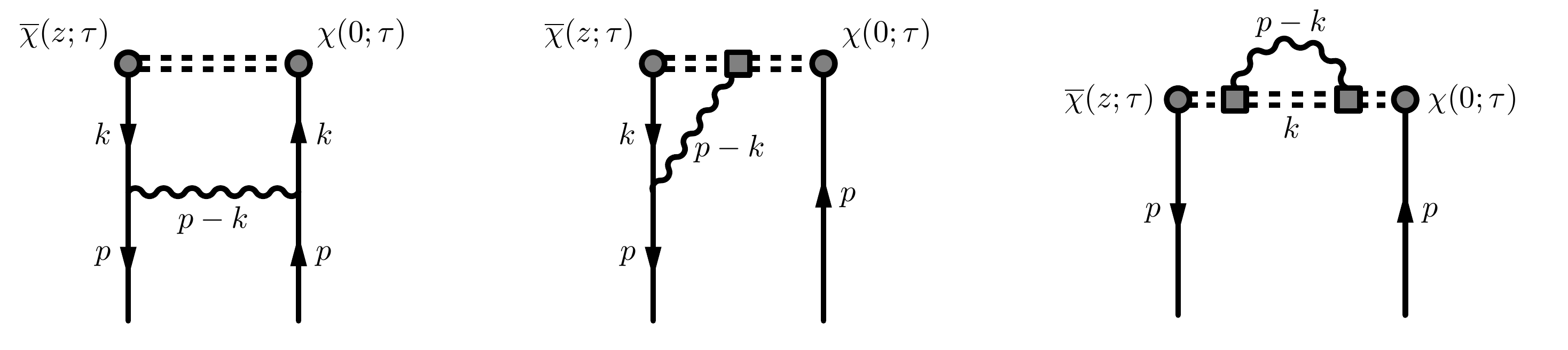
(a)                                     (b)                                     (c)

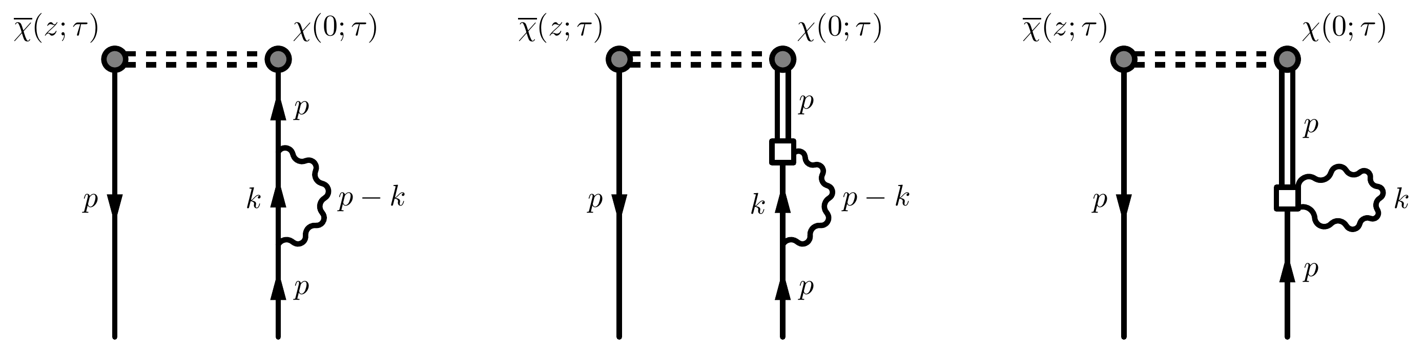
(d)                                     (e)                                     (f)

Figure 1: Diagrams representing the one-loop contributions to the smeared nonsinglet quasi distribution. The grey circles indicate fermion fields at finite flow time $\tau$; solid lines represent fermion propagators; double lines are fermion flow kernels; and open squares are flow vertices at arbitrary flow time $\tau_{1}$.

We analytically determine the renormalisation of one-loop contributions to the matrix element in Eq. (10) by calculating the diagrams in Fig. 1 with external quark states at zero momentum. Some of these contributions have IR divergences, which we regulate with dimensional regularisation. We show that, at one-loop in perturbation theory, these IR divergences are independent of the flow time.

Diagram (d) is the usual wavefunction renormalisation, $Z_{\psi}$, which is independent of the flow time and known well beyond one loop Chetyrkin:1999pq ; we do not consider this diagram any further here. The other contributions are given by Monahan:2017hpu

$$h_{4}^{\mathrm{(a)}}(\overline{z}^{2},\mu^{2}z^{2})={} \left(\frac{g_{0}}{4\pi}\right)^{2}C_{F}\gamma_{4}\bigg{[}\frac{1}{\epsilon_{\mathrm{IR}}}-\gamma_{\mathrm{E}}-\log\left(\pi\mu^{2}z^{2}\right)+1-\frac{1}{\overline{z}^{4}}\Big{(}1-e^{-\overline{z}^{2}}(1+\overline{z}^{2})\Big{)}+\operatorname{Ei}\left(-\overline{z}^{2}\right)\bigg{]},$$ (15)

$$h_{4}^{\mathrm{(b)}}(\overline{z}^{2})={} \left(\frac{g_{0}}{4\pi}\right)^{2}C_{F}\gamma_{4}\cdot 2\bigg{[}1-\gamma_{\mathrm{E}}-\log\left(\overline{z}^{2}\right)+\operatorname{Ei}\left(-\overline{z}^{2}\right)+\frac{1}{\overline{z}^{2}}\left(e^{-\overline{z}^{2}}-1\right)\bigg{]},$$ (16)

$$h_{4}^{\mathrm{(c)}}(\overline{z}^{2})={} \left(\frac{g_{0}}{4\pi}\right)^{2}C_{F}\gamma_{4}\,2\bigg{[}\gamma_{\mathrm{E}}+\log\left(\overline{z}^{2}\right)-\operatorname{Ei}\left(-\overline{z}^{2}\right)-2\left(e^{-\overline{z}^{2}}-1\right)-\sqrt{\pi\overline{z}^{2}}\operatorname{erf}\left(\sqrt{\overline{z}^{2}}\right)\bigg{]},$$ (17)

$$h_{4}^{\mathrm{(e)}}(\mu^{2}\tau)={} \left(\frac{g_{0}}{4\pi}\right)^{2}C_{F}\gamma_{4}\cdot 2\left[\frac{1}{\epsilon_{\mathrm{UV}}}+1+\log\big{(}8\pi\mu^{2}\tau\big{)}\right],$$ (18)

$$h_{4}^{\mathrm{(f)}}(\mu^{2}\tau)={} -\left(\frac{g_{0}}{4\pi}\right)^{2}C_{F}\gamma_{4}\cdot 4\left[\frac{1}{\epsilon_{\mathrm{UV}}}+\frac{1}{2}+\log(8\pi\mu^{2}\tau)\right].$$ (19)

Here $C_{F}=4/3$ is the color factor; $g_{0}$ is the bare coupling; $\operatorname{Ei}\left(z\right)$ is the exponential integral

$$\operatorname{Ei}\left(z\right)=-\int_{-z}^{\infty}\frac{e^{-t}}{t}\mathrm{d}t;$$ (20)

and $\operatorname{erf}\left(z\right)$ is the error function

$$\operatorname{erf}\left(z\right)=\frac{2}{\sqrt{\pi}}\int_{0}^{z}e^{-t^{2}}\mathrm{d}t.$$ (21)

Our results for diagrams (e) and (f), which have UV divergences removed by $Z_{\chi}$, are in agreement with those presented in Endo:2015iea

The complete one-loop smeared matrix element is therefore

$$h_{4}^{(\mathrm{s})}(\overline{z}^{2})={\cal Z}^{(4)}(\overline{z}^{2})h_{4}^{(0)}=Z^{(4)}(\overline{z}^{2},\mu^{2}\tau)Z_{\chi}(\mu^{2}\tau)Z_{\psi}^{-1}h_{4}^{(0)}+{\cal O}(\alpha_{s}^{2}),\quad\mathrm{with}\quad h_{4}^{(0)}=\overline{u}^{s}(p)\frac{\lambda^{a}}{2}\gamma_{4}u^{s}(p)$$ (22)

and

$$Z^{(4)}(\overline{z}^{2},\mu^{2}\tau)=1+\frac{\alpha_{s}(\mu)}{3\pi}\Big{[}h_{4}^{\mathrm{(a)}}(\overline{z}^{2},\mu^{2}\tau)+h_{4}^{\mathrm{(b)}}(\overline{z}^{2})+h_{4}^{\mathrm{(c)}}(\overline{z}^{2})+h_{4}^{\mathrm{(d)}}+h_{4}^{\mathrm{(e)}}(\mu^{2}\tau)+h_{4}^{\mathrm{(f)}}(\mu^{2}\tau)\Big{]}.$$ (23)

The individual nonzero contributions $h^{\mathrm{(i)}}$ are listed in Eqs. (15) to (19). Here $\alpha_{s}(\mu)=g^{2}/(4\pi)$ is the renormalised coupling constant, equal to the bare coupling constant at this order, and is most naturally evaluated at the scale $\mu^{2}=1/(8\tau)$.

3.1 Asymptotic behavior

The small quark-separation limit, $\overline{z}\to 0$, of these results

$$\lim_{\overline{z}\to 0}h_{4}^{(s)}=\left(\frac{g_{0}}{4\pi}\right)^{2}C_{F}\gamma_{\alpha}\left\{\frac{1}{2}-3\left[\frac{1}{\epsilon_{\mathrm{UV}}}+\log\left(8\pi\mu^{2}\tau\right)\right]\right\},$$ (24)

in agreement with the local vector-current result of Hieda:2016lly . Incorporating $Z_{\chi}(\mu^{2}\tau)$ Luscher:2013cpa ; Makino:2014taa , this leads to

$$V_{4}^{(\mathrm{s})}=\lim_{\overline{z}\to 0}h_{4}^{(\mathrm{s})}(\overline{z}^{2})=\bigg{\{}1+\frac{\alpha_{s}}{3\pi}\bigg{[}\frac{1}{2}-\log(432)\bigg{]}\bigg{\}}\overline{\psi}\gamma_{4}\psi.$$ (25)

This local vector-current result is finite, as it must be for a conserved vector current, but nonzero, which is typical for composite operators of ringed fermions (see, for example, the nonsinglet axial-vector current of Endo:2015iea ).

In the small flow-time limit, it is possible to show that these results reduce to the corresponding contributions at zero flow time, in the $\overline{MS}$ scheme Monahan:2017hpu . The renormalisation parameter satisfies

$${\cal Z}_{\mathrm{sub}}^{(4)}(\overline{z}^{2})\stackrel{{\scriptstyle\overline{z}\gg 1}}{{\simeq}}7-\gamma_{\mathrm{E}}-\log(432)-\log(\overline{z}^{2}),$$ (26)

where the subscript “sub” indicates that we have subtracted the one-loop contribution to the power divergence. In this limit, the parameter ${\cal Z}_{\mathrm{sub}}^{(4)}(\overline{z}^{2})$ depends only logarithmically on $\overline{z}$, and therefore satisfies a relation analogous to a typical renormalisation group equation Monahan:2015lha :

$$\left[\frac{\mathrm{d}}{\mathrm{d}\log\overline{z}^{2}}+\gamma_{\overline{z}}\right]{\cal Z}_{\mathrm{sub}}^{(4)}(\overline{z}^{2})=0.$$ (27)

4 Conclusion

PDFs directly relate nucleon structure to the fundamental degrees of freedom of QCD, quarks and gluons. PDFs are defined as matrix elements of light-front wave functions, which cannot be directly calculated in Euclidean lattice QCD. Although the Mellin moments of PDFs can be calculated in lattice QCD, through matrix elements of twist-two operators, these calculations are limited to the first few moments by power-divergent mixing on the lattice.

A new approach to determining PDFs in lattice QCD was recently proposed by Ji, in which one calculates quasi distributions—Fourier transforms of Euclidean matrix elements of spatially-separated quarks fields at large nucleon momentum. Light-front PDFs can then be extracted from these quasi distributions through a suitable matching procedure, using LaMET. Related frameworks, including extracting light-front PDFs from “lattice cross-sections”, of which quasi distributions are one example, and pseudo distributions, have also been proposed.

Recent lattice calculations have provided promising results, for both quasi and pseudo distributions, but several aspects of these approaches are yet to be fully understood. First, there is the practical issue of the systematic uncertainties associated with finite nucleon momenta in lattice calculations. This issue is likely to be resolved by algorithmic and hardware improvements, to the extent that lattice calculations will provide useful input into global analyses where experimental data are inadequate. Second, the renormalisation of the extended operator that defines the quasi PDFs is challenging, because of the presence of a power divergence generated by the Wilson line on the lattice.

We proposed one approach to removing this power divergence by introducing a smeared quasi distribution, constructed from fields smeared via the gradient flow. Provided $\Lambda_{QCD},M_{N}\ll P_{z}\ll\tau^{-1/2}$, the smeared quasi distribution and the light-front PDF can be matched through a convolution relation. Alternatives have been suggested, including an exponentiated mass counterterm inspired by heavy quark effective theory and, more recently, RI/MOM and RI^′ renormalisation schemes.

The chief advantage of our approach is that the gradient flow renders the quasi PDF finite in the continuum limit and evades the issues of renormalisation at finite lattice spacing. Our approach thus removes the need to consider operator mixing induced by the lattice regulator, since this mixing vanishes as one takes the continuum limit. The resulting continuum matrix elements are independent of the choice of lattice action and can be matched directly to the corresponding light-front PDFs in the $\overline{MS}$ scheme using continuum perturbation theory. We are currently undertaking a nonperturbative proof-of-principle calculation to demonstrate the feasibility of our proposal and to better understand systematic uncertainties.

References

- (1) X. Ji, Phys.Rev.Lett. 110, 262002 (2013), 1305.1539
- (2) Y.Q. Ma, J.W. Qiu (2014), 1404.6860
- (3) Y.Q. Ma, J.W. Qiu, Int. J. Mod. Phys. Conf. Ser. 37, 1560041 (2015), 1412.2688
- (4) Y.Q. Ma, J.W. Qiu (2017), 1709.03018
- (5) A. Radyushkin, Phys. Lett. B767, 314 (2017), 1612.05170
- (6) K. Orginos, A. Radyushkin, J. Karpie, S. Zafeiropoulos (2017), 1706.05373
- (7) C.E. Carlson, M. Freid, Phys. Rev. D95, 094504 (2017), 1702.05775
- (8) R.A. Briceño, M.T. Hansen, C.J. Monahan (2017), 1703.06072
- (9) H.W. Lin, J.W. Chen, S.D. Cohen, X. Ji, Phys.Rev. D91, 054510 (2015), 1402.1462
- (10) C. Alexandrou, K. Cichy, V. Drach, E. Garcia-Ramos, K. Hadjiyiannakou, K. Jansen, F. Steffens, C. Wiese, Phys. Rev. D92, 014502 (2015), 1504.07455
- (11) J.W. Chen, S.D. Cohen, X. Ji, H.W. Lin, J.H. Zhang, Nucl. Phys. B911, 246 (2016), 1603.06664
- (12) J.H. Zhang, J.W. Chen, X. Ji, L. Jin, H.W. Lin (2017), 1702.00008
- (13) C. Alexandrou, K. Cichy, M. Constantinou, K. Hadjiyiannakou, K. Jansen, H. Panagopoulos, A. Scapellato, F. Steffens (2017), 1709.07513
- (14) H.n. Li, Phys. Rev. D94, 074036 (2016), 1602.07575
- (15) G.C. Rossi, M. Testa (2017), 1706.04428
- (16) X. Ji, J.H. Zhang, Y. Zhao (2017), 1706.08962
- (17) T. Ishikawa, Y.Q. Ma, J.W. Qiu, S. Yoshida (2017), 1707.03107
- (18) X. Xiong, T. Luu, U.G. MeiÃner (2017), 1705.00246
- (19) X. Ji, J.H. Zhang, Y. Zhao (2017), 1706.07416
- (20) J.W. Chen, X. Ji, J.H. Zhang (2016), 1609.08102
- (21) T. Ishikawa, Y.Q. Ma, J.W. Qiu, S. Yoshida (2016), 1609.02018
- (22) J.W. Chen, T. Ishikawa, L. Jin, H.W. Lin, Y.B. Yang, J.H. Zhang, Y. Zhao (2017), 1706.01295
- (23) I.W. Stewart, Y. Zhao (2017), 1709.04933
- (24) C. Alexandrou, K. Cichy, M. Constantinou, K. Hadjiyiannakou, K. Jansen, H. Panagopoulos, F. Steffens (2017), 1706.00265
- (25) C. Monahan, K. Orginos, JHEP 03, 116 (2017), 1612.01584
- (26) R. Narayanan, H. Neuberger, JHEP 0603, 064 (2006), hep-th/0601210
- (27) Lüscher, M., P. Weisz, JHEP 1102, 051 (2011), 1101.0963
- (28) M. Lüscher, JHEP 1304, 123 (2013), 1302.5246
- (29) X. Xiong, X. Ji, J.H. Zhang, Y. Zhao, Phys. Rev. D90, 014051 (2014), 1310.7471
- (30) X. Ji, J.H. Zhang, Phys. Rev. D92, 034006 (2015), 1505.07699
- (31) M. Constantinou, H. Panagopoulos (2017), 1705.11193
- (32) W. Wang, S. Zhao, R. Zhu (2017), 1708.02458
- (33) J. Collins, Foundations of perturbative QCD (Cambridge University Press, 2011)
- (34) V.N. Gribov, L.N. Lipatov, Sov. J. Nucl. Phys. 15, 675 (1972), [Yad. Fiz.15,1218(1972)]
- (35) Y.L. Dokshitzer, Sov. Phys. JETP 46, 641 (1977), [Zh. Eksp. Teor. Fiz.73,1216(1977)]
- (36) G. Altarelli, G. Parisi, Nucl. Phys. B126, 298 (1977)
- (37) M. Lüscher, PoS LATTICE2013, 016 (2014), 1308.5598
- (38) A. Ramos, PoS LATTICE2014, 017 (2015), 1506.00118
- (39) H. Makino, H. Suzuki, PTEP 2014, 063B02 (2014), 1403.4772
- (40) K. Hieda, H. Suzuki (2016), 1606.04193
- (41) Lüscher, M., JHEP 1008, 071 (2010), 1006.4518
- (42) K.G. Chetyrkin, A. Retey, Nucl. Phys. B583, 3 (2000), hep-ph/9910332
- (43) C. Monahan (2017), 1710.04607
- (44) T. Endo, K. Hieda, D. Miura, H. Suzuki, PTEP 2015, 053B03 (2015), 1502.01809
- (45) C. Monahan, K. Orginos, Phys. Rev. D91, 074513 (2015), 1501.05348