Bouncing and emergent cosmologies from ADM RG flows

Abstract

The Asymptotically Safe Gravity provides a framework for the description of gravity from the trans-Planckian regime to cosmological scales. According to this scenario, the cosmological constant and Newton’s coupling are functions of the energy scale whose evolution is dictated by the renormalization group equations. The formulation of the renormalization group equations on foliated spacetimes, based on the Arnowitt-Deser-Misner (ADM) formalism, furnishes a natural way to construct the RG energy scale from the spectrum of the laplacian operator on the spatial slices. Combining this idea with a Renormalization Group improvement procedure, in this work we study quantum gravitational corrections to the Einstein-Hilbert action on Friedmann-Lemaître-Robertson-Walker (FLRW) backgrounds. The resulting quantum-corrected Friedmann equations can give rise to both bouncing cosmologies and emergent universe solutions. Our bouncing models do not require the presence of exotic matter and emergent universe solutions can be constructed for any allowed topology of the spatial slices.

I Introduction

The standard cosmological model provides a successful and accurate overview of the “cosmic history” of our universe Brandenberger (2011). In this description the existence of an inflationary phase preceding the standard hot Big Bang evolution has become a paradigm. Inflation solves, for instance, the horizon and flatness problems and explains the anisotropies distribution in the Cosmic Microwave Background (CMB) radiation Planck Collaboration et al. (2016). Although the inflationary scenario solves several issues arising in the standard cosmological model, the problem of the Big Bang singularity remains an open question. In fact, assuming the validity of General Relativity, the singularity theorems Hawking and Penrose (1970) entail that in a non-closed universe spacetime singularities are inevitable if matter satisfies the standard energy conditions. More specifically, if a non-closed universe undergoes a phase of accelerated expansion, the spacetime must be past geodesically incomplete Borde et al. (2003).

Alternative scenarios avoiding the initial singularity include bouncing models and the emergent universe scenario. The bouncing universes Mukhanov and Brandenberger (1992); Brandenberger et al. (1993); Novello and Bergliaffa (2008) are based on the existence of a “bounce” at a finite radius separating an initial collapsing phase, in which the universe decreases its spatial volume, and the current expansion phase. Although bouncing universes avoid the Big Bang singularity, the existence of a nonsingular bounce often entails violations of various energy conditions Cai et al. (2009); Cai and Zhang (2009); Cai et al. (2007) or the presence of non-standard matter Lin et al. (2011); Biswas et al. (2006); Easson et al. (2011); Qiu et al. (2011); Cai et al. (2012); Ayón-Beato et al. (2016).

Another interesting alternative which attempts to replace the standard Big Bang model is the emergent universe scenario Harrison (1967); Ellis and Maartens (2004); Ellis et al. (2004). According to this model, the universe emerges from an Einstein static state characterized by a non-zero spatial volume with positive curvature. The Einstein static universe is neutrally stable against inhomogeneous linear perturbations Barrow et al. (2003), while it is unstable under homogeneous perturbations Eddington (1930). The latter instability allows the universe to enter the standard inflationary phase. The emergent universe thus avoids the initial Big Bang singularity while preserving the standard energy conditions. On the other hand, it requires a positive-curved spatial geometry. Despite the fact that the recent observational data do not exclude the latter possibility, a spatially flat model is strongly favored Planck Collaboration et al. (2016).

Modifications of the Einstein theory are expected during the early universe epoch. Although progress in this direction has been hampered by the non-perturbative character of gravity, in recent years the use of Functional Renormalization Group (FRG) techniques has allowed a systematic investigation of gravity under extreme conditions. In fact, a promising approach to construct a consistent and predictive quantum theory for the gravitational interaction is the Asymptotic Safety scenario for Quantum Gravity Reuter and Saueressig (2012, 2013); Niedermaier and Reuter (2006); Percacci (2011); Litim (2011). As originally proposed by Weinberg Weinberg (1976, 1979), gravity may be a renormalizable quantum theory if the gravitational Renormalization Group (RG) flow runs towards a Non-Gaussian Fixed Point (NGFP) in the ultraviolet (UV) limit. In this case the theory is well defined at all energy scales and the NGFP defines the ultraviolet completion of the gravitational interaction. Using the FRG (non-perturbative) techniques, a UV-attractive NGFP for the gravitational interaction has been found in a large number of truncations schemes Souma (1999); Reuter and Saueressig (2002); Lauscher and Reuter (2002); Codello et al. (2008); Machado and Saueressig (2008); Falls et al. (2013); Eichhorn (2015); Falls and Ohta (2016); Dietz and Morris (2013); Ohta et al. (2015, 2016); Codello and Percacci (2006); Benedetti et al. (2009); Saueressig et al. (2011); Gies et al. (2016); Rechenberger and Saueressig (2012); Christiansen et al. (2014); Manrique et al. (2011); Biemans et al. (2017a, b); Houthoff et al. (2017). The key object of the modern FRG Reuter (1998); Reuter and Wetterich (1994); Berges et al. (2002); Benedetti et al. (2011) is the so-called effective average action Berges et al. (2002), a scale-dependent version of the standard effective action. The evolution of the gravitational action with the RG energy scale is dictated by the functional renormalization group equation (FRGE). The resulting running gravitational couplings can then be used to investigate possible effects of Quantum Gravity in cosmological contexts Bonanno and Reuter (2002a, b); Dou and Percacci (1998); Guberina et al. (2003); Reuter and Weyer (2004a, b); Babić et al. (2005); Reuter and Saueressig (2005); Bonanno et al. (2006); Bonanno and Reuter (2007); Weinberg (2010); Cai and Easson (2011); Bonanno et al. (2011); Bonanno (2012); Bonanno and Platania (2015); Cai et al. (2013), see Bonanno and Saueressig (2017) for a review. For instance, in Kofinas and Zarikas (2016) it has been shown that the initial singularity may be replaced by a nonsingular bounce. The latter possibility depends on the specific relation between the RG scale and the cosmic time. In fact, the “cutoff identification” is not unique and it often depends on the situation at hand. In this regard, an important insight comes from the Arnowitt-Deser-Misner (ADM) Arnowitt et al. (1959, 2008) formulation of the FRGE Manrique et al. (2011). In Manrique et al. (2011) it is argued that, in presence of a foliation structure, the RG scale should be built from the spectrum of the laplacian operator defined on the spatial slices. In the case of a Friedmann-Lemaître-Robertson-Walker (FLRW) background this entails a direct connection between the RG scale and the scale factor Manrique et al. (2011).

Using the scale setting proposed in Manrique et al. (2011), in this work we study possible cosmological scenarios arising from a quantum-corrected Einstein-Hilbert action evaluated on an FLRW background. The modifications to the Friedmann equations induced by Quantum Gravity allow us to construct both bouncing models and emergent universes. In particular, the resulting models do not require exotic matter fields and are valid for any spatial curvature.

This paper is organized as follows. In Sect. II we introduce the formalism and derive a quantum-corrected Einstein-Hilbert Lagrangian. Sect. III provides a detailed constraints analysis of the RG-improved theory obtained in Sect. II. In particular, we will see how the classical Hamiltonian constraint is modified by Quantum Gravity effects. Sect. IV discusses possible cosmological scenarios arising from our RG-improved model and contains our main results. Finally, a summary of our findings is given in Sect. V.

II RG-improved Lagrangian

Let us consider Einstein-Hilbert action

$$S=\int d^{4}x\sqrt{-g}\,\left\{\frac{R-2\Lambda_{k}}{16\pi G_{k}}+\mathcal{L}_{m}\right\}$$ (1)

where $\mathcal{L}_{m}$ is the Lagrangian for the matter fields and the subscript $k$ indicates that the gravitational constant and cosmological constant are running quantities whose evolution in the theory space is dictated by the Renormalization Group (RG) equations. Let $\mathcal{L}$ be the total Lagrangian of the system. The specific form of $\mathcal{L}$ can be determined once a specific $(3+1)$ foliation is chosen. In particular, let the spacetime be endowed with a Friedmann-Lemaître-Robertson-Walker (FLRW) metric of the type

$$ds^{2}=-N(t)^{2}dt^{2}+\frac{a(t)^{2}}{1-Kr^{2}}dr^{2}+a(t)^{2}(r^{2}d\theta^{2}+r^{2}\sin\theta d\phi^{2})\,.$$ (2)

Here $N(t)$ is the lapse function and $K=-1,0,1$ as usual. In this case the scalar curvature reads

$$R=\frac{6(-a\dot{a}\dot{N}+N(a\ddot{a}+\dot{a}^{2})+kN^{3})}{a^{2}N^{3}}$$ (3)

where the dot denotes differentiation with respect to the coordinate $t$. Let us also assume that the matter field is described by a perfect fluid of energy density $\rho$ and pressure $p$. In this case the relation between $\rho$ and $p$ is parametrized by an equation of state of the type $p=w\rho$, where $w$ is a constant. Therefore the conservation of matter stress-energy tensor ${T^{\mu\nu}}_{;\nu}=0$ with the line element (2) fixes the functional form $\rho(a)$ as

$$\rho(a)=m\,a^{-3-3w}$$ (4)

where $m$ is an arbitrary integration constant.

In the construction of the flow equation for the ADM formalism Arnowitt et al. (1959, 2008) discussed in Manrique et al. (2011) the infrared cutoff $k$ of the RG transformation is built from the spectrum of the laplacian operator defined on the spatial sections. In particular $k\sim a^{-1}$ in Manrique et al. (2011). The running Newton’s and cosmological constants thus become functions of the scale factor $a(t)$.

Starting from the action (1), a quantum-corrected Lagrangian for a FLRW background can be derived by imposing $k\sim a^{-1}$, using the expression (3) for the Ricci scalar and putting $\mathcal{L}_{m}=-mNa^{-3w}$ Dimakis et al. (2014). We thus obtain the following Lagrangian

$$\mathcal{L}=\,-\frac{3\,a{\dot{a}}^{2}}{8\pi N(t)G(a)}+\frac{3\,aNK}{8\pi G(a)}-\frac{a^{3}N\Lambda(a)}{8\pi G(a)}-\frac{2Nm}{a^{3w}}+\frac{3\,a^{2}{\dot{a}}^{2}G^{\prime}(a)}{8\pi NG(a)^{2}}+\frac{d}{dt}\left(\frac{3a^{2}{\dot{a}}^{2}}{8\pi NG(a)}\right)$$ (5)

where $G^{\prime}(a)$ stands for the derivative of $G$ with respect to $a$ and the total derivative term exactly cancels the York term York (1986) in this case.

III Constraint analysis

In analogy to General Relativity, the lapse function $N(t)$ appearing in the Lagrangian (5) is not a propagating degree of freedom. Therefore, the Hessian determinant associated to the Lagrangian $\mathcal{L}$ vanishes and the dynamics resulting from (5) is degenerate. In classical General Relativity this degeneracy leads to the well-known Hamiltonian constraint DeWitt (1967).

In the case under consideration the gravitational couplings depend on the degrees of freedom of the system, specifically the scale factor, and the Dirac analysis of constrained systems Dirac (1966); Anderson and Bergmann (1951); Bergmann (1949) may give rise to non-standard constraints. In particular, the quantum-corrected Lagrangian (5) acquires new non-classical contributions and the resulting Hamiltonian constraint could be different from the classical one. Therefore, before carrying out the analysis of the quantum-corrected cosmological equations, it is of central importance to discuss the constraints arising from the quantum-corrected Lagrangian (5).

The system under consideration is characterized by one primary constraint. According to the Dirac constraint theory Dirac (1966), the primary constraint $\phi_{N}(q^{i},p_{i})\approx 0$ associated to the Lagrangian in eq. (5) is given by

$$p_{N}=\frac{\partial\mathcal{L}}{\partial{\dot{N}}}\approx 0\quad\mapsto\quad\phi_{N}(N,a,p_{N},p_{a})=p_{N}\approx 0\;\;.$$ (6)

Here, following the Dirac notation, $\approx$ means that the constraint $\phi_{N}$ is identically zero on the constraint surface $\phi_{N}=0$ only, namely it holds “weakly”. The Hamiltonian analysis for degenerate systems requires the canonical Hamiltonian $H_{C}$ to be defined on the primary constraint surface $M\equiv\{\phi_{N}=0\}$ so that

$$H_{C}\equiv p_{i}q^{i}-\mathcal{L}|_{M}=p_{a}{\dot{a}}-\mathcal{L}\;\;.$$ (7)

Here the momentum $p_{a}$ associated to the generalized coordinate $a(t)$ is given by

$$p_{a}\equiv\frac{\partial\mathcal{L}}{\partial{\dot{a}}}=-\frac{6\,a\,{\dot{a}}}{8\pi NG(a)}\,(\eta(a)+1)$$ (8)

where $\eta\equiv k\partial_{k}G_{k}$, with $k\sim a^{-1}$, defines the “anomalous dimension” of Newton’s constant as a function of the scale factor

$$\eta(a)=-\frac{a\,G^{\prime}(a)}{G(a)}\;\;.$$ (9)

The canonical Hamiltonian thus reads

$$H_{C}=-\frac{2\pi NG(a)^{2}p^{2}_{a}}{3a(G(a)-aG^{\prime}(a))}-\frac{3aNK}{8\pi G(a)}+\frac{a^{3}\Lambda(a)N}{\pi G(a)}+\frac{2Nm}{a^{3w}}\;.$$ (10)

As it is well-known, according to the Dirac procedure, one should consider the effective Hamiltonian $\tilde{H}=H_{C}+\lambda_{N}\phi_{N}$, where $\lambda_{N}$ is a Lagrangian multiplier. Since the constraints must be preserved along the dynamics, we must impose that the dynamical evolution remains on the primary constraint surface

$${\dot{\phi}}_{N}={\dot{p}}_{N}\approx 0\quad\mapsto\quad{\dot{p}}_{N}=\big{\{}p_{N},\tilde{H}\big{\}}=-\mathcal{H}\approx 0$$ (11)

where $\left\{\,,\right\}$ denotes the Poisson brackets and $\mathcal{H}\equiv N^{-1}{H_{C}}$ is given by

$$\mathcal{H}=-\frac{2\pi G(a)^{2}p^{2}_{a}}{3a(G(a)-aG^{\prime}(a))}-\frac{3aK}{8\pi G(a)}+\frac{a^{3}\Lambda(a)N}{\pi G(a)}+\frac{2m}{a^{3w}}\;\;.$$ (12)

The secondary constraint $\mathcal{H}\approx 0$ thus defines the Hamiltonian constraint associated to the quantum-corrected theory (5).

Finally, the total Hamiltonian $H_{T}$ Dirac (1966) is obtained from the effective Hamiltonian $\tilde{H}$ by adding the additional secondary constraints

$$H_{T}=N\mathcal{H}+\lambda_{N}\phi_{N}+\lambda_{\mathcal{H}}\mathcal{H}$$ (13)

$\lambda_{\mathcal{H}}$ being a new Lagrangian multiplier. In analogy to the ADM Hamiltonian analysis of General Relativity DeWitt (1967), it is possible to redefine $H_{T}$ in the following way

$$H_{T}=N\mathcal{H}+\lambda_{N}\phi_{N}\;\;.$$ (14)

As it can be easily checked, $\mathcal{H}$ is preserved along the dynamics generated by the total Hamiltonian $H_{T}$ and therefore no further constraints arise. In particular, the constraints $\phi_{N}$ and $\mathcal{H}$ are first class constraints, namely $\{p_{N},\mathcal{H}\}=0$.

The evolution of the spacetime metric (2) is determined by the functional form of the scale factor $a(t)$. The latter can be obtained by solving Friedmann equations once a gauge choice for the lapse function $N(t)$ has been specified. In the context of cosmology the most common choice is $N=1$. This gauge can be formally implemented by introducing the additional constraint $N-1\approx 0$. The latter must be preserved along the dynamics generated by the total Hamiltonian $H_{T}$

$$\frac{d}{dt}(N-1)=\left\{N-1,H_{T}\right\}=\lambda_{N}=0\;\;.$$ (15)

This condition fixes the Lagrange multiplier $\lambda_{N}$ and the total Hamiltonian thus reduces to $H_{T}=N\,\mathcal{H}$. The constraint $N-1\approx 0$ is consistent and hence we fix $N=1$ in the following.

IV Bouncing and emergent cosmologies from Asymptotic Safety

The Hamiltonian constraint obtained in the previous section provides us with the following RG-improved Friedmann equation

$$\frac{K}{a^{2}H^{2}}-\frac{8\pi G(a)\,\rho+\Lambda(a)}{3H^{2}}+\eta(a)+1=0\;,$$ (16)

where $\eta(a)$ is the quantity introduced in eq. (9) and $\rho(a)$ is given by eq. (4).

Provided $\eta+1\not=0$, it is useful to put eq. (16) in the following form

$$\dot{a}^{2}=-\tilde{V}_{K}(a)\equiv-\frac{K+V(a)}{\eta(a)+1}$$ (17)

where the potential $V(a)$ is given by

$$V(a)=\frac{{a}^{2}}{3}(8\pi G(a)\,\rho+\Lambda(a))$$ (18)

and the scaling of $G(a)$ and $\Lambda(a)$ is determined by the RG flow. In proximity of the NGFP (early universe) the following approximate solutions of the RG equations can be deduced Bonanno and Reuter (2000)

$$G(a)\simeq G_{0}\left(1+G_{0}\,g_{\ast}^{-1}a^{-2}\right)^{-1}$$ (19)

$$\Lambda(a)\simeq\Lambda_{0}+\lambda_{\ast}a^{-2}$$ (20)

where $\lambda_{\ast}$ and $g_{\ast}$ determine the location of the NGFP in the $(\lambda_{k},g_{k})$ plane, and the constants $\Lambda_{0}$ and $G_{0}$ are free parameters which fix the actual RG trajectory emanating from the NGFP. Since $G_{0}$ and $\Lambda_{0}$ define the infrared ($k\rightarrow 0$) limits of the functions $G(a)$ and $\Lambda(a)$, their values should coincide with the observed Newton’s constant and cosmological constant, respectively.

We now want to analyze the possible cosmological scenarios arising from the potential (18). As it is apparent from eq. (17) the allowed regions for the evolution of the scale factor are identified by the condition $\tilde{V}_{K}(a)\leq 0$. In particular, if $\tilde{V}_{K}(a)=0$ admits real solutions at some $a=a_{b}>0$, then $\tilde{V}_{K}(a)$ may give rise to either an emergent universe scenario or a bouncing model. For a general equation of state $p=w\rho$ and spatial curvature $K$, the equation $\tilde{V}_{K}(a)=0$ implies

$$\left(a^{2}+\frac{G_{0}}{g_{\ast}}\right)\left(a^{2}+\frac{\lambda_{\ast}-3K}{\Lambda_{0}}\right)+\frac{8\pi m\,G_{0}}{\Lambda_{0}}\,a^{1-3w}=0\;\;.$$ (21)

The existence of bouncing solutions depends upon the equation of state and in particular the value of $w$. For sake of simplicity, we restrict ourselves to the case of a radiation-dominated universe, $w=1/3$. For $w=1/3$ eq. (21) has (at most) two solutions with non-negative real part. The number of such solutions determines the cosmological scenario arising from $\tilde{V}_{K}(a)$. For instance, no solutions implies no bounces and the universe has a singularity in the past, at $a=0$. This simple case corresponds to the blue line in Fig. 1. On the other hand, a bouncing universe is realized when $\tilde{V}_{K}(a)$ has two different zeros. In particular if $\tilde{V}_{K}^{\prime\prime}(a)>0$ the scale factor oscillates between one minimum and one maximum value. On the contrary, if $\tilde{V}_{K}^{\prime\prime}(a)<0$, the universe has a bounce at either a minimum or a maximum value of the scale factor (black line model in Fig. 1). Only in the former case the initial singularity is avoided.

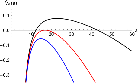
Figure 1: The effective potential $\tilde{V}_{K}(a)$ for a bouncing universe (black), emergent universe (red), singular universe (blue), for $K=0$, $w=1/3$, $g_{\ast}=0.1$, $\lambda_{\ast}=-0.5$ and $m=3$. Black, red and blue correspond to $\Lambda_{0}=2\times 10^{-4}$, $\Lambda_{0}=8.3\times 10^{-4}$ and $\Lambda_{0}=1.5\times 10^{-3}$ respectively.

The most interesting case is the emergent universe scenario. The key feature of this model lies in a past-eternal inflationary phase which naturally follows an initial quasi-static state. The universe thus starts at some minimum scale factor, $a_{b}>0$. Subsequently it inflates and evolves according to the standard cosmology as predicted by General Relativity. This possibility arises when eq. (21) has a double zero at some $a_{b}>0$ such that $\tilde{V}_{K}^{\prime\prime}(a_{b})<0$, and the special condition $\dot{a}_{b}=\ddot{a}_{b}=0$ holds. This case is represented by the red line in Fig. 1.

In the case of an early universe filled with pure radiation, the solutions to eq. (21) can be written as follows

$$a_{b}^{2}=-\frac{G_{0}\Lambda_{0}+g_{\ast}(\lambda_{\ast}-3K)}{2g_{\ast}\Lambda_{0}}\pm\sqrt{\left(\frac{G_{0}\Lambda_{0}-g_{\ast}(\lambda_{\ast}-3K)}{2g_{\ast}\Lambda_{0}}\right)^{2}-\frac{8\pi m\,G_{0}}{\Lambda_{0}}}\;\;.$$ (22)

Imposing the uniqueness of this solution basically fixes the integration constant $m$ introduced in eq. (4). Moreover, we require $a_{b}^{2}$ to be positive, as well as $\tilde{V}^{\prime\prime}_{K}(a_{b})<0$. The condition to realize a non-trivial ($\tilde{V}_{K}(a)\leq 0$) emergent universe thus reads

$$\lambda_{\ast}-3K<-\frac{G_{0}\Lambda_{0}}{g_{\ast}}\;\;.$$ (23)

In the classical case $\lambda_{\ast}=0$ and hence, assuming that the infrared values of the cosmological constant $\Lambda_{0}$ and Newton’s coupling $G_{0}$ are positive, an emergent universe is possible only for positive values of the spatial curvature, $K>0$. On the contrary, the Asymptotic Safety scenario is based on the existence of a NGFP, so that $\lambda_{\ast}\neq 0$. In the latter case the emergent universe can be realized by all allowed topologies of the spatial slices, $K=-1,0,1$, provided that $\lambda_{\ast}<0$. Remarkably, although $\lambda_{\ast}>0$ for “pure gravity”, in the case of gravity-matter systems the value of $\lambda_{\ast}$ depends on the matter content of the theory. In particular, when gravity is minimally coupled to the matter fields of the Standard Model (or its minor modifications), the gravitational RG flow computed in the ADM-framework has a unique (UV-attractive) NGFP with $\lambda_{\ast}<0$ Biemans et al. (2017b). In addition, a cosmological constant which attains negative values in the ultraviolet limit is necessary to ensure the compatibility of Asymptotic Safety with the latest Planck data Bonanno et al. (tion).

Provided that the condition (23) holds, in the case of an emergent universe eq. (17) reads

$$\dot{a}^{2}=-\frac{g_{\ast}\Lambda_{0}\left(a^{2}-a_{b}^{2}\right)^{2}}{3\left({G_{0}}-g_{\ast}a^{2}\right)}$$ (24)

where the minimum scale factor $a_{b}$ is given by

$$a_{b}=\sqrt{-\frac{G_{0}\Lambda_{0}+g_{\ast}(\lambda_{\ast}-3K)}{2g_{\ast}\Lambda_{0}}}\;\;.$$ (25)

Note that the condition $\tilde{V}_{K}(a)\leq 0$ implies

$$a^{2}\geq a_{b}^{2}>\frac{G_{0}}{g_{\ast}}\;\;.$$ (26)

Here the quantity $({G_{0}}/{g_{\ast}})$ corresponds to the value of $a(t)$ at which the anomalous dimension (9) is $\eta=-1$. The value of the minimal length $a_{b}$ cannot exceed this limit.

In order to understand how the universe evolves in the proximity of $a_{b}$, i.e. at the very beginning of its evolution, one can linearize the quantum-corrected equation (17) around $a_{b}$. The resulting approximate equation reads

$$\dot{a}^{2}=\frac{4{g_{\ast}}a_{b}^{2}\Lambda_{0}}{3\left({g_{\ast}}a_{b}^{2}-{G_{0}}\right)}(a-a_{b})^{2}$$ (27)

and its general solution is

$$a(t)=a_{b}+\epsilon\,\mathrm{exp}\left\{\sqrt{\frac{4{g_{\ast}}a_{b}^{2}\Lambda_{0}}{3\left({g_{\ast}}a_{b}^{2}-{G_{0}}\right)}}\;t\right\}\;\;,$$ (28)

$\epsilon$ being an integration constant. As it is clear from eq. (28), the emergent universe scenario associated with eq. (21) gives rise to an exponential evolution of the scale factor and no ad hoc inflation is needed. In particular, the density parameter can be written as

$$\Omega-1=\frac{3\left({g_{\ast}}a_{b}^{2}-{G_{0}}\right)K}{4{g_{\ast}}a_{b}^{4}\Lambda_{0}}\;e^{-2N_{e}}$$ (29)

where the number of e-folds $N_{e}$ reads

$$N_{e}\simeq\mathrm{log}\left(\frac{\epsilon}{a_{b}}\,\mathrm{exp}\left\{\sqrt{\frac{4{g_{\ast}}a_{b}^{2}\Lambda_{0}}{3\left({g_{\ast}}a_{b}^{2}-{G_{0}}\right)}}\;t_{e}\right\}\right)\;\;,$$ (30)

$t_{e}$ being the cosmic time at the inflation exit.

V Conclusions

In this work we discussed a class of homogeneous cosmologies consistent with an ADM Renormalization Group evolution. Our quantum-corrected Friedmann equation provides a new family of bouncing cosmologies which are valid near the basin of attraction of the NGFP and avoid the classical singularity. Emergent universe solutions are also possible depending on the renormalized trajectories around the NGFP. These latter are determined by only two parameters, which are in principle fixed by observations. In particular we showed that our emergent universe models do not depend on the topologies of the spatial sections and do not rely on the presence of exotic matter.

The Dirac analysis shows that the constraint algebra of the quantum-deformed dynamical variables is closed. An interesting question is the generalization of our approach beyond the mini-superspace approximation used in this work. We hope to address this issue in a future work.

References

- Brandenberger (2011) R. H. Brandenberger, ArXiv e-prints (2011), arXiv:1103.2271 .
- Planck Collaboration et al. (2016) Planck Collaboration, P. A. R. Ade, N. Aghanim, M. Arnaud, M. Ashdown, J. Aumont, C. Baccigalupi, A. J. Banday, R. B. Barreiro, J. G. Bartlett, and et al., A&A 594, A13 (2016), arXiv:1502.01589 .
- Hawking and Penrose (1970) S. W. Hawking and R. Penrose, Proceedings of the Royal Society of London Series A 314, 529 (1970).
- Borde et al. (2003) A. Borde, A. H. Guth, and A. Vilenkin, Physical Review Letters 90, 151301 (2003), gr-qc/0110012 .
- Mukhanov and Brandenberger (1992) V. Mukhanov and R. Brandenberger, Physical Review Letters 68, 1969 (1992).
- Brandenberger et al. (1993) R. Brandenberger, V. Mukhanov, and A. Sornborger, Phys. Rev. D 48, 1629 (1993), gr-qc/9303001 .
- Novello and Bergliaffa (2008) M. Novello and S. E. P. Bergliaffa, Phys. Rep. 463, 127 (2008), arXiv:0802.1634 .
- Cai et al. (2009) Y.-F. Cai, T. Qiu, J.-Q. Xia, H. Li, and X. Zhang, Phys. Rev. D 79, 021303 (2009), arXiv:0808.0819 .
- Cai and Zhang (2009) Y.-F. Cai and X. Zhang, JCAP 6, 003 (2009), arXiv:0808.2551 .
- Cai et al. (2007) Y.-F. Cai, T. Qiu, X. Zhang, Y.-S. Piao, and M. Li, Journal of High Energy Physics 10, 071 (2007), arXiv:0704.1090 [gr-qc] .
- Lin et al. (2011) C. Lin, R. H. Brandenberger, and L. Perreault Levasseur, JCAP 4, 019 (2011), arXiv:1007.2654 [hep-th] .
- Biswas et al. (2006) T. Biswas, A. Mazumdar, and W. Siegel, JCAP 3, 009 (2006), hep-th/0508194 .
- Easson et al. (2011) D. A. Easson, I. Sawicki, and A. Vikman, JCAP 11, 021 (2011), arXiv:1109.1047 [hep-th] .
- Qiu et al. (2011) T. Qiu, J. Evslin, Y.-F. Cai, M. Li, and X. Zhang, JCAP 10, 036 (2011), arXiv:1108.0593 [hep-th] .
- Cai et al. (2012) Y.-F. Cai, D. A. Easson, and R. Brandenberger, JCAP 8, 020 (2012), arXiv:1206.2382 [hep-th] .
- Ayón-Beato et al. (2016) E. Ayón-Beato, F. Canfora, and J. Zanelli, Physics Letters B 752, 201 (2016), arXiv:1509.02659 [gr-qc] .
- Harrison (1967) E. R. Harrison, MNRAS 137, 69 (1967).
- Ellis and Maartens (2004) G. F. R. Ellis and R. Maartens, Class. Quant. Grav. 21, 223 (2004), arXiv:gr-qc/0211082 [gr-qc] .
- Ellis et al. (2004) G. F. R. Ellis, J. Murugan, and C. G. Tsagas, Class. Quant. Grav. 21, 233 (2004), arXiv:gr-qc/0307112 [gr-qc] .
- Barrow et al. (2003) J. D. Barrow, G. F. R. Ellis, R. Maartens, and C. G. Tsagas, Classical and Quantum Gravity 20, L155 (2003), gr-qc/0302094 .
- Eddington (1930) A. S. Eddington, MNRAS 90, 668 (1930).
- Reuter and Saueressig (2012) M. Reuter and F. Saueressig, New Journal of Physics 14, 055022 (2012), arXiv:1202.2274 [hep-th] .
- Reuter and Saueressig (2013) M. Reuter and F. Saueressig, in Lecture Notes in Physics, Berlin Springer Verlag, Lecture Notes in Physics, Berlin Springer Verlag, Vol. 863, edited by G. Calcagni, L. Papantonopoulos, G. Siopsis, and N. Tsamis (2013) p. 185, arXiv:1205.5431 [hep-th] .
- Niedermaier and Reuter (2006) M. Niedermaier and M. Reuter, Living Reviews in Relativity 9, 5 (2006).
- Percacci (2011) R. Percacci, ArXiv e-prints (2011), arXiv:1110.6389 [hep-th] .
- Litim (2011) D. F. Litim, Philosophical Transactions of the Royal Society of London Series A 369, 2759 (2011), arXiv:1102.4624 [hep-th] .
- Weinberg (1976) S. Weinberg, Erice Subnuclear Physics (1976).
- Weinberg (1979) S. Weinberg, in General Relativity: An Einstein centenary survey, edited by S. W. Hawking and W. Israel (1979) pp. 790–831.
- Souma (1999) W. Souma, Progress of Theoretical Physics 102, 181 (1999), hep-th/9907027 .
- Reuter and Saueressig (2002) M. Reuter and F. Saueressig, Phys. Rev. D 65, 065016 (2002), hep-th/0110054 .
- Lauscher and Reuter (2002) O. Lauscher and M. Reuter, Phys. Rev. D 66, 025026 (2002), hep-th/0205062 .
- Codello et al. (2008) A. Codello, R. Percacci, and C. Rahmede, International Journal of Modern Physics A 23, 143 (2008), arXiv:0705.1769 [hep-th] .
- Machado and Saueressig (2008) P. F. Machado and F. Saueressig, Phys. Rev. D 77, 124045 (2008), arXiv:0712.0445 .
- Falls et al. (2013) K. Falls, D. F. Litim, K. Nikolakopoulos, and C. Rahmede, ArXiv e-prints (2013), arXiv:1301.4191 [hep-th] .
- Eichhorn (2015) A. Eichhorn, Journal of High Energy Physics 4, 96 (2015), arXiv:1501.05848 [gr-qc] .
- Falls and Ohta (2016) K. Falls and N. Ohta, Phys. Rev. D 94, 084005 (2016), arXiv:1607.08460 [hep-th] .
- Dietz and Morris (2013) J. A. Dietz and T. R. Morris, Journal of High Energy Physics 1, 108 (2013), arXiv:1211.0955 [hep-th] .
- Ohta et al. (2015) N. Ohta, R. Percacci, and G. P. Vacca, Phys. Rev. D 92, 061501 (2015), arXiv:1507.00968 [hep-th] .
- Ohta et al. (2016) N. Ohta, R. Percacci, and G. P. Vacca, European Physical Journal C 76, 46 (2016), arXiv:1511.09393 [hep-th] .
- Codello and Percacci (2006) A. Codello and R. Percacci, Physical Review Letters 97, 221301 (2006), hep-th/0607128 .
- Benedetti et al. (2009) D. Benedetti, P. F. Machado, and F. Saueressig, Modern Physics Letters A 24, 2233 (2009), arXiv:0901.2984 [hep-th] .
- Saueressig et al. (2011) F. Saueressig, K. Groh, S. Rechenberger, and O. Zanusso, ArXiv e-prints (2011), arXiv:1111.1743 [hep-th] .
- Gies et al. (2016) H. Gies, B. Knorr, S. Lippoldt, and F. Saueressig, Physical Review Letters 116, 211302 (2016), arXiv:1601.01800 [hep-th] .
- Rechenberger and Saueressig (2012) S. Rechenberger and F. Saueressig, Phys. Rev. D 86, 024018 (2012), arXiv:1206.0657 [hep-th] .
- Christiansen et al. (2014) N. Christiansen, D. F. Litim, J. M. Pawlowski, and A. Rodigast, Physics Letters B 728, 114 (2014).
- Manrique et al. (2011) E. Manrique, S. Rechenberger, and F. Saueressig, Physical Review Letters 106, 251302 (2011), arXiv:1102.5012 [hep-th] .
- Biemans et al. (2017a) J. Biemans, A. Platania, and F. Saueressig, Phys. Rev. D 95, 086013 (2017a), arXiv:1609.04813 [hep-th] .
- Biemans et al. (2017b) J. Biemans, A. Platania, and F. Saueressig, Journal of High Energy Physics 5, 93 (2017b), arXiv:1702.06539 [hep-th] .
- Houthoff et al. (2017) W. B. Houthoff, A. Kurov, and F. Saueressig, European Physical Journal C 77, 491 (2017), arXiv:1705.01848 [hep-th] .
- Reuter (1998) M. Reuter, Phys. Rev. D 57, 971 (1998), hep-th/9605030 .
- Reuter and Wetterich (1994) M. Reuter and C. Wetterich, Nuclear Physics B 417, 181 (1994).
- Berges et al. (2002) J. Berges, N. Tetradis, and C. Wetterich, Phys. Rep. 363, 223 (2002), hep-ph/0005122 .
- Benedetti et al. (2011) D. Benedetti, K. Groh, P. F. Machado, and F. Saueressig, Journal of High Energy Physics 6, 79 (2011), arXiv:1012.3081 [hep-th] .
- Bonanno and Reuter (2002a) A. Bonanno and M. Reuter, Physics Letters B 527, 9 (2002a), astro-ph/0106468 .
- Bonanno and Reuter (2002b) A. Bonanno and M. Reuter, Phys. Rev. D 65, 043508 (2002b), hep-th/0106133 .
- Dou and Percacci (1998) D. Dou and R. Percacci, Classical and Quantum Gravity 15, 3449 (1998), hep-th/9707239 .
- Guberina et al. (2003) B. Guberina, R. Horvat, and H. Štefančić, Phys. Rev. D 67, 083001 (2003), hep-ph/0211184 .
- Reuter and Weyer (2004a) M. Reuter and H. Weyer, Phys. Rev. D 70, 124028 (2004a), hep-th/0410117 .
- Reuter and Weyer (2004b) M. Reuter and H. Weyer, Phys. Rev. D 69, 104022 (2004b), hep-th/0311196 .
- Babić et al. (2005) A. Babić, B. Guberina, R. Horvat, and H. Štefančić, Phys. Rev. D 71, 124041 (2005), astro-ph/0407572 .
- Reuter and Saueressig (2005) M. Reuter and F. Saueressig, JCAP 9, 012 (2005), hep-th/0507167 .
- Bonanno et al. (2006) A. Bonanno, G. Esposito, C. Rubano, and P. Scudellaro, Classical and Quantum Gravity 23, 3103 (2006), astro-ph/0507670 .
- Bonanno and Reuter (2007) A. Bonanno and M. Reuter, JCAP 8, 024 (2007), arXiv:0706.0174 [hep-th] .
- Weinberg (2010) S. Weinberg, Phys. Rev. D 81, 083535 (2010), arXiv:0911.3165 [hep-th] .
- Cai and Easson (2011) Y. F. Cai and D. A. Easson, Phys. Rev. D 84, 103502 (2011), arXiv:1107.5815 [hep-th] .
- Bonanno et al. (2011) A. Bonanno, A. Contillo, and R. Percacci, Classical and Quantum Gravity 28, 145026 (2011), arXiv:1006.0192 [gr-qc] .
- Bonanno (2012) A. Bonanno, Phys. Rev. D 85, 081503 (2012), arXiv:1203.1962 [hep-th] .
- Bonanno and Platania (2015) A. Bonanno and A. Platania, Physics Letters B 750, 638 (2015), arXiv:1507.03375 [gr-qc] .
- Cai et al. (2013) Y. F. Cai, Y. C. Chang, P. Chen, D. A. Easson, and T. Qiu, Phys. Rev. D 88, 083508 (2013), arXiv:1304.6938 [hep-th] .
- Bonanno and Saueressig (2017) A. Bonanno and F. Saueressig, Comptes Rendus Physique 18, 254 (2017), arXiv:1702.04137 [hep-th] .
- Kofinas and Zarikas (2016) G. Kofinas and V. Zarikas, Phys. Rev. D 94, 103514 (2016), arXiv:1605.02241 [gr-qc] .
- Arnowitt et al. (1959) R. Arnowitt, S. Deser, and C. W. Misner, Physical Review 116, 1322 (1959).
- Arnowitt et al. (2008) R. Arnowitt, S. Deser, and C. W. Misner, General Relativity and Gravitation 40, 1997 (2008), gr-qc/0405109 .
- Dimakis et al. (2014) N. Dimakis, T. Christodoulakis, and P. A. Terzis, Journal of Geometry and Physics 77, 97 (2014), arXiv:1311.4358 [gr-qc] .
- York (1986) J. W. York, Foundations of Physics 16, 249 (1986).
- DeWitt (1967) B. S. DeWitt, Physical Review 160, 1113 (1967).
- Dirac (1966) P. A. M. Dirac, Lectures on quantum field theory (Yeshiva Univ., 1966).
- Anderson and Bergmann (1951) J. L. Anderson and P. G. Bergmann, Physical Review 83, 1018 (1951).
- Bergmann (1949) P. G. Bergmann, Physical Review 75, 680 (1949).
- Bonanno and Reuter (2000) A. Bonanno and M. Reuter, Phys. Rev. D 62, 043008 (2000), hep-th/0002196 .
- Bonanno et al. (tion) A. Bonanno, A. Platania, and F. Saueressig, (in preparation).