DASHMM Accelerated Adaptive Fast Multipole Poisson-Boltzmann Solver on Distributed Memory Architecture

Abstract

We present an updated version of the AFMPB package for fast calculation of molecular solvation-free energy. The main feature of the new version is the successful adoption of the DASHMM library, which enables AFMPB to operate on distributed memory computers. As a result, the new version can easily handle larger molecules or situations with higher accuracy requirements. To demonstrate the updated code, we applied the new version to a dengue virus system with more than one million atoms and a mesh with approximately 20 million triangles, and were able to reduce the time-to-solution from 10 hours reported in the previous release on a shared memory computer to less than 30 seconds on a Cray XC30 cluster using $12,288$ cores.

PROGRAM SUMMARY/NEW VERSION PROGRAM SUMMARY

Program Title: Distributed AFMPB
Licensing provisions: GNU General Public License, version 3
Programming language: C++
Supplementary material:
Journal reference of previous version: AEGB_v2_0
Does the new version supersede the previous version?: Yes
Reasons for the new version: Memory requirement and time-to-solution for large molecules of interest exceed the capacity of shared memory computers.
Summary of revisions: The revision extends the AFMPB to operate on distributed memory computers using the DASHMM [1, 2] library.
Nature of problem: Numerical solution of the linearized Poisson-Boltzmann equation that describes electrostatic interactions of molecular systems in ionic solutions.
Solution method: The linearized Poisson-Boltzmann equation is reformulated as a boundary integral equation and is subsequently discretized using the node-patch scheme. The resulting linear system is solved using GMRES. Within each iteration, the matrix-vector multiplication is accelerated using the DASHMM library on distributed memory computers.

1 Introduction

The Poisson-Boltzmann (PB) continuum electrostatic model has been adopted in many simulation tools for theoretical studies of electrostatic interactions between biomolecules such as proteins and DNAs in aqueous solutions. Various numerical techniques have been developed to solve the PB equations and help elucidate the electrostatic role in many biological processes, such as enzymatic catalysis, molecular recognition and bioregulation. Packages such as DelPhi [1, 2], MEAD [3], UHBD [4, 5], PBEQ [6], ZAP [7], and MIBPB [8] are based on finite-difference methods. Packages such as the Adaptive Poisson-Boltzmann Solver (APBS) [9] is based on finite volume/multigrid methods. In a circumstance where the linearized PB is applicable, the partial differential equations can be reformulated into a set of surface integral equations (IEs) by using Green’s theorem and potential theory. The unknowns in the IEs are located on the molecular surface, and the resulting discretized linear system can be solved very efficiently and accurately with certain fast convolution algorithms, such as the fast multipole method (FMM). This strategy has been implemented in the Adaptive Fast Multipole Poisson-Boltzmann (AFMPB) solver.

The AFMPB solver was first released as a sequential package written in Fortran [10]. A major update was released in 2015 [11] that used the Cilk runtime for parallelization on shared memory computers and provided built-in surface mesh generation capability. Over time, the target applications of AFMPB grew larger and required higher accuracy, which meant that it became difficult or impossible to find a shared memory computer with sufficient memory or processing capacity to solve the problems of interest. This paper presents a major update to AFMPB v. 2.0 [11] that extends its operation to distributed memory architectures.

To easily create a distributed version of AFMPB, the Dynamic Adaptive System for Hierarchical Multipole Method (DASHMM) [12, 13] library was adopted as the central driver of the multipole methods used by AFMPB. DASHMM is built on top of the asynchronous many-tasking HPX-5 [14, 15] runtime system. It is fine-grained, data-driven, and has very good strong-scaling. More importantly, the DASHMM programmer interface is independent of HPX-5 and no knowledge of the runtime is required from its end-users. As a result, upgrading AFMPB to use DASHMM was simple and fast.

In addition to the distribution of the FMM computation, the use of GMRES by AFMPB needed to be upgraded to work in distributed memory architectures. Before this update, AFMPB used SPARSKIT’s [16] GMRES implementation. This sequential, Fortran, implementation was replaced with a straightforward, fully-distributed GMRES patterned after the original SPARSKIT implementation.

These changes allow the new version of AFMPB to handle larger molecules or situations with higher accuracy requirements that were unfeasible on shared memory computers.

The organization of this paper is as follows. Section 2 reviews the mathematical models and discretization methods adopted in AFMPB and where DASHMM can be applied. Section 3 describes how DASHMM is integrated into AFMPB. Section 4 provides installation guide and job examples. Section 5 shows numerical results on two molecules. Section 6 concludes the paper.

2 Overview of the AFMPB Solver

The electrostatic force is considered to play an important role in the interactions and dynamics of molecular systems in aqueous solution. In the Poisson equation model, when the charge density that describes the electrostatic effects on the solvent outside the molecules is approximated by a Boltzmann distribution, the continuum nonlinear Poisson-Boltzmann (PB) equation assumes the following form

$$-\nabla\cdot(\epsilon\nabla\phi)+\bar{\kappa}^{2}\sinh(\phi)=\sum_{k=1}^{M}q_{k}\delta(r-r_{k})$$ (1)

In the formula, the molecule is represented by $M$ point charges $\{q_{k}\}$ located at $\{r_{k}\}$, $\epsilon$ is the position-dependent dielectric constant, $\phi$ is the electrostatic potential at location $r$, $\bar{\kappa}$ is the modified Debye-Hückel parameter, where $\bar{\kappa}=0$ in the molecule region and $\bar{\kappa}=\sqrt{\epsilon}\kappa$ in the solution region, and $\kappa$ is the inverse of the Debye-Hückel screening length determined by the ionic strength of the solution. When the electrostatic potentials are small, the linearized Poisson-Boltzmann (LPB) equation

$$-\nabla\cdot(\epsilon\nabla\phi)+\bar{\kappa}^{2}\phi=\sum_{k=1}^{M}q_{k}\delta(r-r_{k})$$ (2)

becomes valid, equipped with the interface conditions $[\phi]=0$ (by the continuity of the potential) and $[\epsilon\frac{\partial\phi}{\partial n}]=0$ (by the conservation of flux). Here, $[\,\,]$ denotes the jump across the molecular surface and $\frac{\partial}{\partial n}$ is the outward (towards the solvent) normal direction at the surface.

Instead of solving (2) directly, the AFMPB package adopts an alternative reformulation that maps (2) into

$$\left(\frac{1}{2\bar{\epsilon}}+\frac{1}{2}\right)f_{p} =\oint_{S}\left[(G_{pt}-u_{pt})h_{t}-\left(\frac{1}{\bar{\epsilon}}\frac{\partial G_{pt}}{\partial n}-\frac{\partial u_{pt}}{\partial n}\right)f_{t}\right]dS_{t}$$

$$\qquad+\frac{1}{\epsilon_{ext}}\sum_{k=1}^{M}q_{k}G_{pk}$$

$$\left(\frac{1}{2\bar{\epsilon}}+\frac{1}{2}\right)h_{p} =\oint_{S}\left[\left(\frac{\partial G_{pt}}{\partial n_{0}}-\frac{1}{\bar{\epsilon}}\frac{\partial u_{pt}}{\partial n_{0}}\right)h_{t}-\frac{1}{\bar{\epsilon}}\left(\frac{\partial^{2}G_{pt}}{\partial n_{0}\partial n}-\frac{\partial^{2}u_{pt}}{\partial n_{0}\partial n}\right)f_{t}\right]dS_{t}+$$

$$\qquad\frac{1}{\epsilon_{ext}}\sum_{k=1}^{M}q_{k}\frac{\partial G_{pk}}{\partial n_{0}}$$ (3)

where

$$G_{pt}=\frac{1}{4\pi|r_{t}-r_{p}|},\quad u_{pt}=\frac{e^{-\kappa|r_{t}-r_{p}|}}{4\pi|r_{t}-r_{p}|},\quad f=\phi^{ext},\quad h=\frac{\partial\phi^{ext}}{\partial n},\quad\bar{\epsilon}=\frac{\epsilon_{ext}}{\epsilon_{int}},$$

and $n_{0}$ is the outward unit normal vector at point $p\in S$. This alternative reformulation is a Fredholm integral equation of the second kind, which provides the analytic foundation for a well-condition system of equations with an adequate discretization method.

Figure 1: Illustration of the node-patch scheme used to discretize boundary integral equation (3) in the AFMPB solver. For each node $v$, its patch is enclosed by the edges connecting the centroid of the elements which $v$ belongs to and the midpoints of the edges incident at $v$. When the nodes are far apart, such as $v_{1}$ and $v_{3}$, the integrands of the integrations (6) are taken as constant on the patch. When the nodes are close, such as $v_{1}$ and $v_{2}$, the integrations (6) are computed directly using detailed information of the patches.

The AFMPB solver adopts the node-patch scheme [17] to discretize the integral equation (3). The scheme first constructs a patch around each node and then assumes unknowns are constant on each patch. Specifically, the patch around node $v$, denoted by $\Delta S_{v}$, is constructed by connecting the centroid points of the elements that node $v$ belongs to and the midpoints of the edges that are incident to $v$. Figure 1 provides an illustration of the node-patch approach on mesh of triangular elements. In the figure, the node-patch for $v_{1}$ is formed from six surrounding triangular elements. Using the node-patch scheme, equation (3) can be discretized as

$$\left(\frac{1}{2\bar{\epsilon}}+\frac{1}{2}\right)f_{p} =\sum_{t}(A_{pt}h_{t}-B_{pt}f_{t})+\frac{1}{\epsilon_{ext}}\sum_{k}q_{k}G_{pk}$$

$$\left(\frac{1}{2\bar{\epsilon}}+\frac{1}{2}\right)h_{p} =\sum_{t}(C_{pt}h_{t}-D_{pt}f_{t})+\frac{1}{\epsilon_{ext}}\sum_{k}q_{k}G_{pk},$$ (4)

or in matrix-form,

$$\begin{bmatrix}(\frac{1}{2\bar{\epsilon}}+\frac{1}{2})I+B&-A\\ D&(\frac{1}{2\bar{\epsilon}}+\frac{1}{2})I-C\end{bmatrix}\begin{bmatrix}f\\ h\end{bmatrix}=\frac{1}{\epsilon_{ext}}\begin{bmatrix}\sum_{k}q_{k}G_{pk}\\ \sum_{k}q_{k}\frac{\partial G_{pk}}{\partial n_{0}}\end{bmatrix}$$ (5)

where

$$A_{pt} =\oint_{\Delta S_{t}}(G_{pt}-u_{pt})dS,$$

$$B_{pt} =\oint_{\Delta S_{t}}\left(\frac{1}{\bar{\epsilon}}\frac{\partial G_{pt}}{\partial n}-\frac{\partial u_{pt}}{\partial n}\right)dS$$

$$C_{pt} =\oint_{\Delta S_{t}}\left(\frac{\partial G_{pt}}{\partial n_{0}}-\frac{1}{\bar{\epsilon}}\frac{\partial u_{pt}}{\partial n_{0}}\right)dS$$

$$D_{pt} =\oint_{\Delta S_{t}}\frac{1}{\bar{\epsilon}}\left(\frac{\partial^{2}G_{pt}}{\partial n_{0}\partial n}-\frac{\partial^{2}u_{pt}}{\partial n_{0}\partial n}\right)dS.$$ (6)

and $I$ is the identity matrix. The discretized system is well-conditioned and can be solved efficiently using Krylov subspace methods. For (6), when $p$ and $t$ are far-away, such as $v_{1}$ and $v_{3}$ in Figure 1, the integrands in (6) are taken as constants; When $p$ and $t$ are close, such as $v_{1}$ and $v_{2}$ in Figure 1, each integration is computed directly and the computation requires detailed information on the constitution of the patch. For this reason, in the existing AFMPB solver, the near-field integrations are computed only once and saved.

The overall computation flow of the existing AFMPB solver can be summarized as follows:

1. Compute the right-hand side of (5) using the Fast Multipole Method (FMM) with single-layer and double-layer Laplace potentials.

2. For each pair of nodes $p$ and $t$ whose patch integrations (6) are near-field, compute and save $A_{pt}$, $B_{pt}$, $C_{pt}$, and $D_{pt}$.

3. Solve equation (5) using Krylov subspace method. For each matrix-vector multiplication,

   1. Compute the near-field contribution using the $\{A,B,C,D\}$ coefficients in the previous step.

   2. Compute the far-field contribution with four FMM calls, using single-/double-layer Laplace and Yukawa potentials.

3 DASHMM and AFMPB Integration

The main feature of the new version is the adoption of the Dynamic Adaptive System for Hierarchical Multipole Method (DASHMM) library that enables the AFMPB solver to operate on distributed memory computers. With the added resources, larger molecules or situations with higher accuracy requirements that were infeasible on shared memory computers before can be handled with ease, and the time-to-solution is significantly reduced. In this section, we first briefly review the features and capabilities of the existing DASHMM library (version 1.2.0) and then documents the extensions made to DASHMM during the integration process.

3.1 DASHMM 1.2.0

DASHMM is an open-source scientific software library that aims to provide an easy-to-use system that can provide scalable, efficient, and unified evaluations of general hierarchical multipole methods on both shared and distributed memory architectures. The latest public release of DASHMM is version 1.2.0 [13]. DASHMM leverages the asynchronous multi-tasking HPX-5 [14, 15] runtime system for asynchrony management. HPX-5 defines a broad API that covers most aspects of the system. Programs are organized as diffusive, message driven computation, consisting of a large number of lightweight threads and active messages, executed within the context of a global address space, and synchronized through the use of lightweight synchronization objects. The HPX-5 runtime is responsible for managing global allocation, address resolution, data and control dependence, scheduling lightweight threads and managing network traffic. Readers interested in more HPX-5 and DASHMM implementation details are referred to [12, 13]. For general end-science users, the DASHMM APIs are completely independent of HPX-5 and no knowledge of the runtime system is required. A basic use can be achieved simply through the Evaluator object

dashmm::Evaluator<SourceData, TargetData, Expansion, Method>

that takes source data, target data, expansion, and method as template parameters.

DASHMM comes with a set of widely used interaction types (kernels), including the Laplace, Yukawa, and the low-frequency Helmholtz kernels. It also provides three built-in methods: Barnes-Hut, the classical FMM, and an variant of FMM that uses exponential expansion [18], which is called FMM97 method in the library. The Laplace and Yukawa kernels and the FMM97 method are used by the AFMPB solver.

DASHMM also makes a distinction between the mathematical concept of an expansion, and the concept used in DASHMM. The mathematical concept is a truncated series of some form (e.g., spherical harmonics) that represents some potential and is referred as a View object. The concept of an expansion in DASHMM is wider: each expansion in DASHMM can contain multiple mathematical expansions. In other words, each expansion in DASHMM is a collection of Views, or referred as a ViewSet object. The views of a ViewSet can represent the same potential, each from a different perspective, which is the case for exponential expansions in the FMM97 method. The views of a ViewSet can also represent different potentials, which is quite useful in the AFMPB solver. This means that the four FMM kernel evaluations within each iteration step can be processed concurrently.

3.2 New Kernels and Methods

To complete its computation, AFMPB required the implementation of two kernels and one method for use with the DASHMM framework. These new kernels and methods are an example of the extensibility of DASHMM. As long as these new classes conform to the required interface needed by DASHMM, the library can provide a parallel distributed FMM evaluation. These new kernels and method are not included in DASHMM, but rather are application specific extensions usable by DASHMM.

New kernels: AFMPB solves (5) using a Krylov subspace method. Applying the left-hand side matrix to each input vector involves four different kernels. In addition to the single-layer Laplace and Yukawa kernels already built into the DASHMM library, AFMPB implemented operators for the double-layer Laplace and double-layer Yukawa kernels. Notice that the multipole/local expansion for the double-layer potentials share the same form as the single-layer potentials. This means, only three operators are needed for each new kernel: (1) S_to_M operator that generates a multipole expansion from a set of source points; (2) S_to_L operator that generates a local expansion from a set of source points; (3) L_to_T operator that evaluates the local expansion at target points. For the reason discussed next, the M_to_T operator is not needed.

New Method: In adaptive FMM, each target box $B_{t}$ is associated with four types of lists [19] of source boxes. Particularly, a box $B_{s}$ is said to be in list-3 of $B_{t}$ if $B_{t}$ is well separated from $B_{s}$ but is not well separated from the parent of $B_{s}$. This is very cost effective because the multipole expansion is used at the earliest possible time. In the AFMPB solver, however, list-3 boxes have to be processed the same way as list-1 boxes using the S_to_T operator to achieve the required accuracy. This only calls a slight modification of the built-in FMM97 method, but it has an impact on the strong-scaling performance (see Section 5).

3.3 DASHMM extensions

In addition to new kernels and methods to be used by DASHMM, AFMPB drove some improvements to the DASHMM library. These are outlined below.

New API: In DASHMM 1.2.0, the multipole evaluation is done in a monolithic way through the single evaluate method of the Evaluator class. It first constructs the auxiliary structures, such as the dual tree and the directed acyclic graph (DAG), and then evaluates the DAG. This approach provides an easy-to-use and complete evaluation of a given multipole method. However, this one-size-fits-all approach is not well tuned for iterative methods that uses the same DAG multiple times with different input data. To address this, DASHMM now supports evaluation split into phases, including:

create_tree

Partition the source and target points into two trees. The trees can be identical, partially overlapping, or completely disjoint. In AFMPB, the right-hand side of (5) is a case where the sources (atoms inside the molecule) are completely disjoint from the targets (mesh nodes on the molecule surface), and the left-hand side of (5) is a case where the sources and targets are the same (mesh nodes on the molecular surface).

create_DAG

This method takes the handle of the tree constructed from create_tree and a given multipole method object to connect the trees into a DAG.

execute_DAG

This method performs the evaluation of the multipole method.

reset_DAG

This method resets various DASHMM internal control objects. Once complete, the DAG is ready to execute a new round of execution.

destroy_DAG

This method destroys the DAG.

destroy_tree

This method destroys the dual trees.

By separating the evaluation into phases AFMPB can build the tree and DAG only once, and evaluate that DAG repeatedly. This saves the overhead of building an identical tree and DAG for each iteration.

New Functionality: The previous AFMPB solver first generates the $\{A,B,C,D\}$ coefficients for the near-field integration before starting the iterative solution phase. This synchronization barrier blocks the far-field evaluation of the first matrix-vector multiplication of the iterative solve, and increases the overall execution time. The updated version of AFMPB removes this barrier. AFMPB directly enters the iterative solve phase, generates and saves the $\{A,B,C,D\}$ coefficients for future iterations while making progress on the far-field evaluation. This suggested additional functionality from DASHMM: the detailed patch information associated with each node is needed only in the first iteration and one should avoid communicating unnecessary large messages. DASHMM addresses this by introducing the Serializer object, which has three member functions:

size

This takes a handle to the object in question and returns the size in bytes of the serialized object.

serialize

This serializes the given object into the buffer provided and then returns the address after the serialized data.

deserialize

This deserializes the given object into the buffer provided and then returns the address after the data used in the deserialization.

DASHMM now defines a method, set_manager, on its Array type that allows the array to update its binding to a Serializer during the course of execution. Two Serializer objects are defined in the new version of AFMPB: one serializes detailed patch information and is used only in the first iteration, and the other serializes the new input vector generated from the Krylov solver in the successive iterations.

3.4 GMRES

AFMPB uses the Generalized minimal residual (GMRES) from SPARSKIT [16] to solve the discretized system (5). SPARSKIT is written in Fortran and does not operate on distributed memory computers. When the bulk of computation in AFMPB becomes distributed, the GMRES operation must also become distributed. For this reason, the new version of AFMPB also includes an implementation of restarted GMRES on distributed memory computers. The implementation follows closely to the one in SPARSKIT, skipping statements on preconditioners because (5) is a well-conditioned system resulting from the second kind Fredholm integral equation formulation.

We also note that in previous AFMPB versions, there are separate buffers to store the Krylov basis and the input to the multipole method. As the input to the multipole method is simply the last orthonormal basis formed, this extra storage is eliminated. Additionally, to reduce unnecessary communications, the Krylov basis are distributed exactly the same way as the mesh nodes. In other words, each Node object has a gmres member that stores the corresponding Krylov basis components.

4 Software Installation and Job Examples

4.1 Installation

The new version AFMPB depends on two external libraries: DASHMM and HPX-5. Version 4.1.0 of HPX-5 can be downloaded from https://hpx.crest.iu.edu/download. DASHMM is automatically downloaded by AFMPB when the application is built.

Users must install HPX-5 on their systems before installing the AFMPB solver. HPX-5 currently specifies two network interfaces: the ISend/IRecv interface with the MPI transport, and Put-with-completion (PWC) interface with the Photon transport. HPX-5 can be built with or without network transports. Assume that you have unpacked the HPX-5 source into the folder /path/to/hpx and wish to install the library into /path/to/install. Without network support, the following steps should build HPX-5 and install it.

1. cd /path/to/hpx

2. ./configure --prefix=/path/to/install

3. make

4. make install

To configure HPX-5 with MPI network, simply add --enable-mpi to the configure line. The configuration will search for the appropriate way to include and link to MPI.

1. HPX-5 will try and see if mpi.h and libmpi.so are available with no additional flags.

2. HPX-5 will test for an mpi.h and -lmpi in the current C_INCLUDE_PATH and {LD}_LIBRARY_PATH respectively.

3. HPX-5 will look for an ompi pkg-config package.

To configure HPX-5 with the Photon network, one adds --enable-photon to the configure line. HPX-5 does not provide its own distributed job launcher, so it is necessary to also use either the --enable-mpi or --enable-pmi option in order to build support for mpirun or aprun bootstrapping. Note that if you are building with the Photon network, the libraries for the given network interconnect you are targeting need to be present on the build system. The two supported interconnects are InfiniBand (libverbs and librdmacm) and Cray’s GEMINI and ARIES via uGNI (libugni). On Cray machines you also need to include the PHOTON_CARGS=‘‘--enable-ugni’’ to the configure line so that Photon builds with uGNI support. Finally, the --enable-hugetlbfs option causes the HPX-5 heap to be mapped with huge pages, which is necessary for larger heaps on some Cray Gemini machines.

Once the HPX-5 system is installed, assume the AFMPB source has been unpacked into the folder /path/to/afmpb, the package can be easily built using cmake (version 3.4 and above) as follows

1. mkdir build; cd build

2. cmake /path/to/afmpb

3. make

The previous commands will automatically download and build the DASHMM library, so no extra steps are required to satisfy that dependency.

4.2 Job Examples

Assume the exectuable is afmpb in this section. The solver can be used simply as

./afmpb --pqr-file=FILE

which will discretize the molecule using the built-in mesh generation tool and compute the potentials and solvent energy.

The other available options to the program are

–mesh-format=num

Available choices are 0, 1, 2. 0 indicates built-in mesh, 1 indicates MSMS mesh [20], and 2 indicates TMSmesh [21].

–mesh-file=FILE

Required if the mesh format is not zero.

–mesh-density=num

Specifies mesh density if built-in mesh is selected.

–probe-radius=num

Specifies probe radius if built-in mesh is selected.

–dielectric-interior=num

Specifies the interior dielectric constant.

–dielectric-exterior=num

Specifies the exterior dielectric constant.

–ion-concentration=num

Specifies the ionic concentration.

–temperature=num

Specifies the temperature

–surface-tension=num

Specifies the surface tension coefficient

–pressure=num

Specifies the pressure.

–accuracy=num

Specifies the accuracy of DASHMM, available choices are 3 and 6.

–rel-tolerance=num

Specifies relative tolerance of (7) for GMRES solver

–abs-tolerance=num

Specifies absolute tolerance of (7) for GMRES solver

–restart=num

Specifies the maximum dimension of Krylov space before it restarts.

–max-restart=num

Specifies the maximum number of times GMRES can restart.

–log-file=FILE

Name of the log file.

–potential-file=FILE

Name of the file containing computed potentials on each mesh node.

and they are also available by issuing ./afmpb --help from the command line.

Next, we use the 3K1Q molecule to be discussed in the next subsection to present some sample job scripts. On a cluster using Slurm workload manager, a job using 512 compute nodes looks like

#! /bin/bash -l
#SBATCH -p queue
#SBATCH -N 512
#SBATCH -J jobname
#SBATCH -o output
#SBATCH -e error
#SBATCH -t 00:10:00

srun -n 512 -c 48 ./afmpb --pqr-file=3k1q.pqr \
--mesh-format=2 --mesh-file=3k1q.off --log-file=3k1q.out512 \
--accuracy=6 --restart=79 --max-restart=5 --hpx-threads=24

It is worth noting that each compute node of the above cluster is equipped with two Intel Xeon E5 12-core CPUs with hyperthreading enabled. This means, Slurm sees 48 cores per compute node and the option -c 48 is to create one MPI process per compute node. As there are only 24 physical cores on each compute node, the option --hpx-threads=24 means HPX-5 will create only 24 scheduler threads, one for each physical core. If the above cluster were using the PBS workload manager, the script will look like

#! /bin/bash -l
#PBS -l nodes=512:ppn=48
#PBS -l walltime=00:10:00
#PBS -q queue

aprun -n 512 -d 48 ./afmpb ....

5 Numerical Examples

In this section, we demonstrate the accuracy and efficiency of the new AFMPB solver. AFMPB’s accuracy is demonstrated by considering a spherical case with known a analytic solution. AFMPB’s efficiency is demonstrated by applying the solver to two molecule systems: an aquareovirus virion 3K1Q and a dengue virus 1K4R. The results were collected from a Cray XC30 cluster at Indiana University. Each compute node has two Intel Xeon E5 12-core CPUs and 64 GB of DDR3 RAM. The HPX-5 runtime was configured with the Photon network.

The error tolerance for the GMRES solver is chosen to be

$$\epsilon_{rel}\|b\|_{2}+\epsilon_{abs},$$ (7)

where $b$ represents the right-hand side of (5), and the relative and absolute tolerance $\epsilon_{rel}$ and $\epsilon_{abs}$ depend on DASHMM’s accuracy, and the molecule system. When DASHMM computes with 6-digit accuracy, the lower bound for $\epsilon_{rel}$ is $10^{-6}$. When DASHMM computes with 3-digit accuracy, the lower bound for $\epsilon_{rel}$ is $10^{-3}$.

The sphere example used a sphere shaped molecule of 50Å  radius and a single atom carrying 50 elementary charge. The ionic concentraion is set to 0 mM. Under this assumption, the analytical solution of the polar energy is $-4046\,kcal/mol$. For the numerical solution, the surface is discretized into $1,310,720$ triangle elements and $655,362$ nodes. The results computed from the AFMPB solver are $-4065.42\,kcal/mol$ when DASHMM operates with 3-digit accuracy and $-4057.83\,kcal/mol$ when DASHMM oeprates with 6-digit accuracy. The relative differences are 0.47% and 0.29%, respectively.

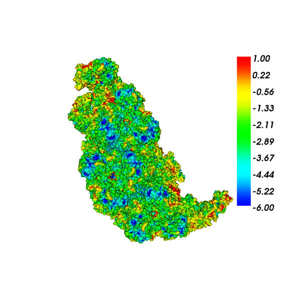
(a) 3K1Q

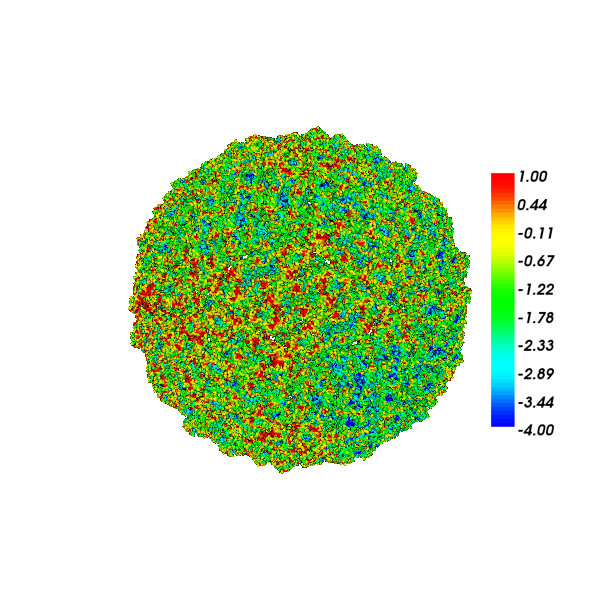
(b) 1K4R

Figure 2: Visualization of the surface potential of the aquareovirus virion (left) and dengue virus (right) systems using VCMM [22]. The surface mesh is generated using TMSmesh and the color bar for the surface potentials is in the unit of $kcal/mol.e$.

The surface mesh used for the 3K1Q and 1K4R examples were generated using TMSMesh [21]. The smaller molecule, 3K1Q, consists of $203,111$ atoms and its mesh consists of $7,788,246$ triangle elements and $3,888,281$ nodes. We were able to test the AFMPB solver on this molecule with both three and six digit accuracy requirements on DASHMM. At 3-digits of accuracy, the polar energy is $-8.81762\times 10^{4}\,kcal/mol$. At 6-digits of accuracy, the polar energy is $-8.81808\times 10^{4}\,kcal/mol$. The relative difference between the two accuracy requirement is 0.005%, indicating that the lower accuracy input on DASHMM is also acceptable for energy calculations. The larger molecule, 1K4R, consists of $1,082,160$ atoms and its mesh consists of $19,502,784$ triangle elements and $9,758,426$ nodes. For this molecule, we required three digits of accuracy and the polar energy is $-3.999067\times 10^{5}\,kcal/mol$. The output from the AFMPB package can be visualized by the package VCMM [22]. Figure 2 shows the visualization of the surface potentials of the two molecule systems. The potential results for the 3K1Q molecule on the left were computed with 6-digit accuracy on DASHMM.

To evaluate the strong scaling performance of the new AFMPB solver, we measure the execution time of the DASHMM evaluation phase and the GMRES phase. The DASHMM phase accumulates the total time spent on matrix-vector multiplication and the GMRES phase accumulates the time spent on inner production computation. Because the GMRES implementation is based on the modified Gram-Schmidt procedure with reorthogonalization, each inner product is a global barrier. Therefore, we also count the number of inner products performed in each solve. For each accuracy requirement, we started with the smallest number of compute nodes that could complete the computation, and used up to 512 compute nodes. GMRES was set to restart after 80 iterations and was allowed to restart five times. In all test cases, the solver converged well before that limit. For 3K1Q, GMRES took 11 iterations and 77 inner products to converge when DASHMM gave 3-digit accuracy, and 133 iterations and $4,803$ inner products to converge when DASHMM gave 6-digit accuracy. For 1K4R, GMRES took 10 iterations and 66 inner product to converge.

Figure 3: Execution times for DASHMM (matrix-vector multiplication) and GMRES (inner-product) for the three test cases on a Cray XC30 cluster. Each compute node (locality) consists of 24 cores and 64 GB of RAM. Molecule 3K1Q was tested with two different accuracy requirements for DASHMM. At 3-digit accuracy, GMRES took 11 iterations and 77 inner products to converge. At 6-digit accuracy, GMRES was restarted after 80 iterations and took 133 iterations and 4803 inner products to converge. Molecule 1K4R was tested with three digit accuracy requirement for DASHMM. The GMRES took 10 iterations and 66 inner products to converge.

Figure 3 shows the strong-scaling behavior for both the DASHMM and GMRES phases. Notice that the results for the GMRES phase depend on how DASHMM distributes the data. For instance, DASHMM didn’t do an optimal job distributing the data at 64 ranks for 3K1Q because the molecular surface is highly irregular (Figure 2). However, DASHMM distributed the data very well at 128 ranks as the strong scaling efficiency for GMRES is almost 100%. Nonetheless, each inner product is a global reduction and as the number of localities increases the computation will become insufficient to hide the network latency. This explains why all the GMRES curves flatten out at 512 localities.

Localities	3K1Q, 3-digit	3K1Q, 6-digit	1K4R, 3-digit
8	98%	N/A	N/A
16	97%	N/A	N/A
32	89%	N/A	N/A
64	57%	65%	95%
128	66%	98%	87%
256	45%	69%	60%
512	27%	42%	45%

Table 1: Strong scaling efficiency of the DASHMM part for 3K1Q and 1K4R test cases.

Table 1 summarizes the strong-scaling efficiency for the DASHMM phase of the AFMPB solver. Note that in all test cases, GMRES takes approximately 5% of the total execution and therefore the overall scaling is determined by that of DASHMM. For 3K1Q at lower accuracy requirement, the scaling efficiency is very good up to 32 localities and then decays rapidly. In fact, an input size around $4$ million points is very small and a single DASHMM evaluation could even fit in a single locality. Running it over distributed memory primarily adds memory capacity for the GMRES solver to work. For higher accuracy requirement or large molecule, the scaling efficiency can stay above 60% up to 256 localities, which is consistent with the ones reported in [13]. However, the efficiency at 512 localities are much worse.

The inferior scaling performance at 512 localities is caused by the fact that AFMPB does not distinguish types 1 and 3 lists in the adaptive FMM (see Section 3.3). In the adaptive FMM, if a source box $B_{s}$ is in list-3 for target box $B_{t}$, their interaction is handled by the M_to_T operator. If $B_{s}$ and $B_{t}$ are on different localities, one needs to communicate the multipole expansion of $B_{s}$ and the M_to_T operator has enough floating point operations (such as spherical harmonic evaluations) to offset the communication cost. In AFMPB, this interaction is handled by the S_to_T operator and $B_{s}$ needs to send “particles” (component of the Krylov basis) to $B_{t}$. First, $B_{s}$ can be a nonleaf box which contains many particles, making the message much larger. Second, once the $\{A,B,C,D\}$ coefficients are computed, for each particle information received, $B_{t}$ simply does four multiplications, which is not sufficient to offset the communication cost. The DASHMM team is currently working on extending the library to heterogeneous architectures. When complete, offloading the near-field interaction should be able to improve the scaling performance.

Finally, we point out that one often chooses restarted GMRES due to the memory limitation on storing the Krylov basis and it often takes more iterations to converge when GMRES restarts. When there are more resources available, one can afford not to restart GMRES and this could lead to shorter time-to-completion. For the 3K1Q example at 6-digit accuracy, we set GMRES to restart at 140 iterations and GMRES actually converged at iteration 89 and the execution time is 30% faster. The polar energy is $-8.83353\times 10^{4}\,kcal/mol$. Compared with the one obtained when GMRES restarted, the relative difference is less than 0.17%.

6 Conclusion

We have presented the DASHMM accelerated AFMPB solver for computing electrostatic properties and solvation energies of biomolecular systems. DASHMM leverages the global address space of the HPX-5 runtime system to provide a unified evaluation of the multipole methods on both shared and distributed memory computers. This enables the new version of AFMPB to operate on distributed memory computers while at the same time maintaining backward compatibility on shared memory computers. With the added processing units and memory capacity from distributed memory computers, larger molecules or situations requiring higher accuracy can be handled. We have tested the new solver on the dengue virus system reported in the previous release and was able to reduce the solving time from 10 hours down to about 30 seconds using $12,288$ cores.

The adoption of DASHMM as the FMM solver for AFMPB also revealed several issues requiring further study. A better treatment of the near-field interaction is needed to recover the scaling demonstrated by DASHMM in other contexts. One possible approach would be the use of accelerators for near field interactions. The current implementation of the GMRES solver follows closely the one in SPARSKIT. The modified Gram-Schmidt procedure involves many global synchronizations. Given the current breakdown of execution time devoted to FMM and GMRES, it should be possible to hide this synchronization overhead withing the matrix-vector multiplication using strategies mentioned in [23] and references therein.

References

- [1] J. DeBuhr, B. Zhang, A. Tsueda, V. Tilstra-Smith, and T. Sterling. DASHMM: Dynamic Adaptive System for Hierarchical Multipole Methods. Commun. Comput. Phys. 20 (2016) 1106-1126.
- [2] J. DeBuhr, B. Zhang, T. Sterling. Revision of DASHMM: Dynamic Adaptive System for Hierarchical Multipole Methods. Commun. Comput. Phys. Accepted.

References

- [1] C. Li, L. Li, J. Zhang, E. Alexov, Highly efficient and exact method for parallelization of grid-based algorithms and its implementation in DelPhi, J. Comput. Chem. 33 (2012) 1960–1966.
- [2] C. Li, M. Petukh, L. Li, E. Alexov, Continuous development of schemes for parallel computing of the electrostatics in biological systems: implementation in DelPhi, J. Comput. Chem. 34 (2013) 1949–1960.
- [3] D. Bashford, An object-oriented programming suite for electrostatic effects in biological molecules, Lecture Notes in Computer Science 1343 (1997) 233–240.
- [4] UHBD, http://mccammon.ucsd.edu/uhbd.html.
- [5] J. D. Madura, J. M. Briggs, R. C. Wade, M. E. Davis, B. A. Luty, A. Ilin, J. Antosiewicz, M. K. Gilson, B. Bagheri, L. R. Scott, J. A. McCammon, Electrostatics and diffusion of molecules in solution-simulation with the University of Houston Brownian Dynamics Program, Comput. Phys. Commun. 91 (1995) 57–95.
- [6] S. Jo, M. Vargyas, J. Vasko-Szedlar, B. Roux, V. Im, PBEQ-solver for online visualization of electrostatic potential of biomolecules, Nucleic Acids Research 36 (2008) 270–275.
- [7] J. A. Grant, B. T. Pickup, A. Nicholls, A smooth permittivity function for Poisson-Boltzmann solvation methods, J. Comput. Chem. 22 (2001) 608–640.
- [8] D. Chen, Z. Chen, C. Chen, W. Geng, G. Wei, MIBPB: A software package for electrostatic analysis, J. Comput. Chem. 32 (2011) 756–770.
- [9] APBS, http://www.poissonboltzmann.org/apbs.
- [10] B. Lu, X. Cheng, J. Huang, J. A. McCammon, AFMPB: Adaptive Fast Multipole Poisson-Boltzmann Solver, Comput. Phys. Commun. 181 (2010) 1150–1160.
- [11] B. Zhang, B. Peng, J. Huang, N. P. Pitsianis, X. Sun, B. Lu, Parallel AFMPB solver with automatic surface meshing for calculation of molecular solvation free energy, Comput. Phys. Commun. 190 (2015) 173–181.
- [12] J. DeBuhr, B. Zhang, A. Tsueda, V. Tilstra-Smith, T. Sterling, DASHMM: Dynamic Adaptive System for Hierarchical Multipole Methods, Communications in Computational Physics 20 (2016) 1106–1126.
- [13] J. DeBuhr, B. Zhang, T. Sterling, Revision of DASHMM: Dynamic Adaptive System for Hierarchical Multipole Mthods, Comm. Comput. Phys.
- [14] A. Kulkarni, L. Dalessandro, E. Kissel, A. Lumsdaine, T. Sterling, M. Swany, Network-managed virtual global address space for message-driven runtimes, in: Proceedings of the 25th International Symposium on High Performance Parallel and Distributed Computing (HPDC 2016), 2016.
- [15] E. Kissel, M. Swany, Photon: Remote memory access middleware for high-performance runtime systems, in: In Proceedings of the 1st Emerging Parallel and Distributed Runtime Systems and Middleware (IPDRM) Workshop, 2016.
- [16] http://www-users.cs.umn.edu/~saad/software/.
- [17] B. Lu, J. A. McCammon, Improved boundary element methods for Poisson-Boltzmann electrostatic potential and force calculations, J. Chem. Theory Comput. 3 (2007) 1134–1142.
- [18] L. Greengard, V. Rokhlin, A new version of the fast multipole method for the Laplace equation in three dimensions, Acta Numer. 6 (1997) 229–269.
- [19] J. Carrier, L. Greengard, V. Rokhlin, A fast adaptive multipole algorithm for particle simulations, SIAM J. Sci. Stat. Comp. 9 (1988) 669–686.
- [20] M. F. Scanner, A. J. Olson, J. C. Spehner, Reduced surface: an efficient way to compute molecular surfaces, Biopolymers 38 (1996) 305–320.
- [21] M. Chen, B. Lu, TMSmesh: A robust method for molecular surface mesh generation using a trace technique, J. Chem. Theory Comput. 7 (2011) 203–212.
- [22] S. Bai, B. Lu, VCMM: A visual tool for continuum molecular modeling, J. Mol. Graphics Modell. 50 (2014) 44–49.
- [23] P. Ghysels, T. J. Ashby, K. Meerbergen, W. Vanroose, Hiding global communication latency in the GMRES algorithm on massively parallel machines, SIAM. J. Sci. Comput. 35 (2013) C48–C71.