Ergodicity of the LLR method for the Density of States

Abstract

The LLR method is a novel algorithm that enables us to evaluate the density of states in lattice gauge theory. We present our study of the ergodicity properties of the LLR algorithm for the model of Yang Mills SU(3). We show that the use of the replica exchange method alleviates significantly the topological freeze-out that severely affects other algorithms.

1 Introduction

Monte Carlo (MC) importance sampling simulations are at the basis of lattice investigations and are one of the most powerful methods to study non-perturbative phenomena in quantum field theory. Despite their success, there is a number of known cases where they perform very poorly, for example in presence of an overlap problem, i.e. when the measure distribution induces on the update algorithm a poor sample of the portion of phase space relevant for the evaluation of the observables, or in case of quantities that cannot be expressed as expectation values over a probability measure like partition functions and free energies. Over the years many algorithms has been proposed that try to overcome some of these problems. In this work we investigate the ergodicity properties of a recently proposed method, the LLR method.

2 The method

Our method is based on the evaluation of the density of states, and has been recently proposed in Langfeld:2012ah ; Langfeld:2015fua . The density of states $\rho(\mathcal{S}\>\!)$ is defined via the functional integral

$$\rho(\mathcal{S}\>\!)=\int[D\phi]\,\delta(\mathcal{S}-S[\phi]),$$ (1)

where $\phi$ is some generic dynamical field variable, $[D\phi]$ is the path integral over the field configurations and $S[\phi]$ the action of the Euclidean quantum field theory. From the density of states it is possible to compute the partition function and expectation values of energy dependent observables via a simple one dimensional integration:

$$Z=\int\rm{d}\mathcal{S}\>\!\,e^{-\mathcal{S}\>\!}\rho(\mathcal{S}\>\!),$$ (2)

$$\langle\mathcal{O}\rangle=\frac{1}{Z}\int\rm{d}\mathcal{S}\>\!\,e^{-\mathcal{S}\>\!}\rho(\mathcal{S}\>\!)\,\mathcal{O}(\mathcal{S}\>\!),$$ (3)

while a bit more of care needs to be payed to evaluate generic observables (see sect.2.1).

The conceptual difference of this formulation with respect to classical Montecarlo techniques is that all the path integrals are evaluated on a micro-canonical ensemble, i.e. at fixed action.

2.1 The LLR method in a nutshell

The LLR algorithm gives access to a controllable approximation of the $\rho(\mathcal{S}\>\!)$ featuring strong convergence properties. The procedure can be summarised in the steps below.

For a given action range, partition the interval between $\mathcal{S}\>\!_{\mathrm{min}}$ and $\mathcal{S}\>\!_{\mathrm{max}}$ in $N$ subintervals and call $\mathcal{S}\>\!_{i}$ the center action value and $\delta_{S}=(\mathcal{S}\>\!_{\mathrm{max}}-\mathcal{S}\>\!_{\mathrm{min}})/N$, for evenly spread actions intervals. For each of the intervals evaluate

$$a_{i}=\left.\frac{d\,\ln\rho}{d\mathcal{S}\>\!}\right|_{\mathcal{S}\>\!=\mathcal{S}\>\!_{i}},$$ (4)

and from the knowledge of the coefficients $a_{i}$ reconstruct the log-linear approximation of the density of states as

$$\rho_{\mbox{\tiny LLR}}(\mathcal{S}\>\!)=\rho_{0}\prod_{i=1}^{k-1}e^{a_{i}\delta_{S}}{\rm{exp}}(a_{k}(\mathcal{S}\>\!-\mathcal{S}\>\!_{k})),\hskip 56.9055pt\mathcal{S}\>\!_{k}\leq\mathcal{S}\>\!<\mathcal{S}\>\!_{k+1}\,.$$ (5)

It can be shown that our approximation converges to the correct function: $\displaystyle\rho(\mathcal{S}\>\!)=\rho_{\mbox{\tiny LLR}}(\mathcal{S}\>\!)\,e^{c\,\delta_{S}^{2}}$ âalmost everywhereâ for $\delta_{S}\to 0$ (the $\rho(\mathcal{S}\>\!)$ is supposed to be almost everywhere $C_{2}$).

To evaluate the $a_{i}$ we first define:

$$\left\langle\kern-1.69998pt\left\langle\mathcal{S}\>\!-\mathcal{S}\>\!_{i}\right\rangle\kern-1.69998pt\right\rangle_{i}(a) = \frac{1}{{\cal N}}\int d\mathcal{S}\>\!\,e^{\frac{-(\mathcal{S}\>\!-\mathcal{S}\>\!_{i})^{2}}{2\delta_{S}^{2}}}\,\rho(\mathcal{S}\>\!)\,(\mathcal{S}\>\!-\mathcal{S}\>\!_{i})\,e^{a\mathcal{S}\>\!}$$ (6)

$$= \frac{1}{{\cal N}}\int[D\phi]\,e^{\frac{-(S[\phi]-\mathcal{S}\>\!_{i})^{2}}{2\delta_{S}^{2}}}\,(S[\phi]-\mathcal{S}\>\!_{i})\,e^{aS[\phi]}\;,$$ (7)

$${\cal N} = \int d\mathcal{S}\>\!\,e^{\frac{-(\mathcal{S}\>\!-\mathcal{S}\>\!_{i})^{2}}{2\delta_{S}^{2}}}\,\rho(\mathcal{S}\>\!)\,e^{a\mathcal{S}\>\!}=\int[D\phi]\,e^{\frac{-(S[\phi]-\mathcal{S}\>\!_{i})^{2}}{2\delta_{S}^{2}}}\,e^{aS[\phi]}\;,$$ (8)

where the double brackets $\left\langle\kern-1.69998pt\left\langle\dots\right\rangle\kern-1.69998pt\right\rangle$ represent the insertion of a strongly localised support function centred around the $\mathcal{S}\>\!_{i}$, in the present case a gaussian function. The $a_{i}$ are the zeros of the stochastic equation

$$\left\langle\kern-1.69998pt\left\langle\mathcal{S}\>\!-\mathcal{S}\>\!_{i}\right\rangle\kern-1.69998pt\right\rangle_{i}(a_{i})=0.$$ (9)

The stochastic nature of the latter is due to the determination of the double bracket expectation value, which can be accessed only through Monte Carlo estimates. The numerical solution of stochastic equations can be found using the iterative Robbins-Monro procedure robbins1951 . This begins with a guessed value $a^{(0)}_{i}$, which is updated using the iteration

$$a^{(n+1)}_{i}=a^{(n)}_{i}-c_{n}\left\langle\kern-1.69998pt\left\langle\mathcal{S}\>\!-\mathcal{S}\>\!_{i}\right\rangle\kern-1.69998pt\right\rangle_{i}(a^{(n)}_{i})\hskip 28.45274pt{\rm with}\;\sum_{n=0}^{\infty}c_{n}=\infty\;{\rm and}\;\sum_{n=0}^{\infty}c_{n}^{2}<\infty,$$ (10)

and converges in $L_{2}$, and hence in probability, to root of the equation:

$$\lim_{n\to\infty}a^{(n)}_{i}=a_{i},$$ (11)

for more details see robbins1951 .

Once the $a$âs are computed the density of states is reconstructed using eq.5 with error-bars determined using bootstrap resampling.

A few remarks are in order: the $\rho_{\mbox{\tiny LLR}}$ is an approximation of the correct density of state $O(\delta_{S}^{2})$ and it shows exponential error suppression: the relative approximation error does not depend on the magnitude, as a consequence this method works over several orders of magnitude. Once the $a_{i}$ have been evaluated, energy observables can be evaluated through direct integration of the density of states while generic observables can be evaluated through

$$\langle\mathcal{B}\rangle=\frac{1}{Z}\,\sum_{i}\delta_{S}\;\rho_{\mbox{\tiny LLR}}\left(\mathcal{S}\>\!_{i}\right)e^{-a_{i}\mathcal{S}\>\!_{i}}\;\left\langle\kern-1.69998pt\left\langle\mathcal{B}[\phi]\,e^{-(a_{i}+1)S[\phi]}\right\rangle\kern-1.69998pt\right\rangle+O(\delta_{S}^{2}),$$ (12)

and also in this case the convergence in $\delta_{S}$ is $O(\delta_{S}^{2})$.

Note also that being the support function analytic this method is amenable to HMC simulation at practically no additional coding and computational cost, see Pellegrini:2017iuy .

To summarise for each step of our iteration we have to evaluate our observables over configurations distributed according to the weight

$$W(\phi,\mathcal{S}\>\!_{i},a)\propto e^{aS[\phi]-\frac{(S[\phi]-\mathcal{S}\>\!_{i})^{2}}{2\delta_{S}^{2}}}=e^{U[a,\phi,\mathcal{S}\>\!_{i}]}.$$ (13)

Once the Robins-Monro procedure has converged we can reconstruct the observables of the full theory by an appropriate unidimensional integration. It is however clear that the strong localisation in action values imposed by the presence of the gaussian could slow down the update dynamic. Indeed the probability of visiting states with action far from the peak of the gaussian will be parametrically small in $\delta_{S}$ and this will lead to a slow dynamic of the Markov Chain.

The proposed solution is to simultaneously simulate multiple overlapping intervals with fixed central action and periodically propose a swap of the configurations belonging to pairs of them with probability:

$$P_{\rm swap}=\min(1,\exp(U[a_{1},\phi^{(1)},\mathcal{S}\>\!_{1}]+U[a_{2},\phi^{(2)},\mathcal{S}\>\!_{2}]-U[a_{2},\phi^{(1)},\mathcal{S}\>\!_{2}]-U[a_{1},\phi^{(2)},\mathcal{S}\>\!_{1}])).$$ (14)

Such step preserves the detailed balance of action of the entire system and hence the resulting algorithm is still ergodic. Subsequent exchanges allow any configuration sequence to travel through all the action intervals, hence overcoming any potential action barrier. In the following we will refer to this method as replica exchange, however it has to be noted that in literature it has also been referred to as umbrella sampling or parallel tempering. This method has been applied to the study of systems with strong metastabilities like the $q$-state Potts model at large $q$ Lucini:2016fid . In this work we want to investigate the behaviour of the algorithm for theories with topological sectors by studying autocorrelation time of observables sensitive to these sectors.

3 The model

We studied a pure SU(3) Yang Mills model in $d=4$ with Wilson action. To simulate the model we used an HMC update, with Molecular Dynamics trajectory length $\tau=1$, we used a $2^{\rm nd}$ order Omelyan integrator tuned to obtain an acceptance $\sim 98\%$ for all our runs. For the choice of the MC parameter and a direct comparison of our data we refer to Schaefer:2010hu . Our simulations were performed for a range of action values corresponding to $5.789\leq\beta\leq 6.2$ or $0.140fm\geq a\geq 0.068fm$ for fixed number of lattice points $V=16^{4}$ hence with a extension ranging from $2.2fm$ to $1.1fm$.

The observables that we measured are:

• Action observables: observables that can be written as a function of the only action (these are a byproduct of the LLR method).

• The flowed action density $E$ defined through the average of the plaquettes evaluated over the link evolved with the Wilson Flow at flow time $t$ and its more symmetric clover definition $E_{\rm clover}$ Luscher:2010iy .

• The topological charge, using a bosonic estimator computed along the Wilson flow:

  $$Q_{t}=-\frac{a^{4}}{32\pi^{2}}\sum_{x}\epsilon_{\mu\nu\rho\sigma}\mathrm{tr}\left[G_{t,\mu\nu}(x)G_{t,\rho\sigma}(x)\right]\,,$$ (15)

  where $G_{t,\mu\nu}(x)$ is again the clover term for the field strength tensor on the lattice constructed from the gauge links at flow time $t$ Luscher:2011kk .

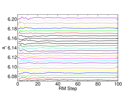
Figure 1: Determination of the $a_{i}$ coefficient along the Robbins Monro evolution for all the action intervals

For all the above observables we use the Madras-Sokal definition of the autocorrelation time Madras:1988ei , implemented according to Refs. Wolff:2003sm ; Luscher:2005rx . $\bar{\Gamma}(\xi)$ is the autocorrelation as function of the time lag $\xi$ between measurements:

$$\bar{\Gamma}(\xi)=\frac{1}{N-\xi}\sum_{i=1}^{N-\xi}\left(\mathcal{B}_{i}-\bar{\mathcal{B}}\right)\left(\mathcal{B}_{i+\xi}-\bar{\mathcal{B}}\right)\,,$$ (16)

where $N$ is total number of measurements, $\mathcal{B}_{i}$ denotes the i-th measurement of the observable $\mathcal{B}$, and $\bar{\mathcal{B}}$ its average. The integrated autocorrelation time $\tau_{\mathrm{int}}$ is defined as:

$$\tau_{\mathrm{int}}=\frac{1}{2}+\sum_{\xi=1}^{W}\bar{\Gamma}(\xi)/\bar{\Gamma}(0)\,,$$ (17)

where $W$ is the size of the Madras-Sokal window.

3.1 Tuning of the replica exchange method

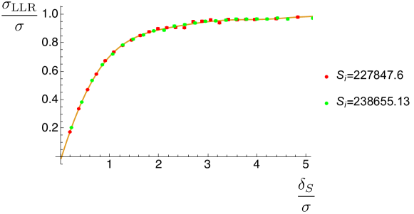
Figure 2: Behaviour of the variance of the constrained action versus the width of the support function normalized to the variance of the unconstrained action

The swapping probability of two replicas will depend on the size of their overlapping probability distributions, hence typically it will depend on $\mathcal{S}\>\!_{i}$ and on the fluctuation size of the constrained evolution $\sigma_{\rm LLR}=\sqrt{\left\langle\kern-1.69998pt\left\langle\mathcal{S}\>\!^{2}\right\rangle\kern-1.69998pt\right\rangle_{i}-\left\langle\kern-1.69998pt\left\langle\mathcal{S}\>\!\right\rangle\kern-1.69998pt\right\rangle^{2}_{i}}$. In order to tune the swapping probability among different replicas we noted that it is possible to relate the $\sigma_{\rm LLR}$ to the width of the support function ($\delta_{S}$) and to the variance of the unconstrained evolution $\sigma$ for identical action values. This study is reported in figure 2 where the asymptotic behaviour both for small $\delta_{S}$ ($\sigma\simeq\delta_{S}$) and large $\delta_{S}$ ($\sigma_{\rm LLR}\simeq\sigma$) can be clearly highlighted. An additional feature of this study is the independence within our numerical precision of the scaling function with respect to the central action value. Thanks to this feature, it becomes possible, with the only knowledge of the variance of the unconstrained action as function of $\beta$, to generate a sequence of $\mathcal{S}\>\!_{i}$ and $(\delta_{S})_{i}$ for which the overlapping spread of action among neighbouring replicas is equal. If we define the swap probability as the probability for fixed energy value to swap configurations with any other replica, it is possible to show that the tuning just described gives rise to a flat swap probability among all the replicas. By changing the size of the overlapping region it is possible to tune the swapping probability to the desired value, in figure 3 the case of probability $\sim 50\%$.

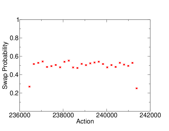
Figure 3: Swap probability as function of the central action

A final note is in order: the Markov Chain process defined in this way is still distributed according the detailed balance of energy when considering the whole set of replicas, as such the autocorrelation time can be measured only on the observables reweighed over all the replicas together and not on a single replica at a time.

4 Results

We have performed an extensive investigation of the properties of our algorithm and compared our findings against the results of traditional HMC simulations for all the observables described in sec.3, together with their autocorrelation times. For a rough cost budget we have generated $0.7\cdot 10^{5}$ configurations per replica and divided the action interval over 26 replicas, while for each traditional simulation we have generated $1.1\cdot 10^{5}$ configurations. We produced estimates of our observables only in an internal region defined such that the reweighed observables could have a contribution from the boundary $10^{-4}$ times smaller than the central contribution. All our estimates agree within the statistical error with their reference comparisons, and depending on the observables the statistical error associated with the observables measured with the LLR approach is at least a factor 2 smaller then traditional simulations. More importantly the autocorrelation time of all the investigated observables, once the replica exchange is taken into account, is smaller than the equivalent traditional simulation, signalling a good ergodicity property of the algorithm.

  

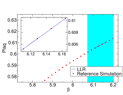
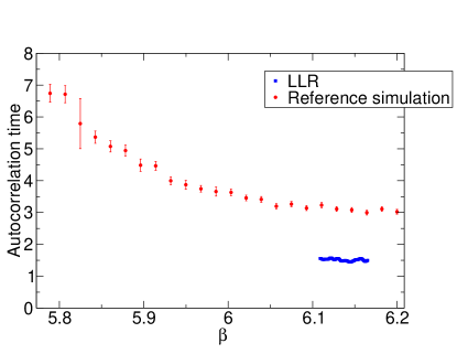
Figure 4: Plaquette and its autocorrelation time as function of $\beta$ at fixed lattice volume

  

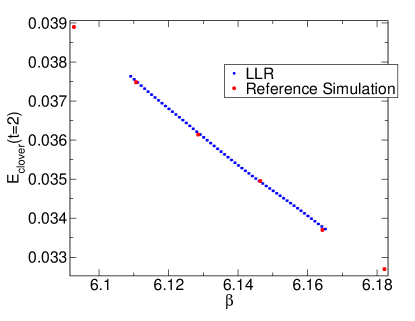
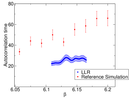
Figure 5: Clover energy at flow time $t=2$ and its autocorrelation time as function of $\beta$ at fixed lattice volume

  

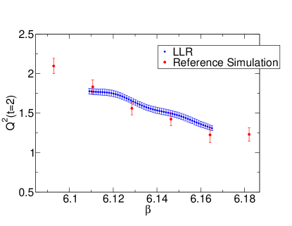
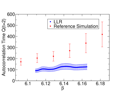
Figure 6: Topological susceptibility at flow time $t=2$ and the autocorrelation time of the topological charge as function of $\beta$ at fixed lattice volume

5 Conclusions

In this work we have investigated the ergodicity properties of the LLR method to evaluate the density of state. We focused in our study on the SU(3) pure Yang Mills theory, to test the behaviour of our method with theories that possess topological vacua. We measured observables sensitive to the topological structure alongside other less sensitive observables, and compared our findings with equivalent investigation done with traditional techniques. We have shown that the use of a replica exchange technique alleviates the problem of slow update dynamic evolution also in presence of the topological vacua. We have shown that the LLR method is capable of comparable precision in all the estimates at a comparable resource cost once the autocorrelation is taken into account. Simulation are still ongoing to investigate the scaling properties of this algorithm towards the continuum limit.

6 Acknowledgments

GC is supported by the STFC Consolidated Grant ST/L000458/1. BL is supported in part by the Royal Society and the Wolfson Foundation and the STFC Consolidated Grants ST/L000369/1 ST/P00055X/1. AR is supported by the STFC Consolidated Grants ST/L000350/1 and ST/P000479/1. The numerical computations have been carried out using resources from the HPCC Plymouth and the Supercomputing Wales (supported by the ERDF through the WEFO, which is part of the Welsh Government).

References

- (1) K. Langfeld, B. Lucini, A. Rago, Phys.Rev.Lett. 109, 111601 (2012), 1204.3243
- (2) K. Langfeld, B. Lucini, R. Pellegrini, A. Rago, Eur. Phys. J. C76, 306 (2016), 1509.08391
- (3) H. Robbins, S. Monro, Ann. Math. Statist. 22, 400 (1951)
- (4) R. Pellegrini, B. Lucini, A. Rago, D. Vadacchino, PoS LATTICE2016, 276 (2017)
- (5) B. Lucini, W. Fall, K. Langfeld, PoS LATTICE2016, 275 (2016), 1611.00019
- (6) S. Schaefer, R. Sommer, F. Virotta (ALPHA), Nucl. Phys. B845, 93 (2011), 1009.5228
- (7) M. LÃscher, JHEP 08, 071 (2010), [Erratum: JHEP03,092(2014)], 1006.4518
- (8) M. Luscher, S. Schaefer, JHEP 07, 036 (2011), 1105.4749
- (9) N. Madras, A.D. Sokal, J. Statist. Phys. 50, 109 (1988)
- (10) U. Wolff (ALPHA), Comput. Phys. Commun. 156, 143 (2004), [Erratum: Comput. Phys. Commun.176,383(2007)], hep-lat/0306017
- (11) M. Luscher, Comput. Phys. Commun. 165, 199 (2005), hep-lat/0409106