IFIC/17-45
Quasi-Dirac neutrino oscillations

Abstract

Dirac neutrino masses require two distinct neutral Weyl spinors per generation, with a special arrangement of masses and interactions with charged leptons. Once this arrangement is perturbed, lepton number is no longer conserved and neutrinos become Majorana particles. If these lepton number violating perturbations are small compared to the Dirac mass terms, neutrinos are quasi-Dirac particles. Alternatively, this scenario can be characterized by the existence of pairs of neutrinos with almost degenerate masses, and a lepton mixing matrix which has 12 angles and 12 phases. In this work we discuss the phenomenology of quasi-Dirac neutrino oscillations and derive limits on the relevant parameter space from various experiments. In one parameter perturbations of the Dirac limit, very stringent bounds can be derived on the mass splittings between the almost degenerate pairs of neutrinos. However, we also demonstrate that with suitable changes to the lepton mixing matrix, limits on such mass splittings are much weaker, or even completely absent. Finally, we consider the possibility that the mass splittings are too small to be measured and discuss bounds on the new, non-standard lepton mixing angles from current experiments for this case.

Keywords: Neutrinos, quasi-Dirac, pseudo-Dirac, Majorana, experimental constraints.

1 Introduction

Neutrino oscillation experiments cannot distinguish Dirac from Majorana neutrinos, hence it is still unknown whether or not lepton number is conserved. Other processes, such as neutrinoless double beta decay [1, 2], need to be probed in order to answer this question. However, while the nature of neutrinos is often seen as a dichotomy, presenting two sharply distinct scenarios, the Dirac neutrino case can be seen as a limit of the more general Majorana case in which lepton number violating mass terms are zero, and this limit can be approached smoothly.

In practice, one can start with a model of $2n$ Majorana neutrinos and get a phenomenology arbitrarily close to the one of a model of $n$ Dirac neutrinos. This can already be seen with only one generation of active ($\nu$) and sterile neutrinos ($N^{c}$). In the basis $\left(\nu,N^{c}\right)^{T}$ the most general mass matrix reads:

$$m_{\nu}=\left(\begin{array}[]{cc}m_{L}&m_{D}\\ m_{D}&m_{R}\end{array}\right)\,.$$ (1)

If $m_{L}=m_{R}=0$, lepton number is preserved and neutrinos are Dirac particles. This limit can alternatively be characterized by two exactly degenerate mass eigenstates composed in equal parts of $\nu$ and $N^{c}$: $\nu_{1}=1/\sqrt{2}\left(\nu+N^{c}\right)$ and $\nu_{2}=i/\sqrt{2}\left(-\nu+N^{c}\right)$. Small deviations from the limit $m_{L}=m_{R}=0$ lead to a quasi-Dirac scenario where lepton number is no longer exactly preserved.

Let us rewrite eq. (1) using:

$$\varepsilon=\frac{(m_{L}+m_{R})}{2m_{D}},$$ (2)

$$\theta=\frac{(m_{L}-m_{R})}{4m_{D}}.$$ (3)

As long as $\varepsilon$ and $\theta$ are much smaller than one, we obtain:

$$m_{1,2} \simeq m_{D}\left(1\pm\varepsilon\right)\,,$$ (4)

$$\nu_{1} \simeq 1/\sqrt{2}\left[\left(1+\theta\right)\nu+\left(1-\theta\right)N^{c}\right]\,,$$ (5)

$$\nu_{2} \simeq i/\sqrt{2}\left[\left(-1+\theta\right)\nu+\left(1+\theta\right)N^{c}\right]\,.$$ (6)

Departures from the Dirac case therefore can manifest themselves as either new mass splittings or new mixing angles (or, in general, both). Moreover, as this simple example shows, mass splittings and mixing angles are completely independent of each other. Note that for small values of $\varepsilon$ and $\theta$, lepton number violation is naturally suppressed, as expected. This can be most easily seen in our one generation scenario for the double beta decay observable $\langle m_{\nu}\rangle$: for $\theta=0$ ($\varepsilon=0$) it is straightforwardly calculated to be $\langle m_{\nu}\rangle\simeq\varepsilon m_{D}$ ($\langle m_{\nu}\rangle\simeq 2\theta m_{D}$).

We have therefore the following situation. Oscillation experiments cannot distinguish a model with $n$ Majorana neutrinos (containing $n$ Weyl spinors) from one with $n$ Dirac neutrinos (containing $2n$ Weyl spinors) with matching masses and mixing angles. Nevertheless, once we add to a model with Dirac neutrinos small sources of lepton number violation, oscillation probabilities will change. Some illustrative examples are shown in fig. (1). We plot there the electron neutrino survival probability for low-energy (reactor) neutrinos at distances up to (and slightly larger than) the typical distances of the KamLAND experiment [3]. In all plots the black lines show the expectation for the current global best fit point [4] for the ordinary neutrino parameters in the standard three generation case, to which we have added either a non-zero mass splitting to a Dirac state (top row) or one particular new quasi-Dirac angle (bottom row).

In section (2) we will discuss the general parametrization of masses and mixing angles for scenarios with three generations of quasi-Dirac neutrinos. However, from the examples shown in fig. (1) one can read off already some basic facts about oscillations of quasi-Dirac neutrinos, which we will work out in greater detail in section (3). First, small non-zero values of $\varepsilon$’s are equivalent to introducing new, large oscillation lengths. Thus, the best constraints on $\varepsilon$ will come from oscillation experiments with the largest possible baselines. And secondly, even if mass splittings are negligibly small, the new, non-standard angles which appear in this setup (called $\theta$ above) may affect oscillation probabilities in a way similar to standard angles, hence creating parameter degeneracies. For example, as fig. (1) shows, from $P_{ee}$ alone one cannot provide limits on a single angle. (In this example variations of $\theta_{14}$ can be compensated by varying $\theta_{12}$.) Even by combining more than one oscillation probability, constraints can only be derived for certain combinations of angles and phases of the mixing matrix. We will discuss this in detail in section (3.2). Constraints on mass splittings are discussed in section (3.1).

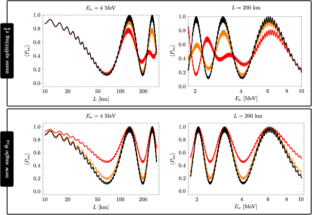
Figure 1: Electron neutrino survival probability for quasi-Dirac neutrinos with a fixed energy $E_{\nu}=4$ MeV as a function of distance (left), and for fixed distance $L=200$ km as function of $E_{\nu}$ (right). The standard 3-generation neutrino oscillation parameters have been fixed at their best fit point values [4], to which a small perturbation has been added. In the top row, we show the effect of mass splittings: $\varepsilon_{2}^{2}=0$ (black), $\varepsilon_{2}^{2}=10^{-5}$ eV² (orange) and $\varepsilon_{2}^{2}=2\times 10^{-5}$ eV² (red). In the bottom row, it is possible to see the effect of introducing a non-standard angle: $\theta_{14}=0$ (black), $\theta_{14}=\pi/8$ (orange) and $\theta_{14}=\pi/4$ (red). The exact definition of $\varepsilon_{2}$ and $\theta_{14}$ will be given latter in section (2).

A word on nomenclature. The terminologies quasi-Dirac and pseudo-Dirac neutrinos appear nearly interchangeably in the literature. We prefer to define quasi-Dirac (QD) neutrinos as being a mixture of active and sterile states, in contrast with pseudo-Dirac (PD) neutrinos which are composed of active states only. In both cases, the structure of mass and mixing matrices must be such that the lepton sector is close to preserving one or more $U(1)$ symmetries.

With this definition, quasi-Dirac and pseudo-Dirac neutrinos are then very different objects, both theoretically and phenomenologically. Let us briefly mention that various aspects of pseudo-Dirac neutrinos have been considered in the literature: Magnetic moments and double beta decay [7], possible mass textures [8, 9, 10], and oscillatory behavior [11, 12, 13, 14]. We note in passing that models of pseudo-Dirac neutrinos require neutrino mass matrices which no longer fit the solar and atmospheric neutrino oscillation data [15, 16, 17].

Many more papers discussed the phenomenology of quasi-Dirac neutrinos. For example, double beta decay was first discussed in this context in [6], while [19] and [20, 21] consider quasi-Dirac neutrinos as a possible explanation of the atmospheric and solar neutrino problems, respectively. More ambitiously, explaining atmospheric, solar and LSND neutrino oscillations simultaneously was discussed in [22, 23]. However, all these proposals are by now ruled out experimentally, since they predict too much oscillations into sterile neutrinos. Limits on quasi-Dirac neutrino parameters, on the other hand, have been derived from solar neutrino data [24] as well as from solar, atmospheric neutrino data and cosmology [25]. Furthermore, in [26, 27, 28, 29] QD neutrinos have been discussed in the context of neutrino telescopes, such as IceCube.

Quasi-Dirac neutrino oscillations were also discussed in [30], where it was claimed that to leading order in $m_{R,L}/m_{D}$ the flavor composition of the mass eigenstates does not change (only mass splittings appear), hence oscillations for $n=3$ pairs of quasi-Dirac neutrinos are described by the standard mixing matrix. This assertion was taken to be true by others [26, 27, 28, 31], yet we want to stress that this claim is not correct, as can be seen from the eqs. (4)–(6). Already for one generation, these expressions show that the mass splitting and the departure from maximal mixing are both linearly dependent on $m_{R,L}$ and, more importantly, they are controlled by orthogonal combinations of these two parameters. As such, it is even possible to have no mass splittings at all and at the same time have arbitrary mixing angles.

There are also a number of more theoretical papers discussing how quasi-Dirac neutrinos could arise. One possibility is the so-called “singular” seesaw where the mass matrix for the singlet neutrinos ($N^{c}$) has a determinant equal or close to zero [32]. Quasi-Dirac neutrinos from such a singular seesaw with additional type-II seesaw contributions have been discussed in [33]. Another possibility [31] involves introducing additional singlets ($S$), as it is done for the inverse seesaw mechanism [34]. A double seesaw is then responsible for producing very light $S$ states which, together with the active states, form quasi-Dirac neutrinos [31]. The authors of [35] use a Dirac seesaw to explain the necessary smallness of the Dirac neutrino mass terms first, and then generate quasi-Dirac states by the addition of a very small seesaw type-II term. The “mirror world” model of [36] is another way to obtain these particles.

In models with extended gauge groups quasi-Dirac neutrinos can also appear. An example is the $E_{6}$ inspired $331$ model of [37]. Here, several electroweak triplets of the gauge group $SU(3)_{L}$ are needed to accomodate the Standard Model leptons, and the observed active light neutrinos are automatically quasi-Dirac states [38]. A very different idea, based on supergravity has been discussed in [39]. There it was pointed out that if neutrino Dirac terms are generated from the Kähler potential (instead of the superpotential), neutrinos would be quasi-Dirac, since Majorana terms come from higher order Kähler potential terms and thus are expected to be suppressed. This idea [39] is particularly attractive, since it could, at least in principle, explain the observed smallness of the Dirac neutrino mass terms.

In addition to $n$ active neutrinos, models of Dirac neutrinos require the introduction of $n$ Weyl spinors transforming trivially under the electroweak gauge group. For this reason, the study of quasi-Dirac neutrinos necessarily has some overlap with the physics of sterile neutrinos. Many experiments have searched for sterile neutrinos. Most famously, the SNO neutral current measurement rules out dominant contributions of sterile neutrinos to the solar neutrino oscillations [40]. Super-Kamiokande searched for steriles in atmospheric neutrinos [41]. OPERA [42], MINOS and DayaBay [43], IceCube[44] and NO$\nu$A [45] published searches for sterile neutrinos. For a more complete list of references see the recent reviews [46, 47]. Note, however, that constraints on sterile are usually derived assuming best fit point values for the standard oscillation parameters, to which two new parameters (one angle and one mass splitting) are added in the fit. This approach does not cover the general quasi-Dirac neutrino parameter space. In particular, keeping the standard neutrino parameters fixed can lead to misleading conclusions about limits for the new/extra parameters.

There are also some hints for the existence of sterile neutrinos. However, all these hints point to a new and much larger mass scale in oscillations, i.e. $\Delta m^{2}\simeq{\cal O}$(1) eV². Since these indications imply masses and mixings very different from those of the standard oscillations, they can not be explained by quasi-Dirac neutrinos. We thus do not discuss these hints any further and refer only to the recent review [47].

The rest of this paper is organized as follows. In section (2) we discuss the basics of quasi-Dirac oscillations, constructing general expressions for the mixing matrix for the three generation case. In section (3) we discuss constraints on the new, non-standard parameters from various neutrino experiments. Constraints on quasi-Dirac mass splittings are discussed in section (3.1), while in section (3.2) we discuss the constraints on angles, for the case in which mass splittings are negligible. We then close with a short summary and discussion.

2 Definitions for quasi-Dirac neutrino oscillations

Dirac neutrinos can be described either in the weak or in the mass basis. The two pictures are equivalent. We will choose the latter one. Consider then a lepton-number preserving model with three active and three sterile neutrinos ($\nu$ and $N^{c}$). In the basis where the charged lepton mass matrix is diagonal, the relevant part of the Lagrangian reads

$$\mathscr{L} =\frac{g}{\sqrt{2}}\overline{\ell_{L}}\mathds{1}\gamma^{\mu}\nu W_{\mu}^{-}+\nu^{T}m_{\nu}N^{c}+\textrm{h.c.}\;\;\textrm{$\left[\textrm{flavor basis}\right]$}\,.$$ (7)

In order to diagonalize the matrix $m_{\nu}$, both active and sterile neutrinos must be rotated, $\nu\rightarrow V\nu$ and $N^{c}\rightarrow V_{N}N^{c}$, such that $m_{\nu}^{\textrm{(diag)}}=V^{T}m_{\nu}V_{N}$:

$$\mathscr{L} =\frac{g}{\sqrt{2}}\overline{\ell_{L}}V\gamma^{\mu}\nu W_{\mu}^{-}+\nu^{T}m_{\nu}^{\textrm{(diag)}}N^{c}+\textrm{h.c.}\;\;\textrm{$\left[\textrm{mass basis 1}\right]$}\,.$$ (8)

Strictly speaking, the neutrino mass matrix is not yet diagonal since it is still mixing different states (active and sterile neutrinos). This can be solved by rewriting $\nu_{i}$ and $N_{i}^{c}$ ($i=1,2,3$) as $\psi_{i}\equiv 1/\sqrt{2}\left(\nu_{i}+N_{i}^{c}\right)$, and $\psi_{i+3}\equiv i/\sqrt{2}\left(-\nu_{i}+N_{i}^{c}\right)$:

$$\mathscr{L} =\frac{g}{\sqrt{2}}\overline{\ell_{L}}\Omega\gamma^{\mu}\psi W_{\mu}^{-}+\sum_{j=1}^{6}m^{\psi}_{j}\psi_{j}\psi_{j}+\textrm{h.c.}\;\;\textrm{$\left[\textrm{mass basis 2}\right]$}\,.$$ (9)

where the masses and the $3\times 6$ mixing matrix $\Omega$ have a special form ($V$ is a $3\times 3$ square matrix):

$$m^{\psi}_{j} =\left(m_{1},m_{2},m_{3},m_{1},m_{2},m_{3}\right)\;\;\hskip 51.21504pt\textrm{$\left[\textrm{Dirac limit}\right]$}\,,$$ (10)

$$\Omega =\frac{1}{\sqrt{2}}\left[\begin{array}[]{ccc}\ddots&&\iddots\\ &V\\ \iddots&&\ddots\end{array},\begin{array}[]{ccc}\ddots&&\iddots\\ &iV\\ \iddots&&\ddots\end{array}\right]\;\;\textrm{$\left[\textrm{Dirac limit}\right]$}\,.$$ (17)

If the pattern of masses and mixing in eqs. (10) and (17) is perturbed, neutrinos are no longer Dirac particles and lepton number is violated. Note that this is equivalent to switching on the lepton number violating masses $m_{L}$ and $m_{R}$ in eq. (1). We shall now look into the possible departures from the Dirac limit as seen from the mass basis.

In the case of masses, it is possible to split the three pairs of $\left(m^{\psi}_{i},m^{\psi}_{i+3}\right)$, hence we may introduce three $\varepsilon_{i}$ such that

$$\left(m_{i}^{\psi}\right)^{2},\left(m_{i+3}^{\psi}\right)^{2} \rightarrow m_{i}^{2}-\frac{\varepsilon_{i}^{2}}{2},m_{i}^{2}+\frac{\varepsilon_{i}^{2}}{2}\,,$$ (18)

with the understanding that, for quasi-Dirac neutrinos, the $\varepsilon_{i}$ are small in comparison to the atmospheric and solar mass scales. In total there are now five mass parameters relevant for oscillation experiments: the usual $\Delta m^{2}_{\rm Atm}$ and $\Delta m^{2}_{\odot}$, plus three new $\varepsilon_{i}$ mass splittings. (As usual, the overall mass scale of neutrinos does not enter the oscillation probabilities.)

Let us now turn our attention to a generic mixing matrix $\Omega$ with dimensions $n\times m$. Such a matrix can be described by $2nm$ real numbers, yet orthonormality of rows ($\Omega\Omega^{\dagger}=\mathds{1}$) imposes $n^{2}$ conditions on them, and furthermore it is possible to absorb $n$ phases into the charged lepton fields, hence there is a total of $n\left(2m-n-1\right)$ real physical degrees of freedom in $\Omega$. For a $3\times 6$ matrix, this corresponds to 12 angles and 12 phases, but note that 5 of these phases cannot be observed in neutrino oscillation experiments (they correspond to column phases). The matrix $\Omega$ can be explicitly parametrized as follows [48] (called below the SV parametrization). First, consider an elementary rotation in the $\left(i,j\right)$ entries given by the complex number $\widetilde{\theta}_{ij}\equiv\theta_{ij}\exp i\phi_{ij}$ such that, in the (1,2) case, it has the form

$$R\left(\widetilde{\theta}_{12}\right) =\left(\begin{array}[]{cccc}\cos\theta_{12}&-e^{i\phi_{12}}\sin\theta_{12}&0&\cdots\\ e^{-i\phi_{12}}\sin\theta_{12}&\cos\theta_{12}&0&\cdots\\ 0&0&1&\cdots\\ \vdots&\vdots&\vdots&\ddots\end{array}\right)\,.$$ (23)

In the SV parametrization, the $i$-th row of $\Omega$ ($\equiv\Omega_{i}$) is then given by the expression

$$\Omega_{SV,i}^{T} =\prod_{a=1}^{i}\prod_{b=a+1}^{6}R\left(\widetilde{\theta}_{ab}\right)e^{(i)}\,,$$ (24)

where $e^{(i)}$ is a column vector with entries $e_{j}^{(i)}=\delta_{ij}$. We do not give here $\Omega_{SV}$ in full because the expression is very lengthy.

For a particular arrangement of the 24 angles and phases in eq. (24), $\Omega$ takes the special form (17) which is associated with the Dirac limit. Note that, as usual, one can write the $3\times 3$ square matrix $V$ with three angles and one phase:

$$V =\left(\begin{array}[]{ccc}1&0&0\\ 0&\cos\theta_{23}&\sin\theta_{23}\\ 0&-\sin\theta_{23}&\cos\theta_{23}\end{array}\right)\left(\begin{array}[]{ccc}\cos\theta_{13}&0&\sin\theta_{13}e^{-i\delta}\\ 0&1&0\\ -\sin\theta_{13}e^{i\delta}&0&\cos\theta_{13}\end{array}\right)\left(\begin{array}[]{ccc}\cos\theta_{12}&\sin\theta_{12}&0\\ -\sin\theta_{12}&\cos\theta_{12}&0\\ 0&0&1\end{array}\right)\,.$$ (34)

Unfortunately, it is very complicated to describe the Dirac limit in the SV parametrization. Hence we make a small modification by introducing the following $6\times 6$ rotation matrix:

$$\Omega\left(\theta_{ij},\phi_{ij}\right) \equiv\Omega_{SV}\left(\theta_{ij},\phi_{ij}\right)U\;,\,U=\frac{1}{\sqrt{2}}\left(\begin{array}[]{cc}\mathbb{1}&i\mathbb{1}\\ \mathbb{1}&-i\mathbb{1}\end{array}\right)\,.$$ (37)

With this definition, the mixing matrix in eq. (17), with $V$ parametrized as in eq. (34), corresponds to $\Omega\left(\theta_{ij},\phi_{ij}\right)$, as in (37), with $\theta_{i4}=\theta_{i5}=\theta_{i6}=0$ ($i=1,2,3$), $\phi_{12}=\phi_{23}=0$ and $\phi_{13}=\delta$. In other words, with this definition the Dirac limit for $\Omega$ simply corresponds to keeping only the standard three generation neutrino mixing angles non-zero.

We can then write the probability of neutrino oscillation from a flavor $\alpha$ to a flavor $\beta$ for an energy $E$ and after a length $L$ as:

$$P\left(\nu_{\alpha}\rightarrow\nu_{\beta}\right) =\left|\sum_{j=1}^{6}\Omega_{\beta j}\Omega_{\alpha j}^{*}\exp\left(-\frac{im_{j}^{2}L}{2E}\right)\right|^{2}$$ (38)

Note that this expression is insensitive to column rephasings $\Omega\rightarrow\Omega\,\textrm{diag}\left(e^{i\kappa_{1}},e^{i\kappa_{2}},e^{i\kappa_{3}},e^{i\kappa_{4}},e^{i\kappa_{5}},e^{i\kappa_{6}}\right)$. It is easy to show that eq. (38) reduces to the standard oscillation formula in the Dirac limit.

3 Current experimental limits and future prospects

As discussed in the previous section, the full parameter space for a system of 3 pairs of QD neutrinos has 30 free parameters: Two independent $\Delta m_{ij}^{2}$ plus one overall mass scale, three $\varepsilon_{i}^{2}$, twelve angles and twelve phases. Even discounting the five Majorana phases and the overall mass scale, which can not be probed in oscillation experiments, the remaining number of parameters is much too large to fit simultaneously.

Nearly all experimental data, on the other hand, is consistent with the standard picture of only three active neutrino species participating in oscillations [4], i.e. two mass squared differences ($\Delta m^{2}_{\rm Atm}$ and $\Delta m^{2}_{\odot}$), three mixing angles ($\theta_{23}$, $\theta_{12}$ and $\theta_{13}$) plus one phase ($\delta$) are sufficient to describe the data. As mentioned in the introduction, there are also some hints for sterile neutrinos with a mass scale of the order of $\Delta m^{2}\sim{\cal O}$(eV) [46, 47]. However, all these hints are at most of the order of ($2-3$) $\sigma$, we will thus not take them into account in the following. Instead, since the standard three generation picture seems to describe the data well, we will consider “small” perturbations and derive limits on particular combinations of non-standard parameters.

In order to deal effectively with the large number of parameters controlling quasi-Dirac neutrino oscillations, we will consider two simplified scenarios:

1. First, we take one non-zero $\varepsilon_{i}$ at a time. In these one-parameter extensions, very stringent limits on $\varepsilon_{i}$ are found, in agreement with earlier analysis, see for example [24, 25]. We then extend this analysis to two new parameters: One mass splitting plus one new angle. This second step allows us to identify “blind spots” in the oscillation experiments, i.e. degenerate minima in particular directions in parameter space, where limits on mass splittings are much worse than in the one parameter fits. We then discuss a particular parametrization of these degenerate directions in parameter space, where the effects of $\varepsilon_{i}$ can be decoupled from oscillation experiments nearly completely.

2. In the second setup, we discuss the limit where mass splittings are too small to be measured in oscillation experiments, hence there are just angles and phases of $\Omega$ to deal with. In this situation, it can be shown that from the 24 parameters in $\Omega$ only 13 combinations enter the oscillation probabilities of active neutrinos. Moreover, since there is only very limited information on oscillations involving $\nu_{\tau}$, we can in practice restrict ourselves to experiments involving $\nu_{e}$’s and $\nu_{\mu}$’s. There are then only 7 combinations of the 24 angles $\theta_{ij}$ and phases $\phi_{ij}$ which appear in the oscillation probabilities. We discuss the construction of these 7 quantities, the current constraints and possible tests for quasi-Dirac neutrinos in this limit.

In our analysis we do not take into account the data from every existing oscillation experiment. Given the scarcity of data on $\tau$ neutrinos, we ignored it altogether, concentrating instead on the available charged current data for $e$ and $\mu$ neutrinos and anti-neutrinos. Also, we focus on those experiments, which should provide the most important constraints for quasi-Dirac neutrinos. First, we consider KamLAND [3] since it fixes most accurately the so-called solar mass splitting $\Delta m^{2}_{\odot}$. From the solar neutrino experiments we fit Super-K elastic scattering data [49] and from Borexino the measured $pp$ [50] and ${}^{7}Be$ fluxes [51]. This choice is motivated by the fact that Super-K [49] has the most accurate data in the high energy range, while [50, 51] fix the low energy part of the solar neutrino spectrum.

We take the atmospheric neutrino data from [52]. We concentrate in our fit on the sub-GeV sample, since the lowest energetic neutrinos will be most sensitive to small values of $\varepsilon_{i}^{2}$, as demonstrated in fig. (2). In addition, we use data from the MINOS collaboration (muon and anti-muon neutrino survival) [53] and T2K (muon neutrino survival and muon to electron neutrino transition) [54], since these two experiments determine $\Delta m^{2}_{\rm Atm}$ better than atmospheric data. And, finally, we take into account data from DayaBay [55], since from the three current reactor neutrino experiments DayaBay determines $\theta_{13}$ with the smallest error.

Figure 2: Averaged atmospheric muon neutrino survival probability for neutrinos with energies $E_{\nu}=(0.1-1)$ GeV (left) and $E_{\nu}=(1-5)$ GeV (right), as a function of distance ($L$), for different choices of $\varepsilon_{3}^{2}$. Lower neutrino energies are more sensitive to small $\varepsilon_{3}$ values. This plot is calculated with the simplifying assumptions of $\sin^{2}\theta_{23}=1/2$, $\theta_{13}=0$ and $\Delta m^{2}_{\odot}=0$.

In our fits, we use a simple $\chi^{2}$ method to determine the allowed ranges of model parameters. We take statistical and systematic errors from the experimental publications, to which we added a further (small) systematic error for the uncertainties in our theoretical calculations. This latter systematic error was chosen such that our simulations reproduce the allowed parameter ranges for the standard oscillation parameters, determined by the respective experiment, within typically (1-1.5) $\sigma$ c.l. ranges. Note that we do not attempt to do a precision global fit for standard neutrino oscillation parameters. Rather, we consider reproducing the experimental results for the standard case as a test for the reliability of our derived limits.

3.1 Limits on mass splittings $\varepsilon_{i}$

3.1.1 One parameter limits

We will first discuss limits derived on $\varepsilon_{i}$ assuming one $\varepsilon_{i}\neq 0$ at a time and taking all non-standard angles to be zero. Table (1) shows limits on $\varepsilon_{i}^{2}$ and the corresponding experimental data sets used to derive the limits.

Experiment	$\varepsilon_{1}^{2}$ [eV2]	$\varepsilon_{2}^{2}$ [eV2]	$\varepsilon_{3}^{2}$ [eV2]
KamLAND	$7.7(3.4)\times 10^{-6}$	$1.7(1.0)\times 10^{-5}$	–
Solar + KamLAND	$1.7(1.3)\times 10^{-11}$	$1.7(1.5)\times 10^{-11}$	–
DayaBay + MINOS + T2K	–	$1.5(0.9)\times 10^{-4}$	$1.3(0.074)\times 10^{-3}$
Super-K + DayaBay + MINOS + T2K	–	$1.9(1.8)\times 10^{-5}$	$1.2(1.1)\times 10^{-5}$
JUNO	$1.7(0.07)\times 10^{-5}$	$2.3(0.09)\times 10^{-5}$	$6.0(2.2)\times 10^{-5}$

Table 1: 95 % upper limits on $\varepsilon_{i}^{2}$ derived from different experimental data sets. Two numbers are given for each case; the first one is the limit obtained marginalizing over two standard oscillation parameters (see text), the second (in brackets) is the limit obtained for the best fit point value of the standard oscillation parameters. For a discussion see text.

For each case listed in table (1), we have calculated the upper limits on the $\varepsilon_{i}^{2}$ twice: (a) marginalizing over two of the standard neutrino oscillation parameters and (b) for the best fit point value of the standard parameters. Marginalization over standard oscillation parameters leads to less stringent limits. However, the importance of this marginalization procedure differs widely for different experiments. For example, in the case of KamLAND, bounds on $\varepsilon_{1}^{2}$ of the order of roughly $10^{-5}$ are derived marginalizing over the allowed ranges of $\Delta m^{2}_{\odot}$ and $\sin^{2}\theta_{12}$, while for the best fit values of these last two parameters, the limits are more stringent by “only” roughly a factor 2.

As the table shows, the strongest constraints on $\varepsilon_{1}^{2}$ and $\varepsilon_{2}^{2}$ come from solar neutrino data. This is easily understood from fig. (3), which shows the electron neutrino survival probability as a function of neutrino energy for different values of $\varepsilon_{2}^{2}$ and for the best fit values of the standard solar oscillation parameters. For low values of neutrino energies, vacuum oscillations dominate and so very small $\varepsilon_{2}^{2}$ can be probed up to a scale essentially determined by the Earth-Sun distance ($\sim 10^{-12,-11}\textrm{ eV}^{2}$). Note that a non-zero $\varepsilon_{2}^{2}$ reduces $P_{ee}$, but this reduction could be hidden in the relatively large error bar of the low-energy measurements. Nevertheless, at higher neutrino energies, a similar reduction of $P_{ee}$ is produced due to matter effects in the sun. Since Super-K data provides a very accurate measurement of $P_{ee}$ at these higher energies, one can rule out values of $\varepsilon_{2}^{2}$ which can not be excluded by the Borexino measurements alone. The situation is very similar for $\varepsilon_{1}^{2}$: limits on $\varepsilon_{1}^{2}$ and $\varepsilon_{2}^{2}$ are then of the order of $10^{-11}$ eV² if we take the best fit values of the standard solar oscillation parameters; slightly less stringent numbers are obtained when marginalizing over the standard parameter uncertainties.

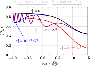
Figure 3: Solar neutrino survival probability as a function of neutrino energy, for different choices of $\varepsilon_{2}^{2}$. Solar angle and mass splitting have been fixed at their best fit values in this plot [4].

Solar neutrino experiments have essentially no sensitivity to $\varepsilon_{3}^{2}$. This is simply due to the smallness of $\theta_{13}$ ($\sin^{2}\theta_{13}\simeq 0.0215$ [4]). Thus, we have to rely on experiments testing the atmospheric scale to derive limits on $\varepsilon_{3}^{2}$. Table (1) quotes numbers for two cases.

In the first scenario, we have combined data from DayaBay [55], T2K [54] and MINOS [53]: DayaBay fixes most accurately $\theta_{13}$, while both MINOS and T2K measure $\Delta m^{2}_{\rm Atm}$ with rather small errors. Here, the limit on $\varepsilon_{2}^{2}$ is (not surprisingly) less stringent than the one derived from KamLAND (or solar). Depending on whether or not $\Delta m^{2}_{\rm Atm}$ and $\sin^{2}\theta_{\rm 23}$ are used at their best fit value or marginalized over, we get very different limits on $\varepsilon_{3}^{2}$. This is due to the fact that when scanning over the standard oscillation parameters, the $\chi^{2}$ function has two almost degenerate minima: one for small values of $\varepsilon_{3}^{2}$ and another for $\varepsilon_{3}^{2}$ of the order $10^{-3}$ eV². However, as the table also shows (second case), this non-standard solution is excluded, once we add Super-K atmospheric neutrino sub-GeV data to the fit. With the combination of these four experiments limits on $\varepsilon_{2}^{2}$ and $\varepsilon_{3}^{2}$ are again of order $10^{-5}$ eV².

In the last line of table (1) we give our forecast of the sensitivity of the planned experiment JUNO [56]. JUNO will measure $\Delta m^{2}_{\odot}$ and $\Delta m^{2}_{\rm Atm}$ very precisely and thus it will also be able to derive limits on any $\varepsilon_{i}^{2}$. However, our results indicate that, despite being a very precise experiment, JUNO will not lead to a major improvement over existing limits on $\varepsilon_{i}^{2}$. Here, it is important to stress that limits using the best fit point and limits marginalizing over standard parameter uncertainties are very different. This can be traced back again to a near-degeneracy in the $\chi^{2}$-function: For $\epsilon_{i}^{2}$ of the order of $\Delta m^{2}_{ij}$ one has two only slightly different oscillation lengths contributing in the fit, which can give a better description than a single oscillation length.

In summary, strong limits on mass splittings can be derived from atmospheric and solar neutrino data ($\varepsilon_{3}^{2}\sim{\cal O}(10^{-5})$ eV² and $\varepsilon_{1,2}^{2}\sim{\cal O}(10^{-11})$ eV², respectively) in the case where no other extra parameter is added to the standard neutrino oscillation picture.

3.1.2 Two parameter case

While the discussion in the previous subsection seems to show that constraints on QD mass splittings are very stringent, we will now see that this conclusion is valid only under the assumption that no other non-standard parameter is different from zero.

As a simple example, consider the electron neutrino survival probability at distances short enough that the effects of $\Delta m^{2}_{\odot}$ can be neglected. We shall consider the particular example of a non-zero $\varepsilon_{3}^{2}$ and a non-zero $\theta_{16}$ angle, defined in section 2. One finds that

$$P_{ee}=1-2c_{13}^{2}c_{16}^{2}\Big{(}\Delta m_{ee}^{-}(s_{16}+c_{16}s_{13})^{2}+\Delta m_{ee}^{+}(s_{16}-c_{16}s_{13})^{2}\Big{)}\,,$$ (39)

where $c_{ij}$ and $s_{ij}$ are short-hands for $\cos\theta_{ij}$ and $\sin\theta_{ij}$ and

$$\Delta m_{ee}^{\pm}\equiv c_{12}^{2}\sin^{2}\left[\frac{L}{4E}\left(\Delta m_{31}^{2}\pm\varepsilon_{3}^{2}/2\right)\right]+s_{12}^{2}\sin^{2}\left[\frac{L}{4E}\left(\Delta m_{32}^{2}\pm\varepsilon_{3}^{2}/2\right)\right]\,.$$ (40)

It is straightforward to see that the above expression for the neutrino survival probability remains (nearly) unchanged if we swap $\theta_{13}$ by $\theta_{16}$. This is true up to very small terms proportional to $\Delta(P_{ee})\propto(\Delta m_{ee}^{-}-\Delta m_{ee}^{+})(c_{13}-c_{16})s_{13}s_{16}$. More specifically, in the limit where $\Delta m_{ee}^{\pm}$ have the same value, $P_{ee}$ is only a function of the combination $\sin^{2}\theta_{13}+\sin^{2}\theta_{16}$. Thus, there will be a near-degeneracy of the relevant $\chi^{2}$ function involving these two angles, and so values (or limits) derived for one of these parameters, without varying the other, will be misleading.

There is, however, another more interesting degeneracy associated to eq. (39). In calculating this expression we have used a certain parametrization for the mass splitting, which we may call the symmetric parametrization: $m_{i},m_{i+3}\to\sqrt{m_{i}^{2}-\varepsilon_{i}^{2}/2},\sqrt{m_{i}^{2}+\varepsilon_{i}^{2}/2}$. Choosing $\sin\theta_{13}=\tan\theta_{16}$, the second term inside the bracket in eq. (39) vanishes (this choice corresponds to $\Omega_{e6}=0$). So, by adjusting $\Delta m^{2}_{31}$ and $\varepsilon_{3}^{2}$ we can keep $\Delta m^{2}_{31}-\varepsilon_{3}^{2}/2$ constant and equal to the best fit point value of $\Delta m^{2}_{\rm Atm}$, in which case there will be no upper limit on $\varepsilon_{3}^{2}$ itself coming from the electron neutrino survival experiments.

Note that we could have defined $m_{i},m_{i+3}\to m_{i},\sqrt{m_{i}^{2}+\varepsilon_{i}^{2}}$. We call this the asymmetric parametrization. Rewriting eq. (39) with this parametrization, the first term inside the bracket would not depend on $\varepsilon_{3}^{2}$ at all, so it becomes obvious that for the choice of $\sin\theta_{13}=\tan\theta_{16}$ all dependence of $P_{ee}$ on $\varepsilon_{3}^{2}$ disappears. Fig. (4) shows these parameter degeneracies in the space ($\varepsilon_{3}^{2},\sin^{2}\theta_{13},\sin^{2}\theta_{16}$), using only the DayaBay data (on the left column). The underlying scan was done in the asymmetric parametrization, which is numerically simpler to implement. The plot in the upper and middle panel show clearly that there is no upper limit on $\varepsilon_{3}^{2}$ in this scan. The lower plot shows the degeneracy in parameter space under the exchange of $\theta_{13}\leftrightarrow\theta_{16}$.

Figure 4: Allowed parameter ranges for $\varepsilon_{3}^{2}$, $\sin^{2}\theta_{13}$ and $\sin^{2}\theta_{16}$ for different experiments. The parameter planes always marginalize over the parameter not shown and all calculations used the best fit point value for $\Delta m^{2}_{\rm Atm}$. In the plots on the left only DayaBay data is taken into account; the middle panel combines DayaBay with T2K and the panel to the right shows the combination of DayaBay, T2K with Super-K atmospheric neutrino data. The different coloured regions present the 1, 2 and 3 $\sigma$ c.l. allowed regions (cyan, blue and red). For discussion see text.

We can break this particular degeneracy in parameter space, by adding more experiments. T2K measures two probabilities: (a) The muon neutrino survival probability, $P_{\mu\mu}$, and (b) the electron neutrino appearance probability, $P_{\mu e}$, both at values of $L/E$ which give access to the atmospheric neutrino mass scale, $\Delta m^{2}_{\rm Atm}$. If the only non-standard angle different from zero is $\theta_{16}$, then $P_{\mu\mu}$ will not depend on $\theta_{16}$ at all, while $P_{\mu e}$ will have $\theta_{16}$-dependence which is different from the one of $P_{ee}$. Thus, adding T2K data to the scan is enough to break the degeneracy in $\theta_{13}\leftrightarrow\theta_{16}$ hence an upper limit on $\varepsilon_{3}^{2}$ reappears. The middle column of fig. (4) illustrates this point; it shows the results of a combined scan over $\varepsilon_{3}^{2}$, $\sin^{2}\theta_{13}$ and $\sin^{2}\theta_{16}$ for DayaBay plus T2K data. By comparison of the right with the middle column of fig. (4), one can clearly see that the addition of Super-K data generates a strong upper limit on $\varepsilon_{3}^{2}$, for this particular choice of parameter subspace.

Given these results, one might wonder if there are particular directions in parameter space for which oscillation experiments become completely blind to QD neutrino mass splittings. Recall that the blind (or: degenerate) direction discussed above for $P_{ee}$ corresponds to the particular choice of $\Omega_{e6}=0$. In a similar way, for example, $P_{\mu\mu}$ would loose any sensitivity to $\varepsilon_{3}^{2}$ if $\Omega_{\mu 6}=0$. Thus, with some special choice of $\theta_{16}$ and $\theta_{26}$ such that both $\Omega_{e6}$ and $\Omega_{\mu 6}$ are zero at the same time, one can indeed make DayaBay and T2K blind to variations of $\varepsilon_{3}^{2}$.

While it is possible, in principle, to calculate the combination of angles $\theta_{ij}$ and phases $\phi_{ij}$ (defined in section (2)) associated to these blind directions, in the following we will consider a simpler alternative. Consider a unitary rotation of the columns $i$ and $i+3$ of the mixing matrix $\Omega$. Since we are not interested in column phases, such a rotation is governed by just two parameters ($\varphi_{i}$ and $\beta_{i}$):

$$\left(\begin{array}[]{cc}\vdots&\vdots\\ \rotatebox{90.0}{\;\;\;col. $i$ of $\Omega$}&\rotatebox{90.0}{col. $i+3$ of $\Omega$\;}\\ \vdots&\vdots\end{array}\right) \rightarrow\left(\begin{array}[]{cc}\vdots&\vdots\\ \rotatebox{90.0}{\;\;\;col. $i$ of $\Omega$}&\rotatebox{90.0}{col. $i+3$ of $\Omega$\;}\\ \vdots&\vdots\end{array}\right)\left(\begin{array}[]{cc}\cos\varphi_{i}&e^{i\beta_{i}}\sin\varphi_{i}\\ -e^{-i\beta_{i}}\sin\varphi_{i}&\cos\varphi_{i}\end{array}\right)$$ (49)

Now, recall that in the Dirac limit (see eq. (17)) the columns $i$ and $i+3$ of the mixing matrix $\Omega$ are proportional to each other, $\Omega_{\alpha,i}=-i\Omega_{\alpha,i+3}=V_{\alpha,i}/\sqrt{2}$. This means that applying the $\left(\varphi_{i},\beta_{i}\right)$ transformation to the Dirac neutrino mixing matrix and, without loss of generality setting $\beta_{i}=0$, we obtain:

$$\left(\begin{array}[]{cc}\vdots&\vdots\\ \Omega_{\alpha,i}&\Omega_{\alpha,i+3}\\ \vdots&\vdots\end{array}\right) =\left(\begin{array}[]{cc}\vdots&\vdots\\ \frac{\cos\varphi_{i}+\sin\varphi_{i}}{\sqrt{2}}V_{\alpha,i}&i\frac{\cos\varphi_{i}-\sin\varphi_{i}}{\sqrt{2}}V_{\alpha,i}\\ \vdots&\vdots\end{array}\right)\,.$$ (56)

From the last of these equations it can be seen that the $i$’th column (the ($i+3$)’th column) of $\Omega$ vanishes, if one chooses $\varphi_{i}=3\pi/4$ ($\varphi_{i}=\pi/4$).

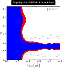
Figure 5: Allowed parameter space in the plane ($\varepsilon_{3}^{2},\varphi_{3}$) using DayaBay, T2K, MINOS and Super-K atmosheric neutrino data. The coloured plane shows the 2 and 3 $\sigma$ c.l. allowed regions (blue and red). The dashed lines show the expected limits for JUNO. The asymmetric parametrization of the mass splitting ($m_{3},\sqrt{m_{3}^{2}+\varepsilon_{3}^{2}}$) was used, so for $\varphi_{3}=\pi/4$ there is no sensitivity to $\varepsilon_{3}^{2}$.

Fig. (5) shows a scan over the allowed parameter space in the plane ($\varepsilon_{3}^{2},\varphi_{3}$) using DayaBay, T2K, MINOS and Super-K atmospheric neutrino data. In agreement with the above discussion, there is a blind spot where no limit on $\varepsilon_{3}^{2}$ exist. This blind direction corresponds to the choice of $\varphi_{3}=\pi/4$. Fig. (5) also shows that the addition of JUNO data can lead only to a marginally improved limit.

We now turn to a discussion of $\varepsilon_{1}^{2}$ and $\varepsilon_{2}^{2}$. For these two parameters, again solar neutrino physics provides the most important constraints. As above for $\varepsilon_{3}^{2}$, we can define a rotation angle $\varphi_{1}$ ($\varphi_{2}$) between the columns 1 and 4 (2 and 5) of the mixing angle which will mitigate the effects of a non-zero $\varepsilon_{1}^{2}$ ($\varepsilon_{2}^{2}$). Fig. (6) shows the $P_{ee}$ probability for solar neutrinos as a function of neutrino energy for two different values of $\varepsilon_{2}^{2}$ and various values of $\varphi_{2}$. The results for $\varepsilon_{1}^{2}$ and $\varphi_{1}$ are completely analogous. As the figure shows, for $\varphi_{2}=\pi/4$ again the effects of $\varepsilon_{2}^{2}$ completely decouple from the oscillation probability.

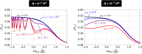
Figure 6: Average solar neutrino survival probability as a function of neutrino energy, for different choices of $\varphi_{2}$ and two different values of $\varepsilon_{2}^{2}$ and $\varphi_{2}$.

Fig. (7) shows the allowed parameter space in the two planes ($\varphi_{1},\varepsilon_{1}^{2}$) and ($\varphi_{2},\varepsilon_{2}^{2}$) using solar data and combining solar data with KamLAND. These plots have been calculated using the best fit point values for $\Delta m^{2}_{\odot}$ and $\sin^{2}\theta_{12}$ from the global fit [4]. The plots show in all cases that there exists a slight preference, between (2-2.5) $\sigma$ in all cases, for non-zero values of $\varepsilon_{i}^{2}$. Note that the preferred solution of the solar data in the region of $\varphi_{1}\sim 3/4\pi$ and $\varepsilon_{1}^{2}\sim(10^{-4.5}-10^{-4})$ is ruled out by KamLAND. However, even combining solar and KamLAND data some preference for non-zero $\varepsilon_{i}^{2}$ of the order of very roughly $10^{-10.5}$ eV² remains.

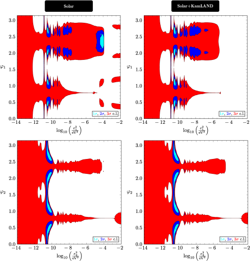
Figure 7: Allowed parameter range in the space $\varphi_{1},\varepsilon_{1}^{2}$ (top) and $\varphi_{2},\varepsilon_{2}^{2}$ (bottom). To the left: Solar data, to the right solar data + KamLAND. This plot uses the best fit point values for $\Delta m^{2}_{\odot}$ and $\sin^{2}\theta_{12}$ from the global fit. This combination of data shows a slight preference for a non-zero value of the mass splitting, for a discussion see text.

We have traced back this preference for non-zero mass splittings in solar data to the well-known difference in the best fit points from $\Delta m^{2}_{\odot}$ in solar and KamLAND data. As can be seen also in the latest global fits [4], solar data prefers a $\Delta m^{2}_{\odot}$ around $(4-5)\times 10^{-5}$ eV², while KamLAND prefers $\Delta m^{2}_{\odot}\simeq 7.6\times 10^{-5}$ eV². This tension between the two data sets is roughly of the order of 2 $\sigma$, with the error bar dominated by the larger error on $\Delta m^{2}_{\odot}$ in the solar data set. We have therefore recalculated the constraints on ($\varphi_{1},\varepsilon_{1}^{2}$) from solar data for a value of $\Delta m^{2}_{\odot}=4\times 10^{-5}$ eV². Fig. (8) shows the results of such a scan. As can be seen, in this calculation there is no longer any preference for a non-zero value of $\varepsilon_{1}^{2}$.

Note that such a low value of $\Delta m^{2}_{\odot}$ is ruled out by many $\sigma$ from the KamLAND data. Thus, a small non-zero mass splitting could provide, in principle, a solution for the observed tension between solar and KamLAND data.

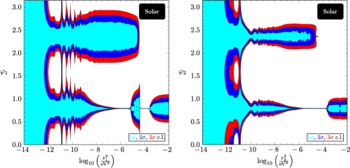
Figure 8: Allowed parameter range in the space $\varphi_{1},\varepsilon_{1}^{2}$ (left) and $\varphi_{2},\varepsilon_{2}^{2}$ (right) from solar data, using $\Delta m^{2}_{\odot}=4\times 10^{-5}$ eV².

In summary, by introducing one mass splitting at a time, we extracted bounds for the pairs of parameters $\left(\varepsilon_{i},\varphi_{i}\right)$, $i=1,2,3$. In the limit where $\varphi_{i}$ is $\left(2\pm 1\right)/4\pi$, one column of the mixing matrix vanishes and therefore the mass splitting $\varepsilon_{i}$ becomes unobservable. For this reason, one expects that for reasonably large values of $\varepsilon_{i}$ there must be tight limits on $\left|\varphi_{i}-\left(2\pm 1\right)/4\pi\right|$, meaning that $\varphi_{i}$ has to be quite far from the Dirac limit ($\varphi_{i}=0$). On the other hand, for a small enough value of the mass splitting $\varepsilon_{i}$, the associated oscillation length eventually become larger than the baseline of the relevant experiments, and in that case $\varphi_{i}$ becomes unconstrained.

3.2 Quasi-Dirac neutrinos in the limit $\varepsilon_{i}\to 0$

If masses are degenerate as in eq. (10), then the oscillation probability formula will not change under unitary rotations of the columns $i$ and $i+3$ of the mixing matrix, see eq. (49). In other words,

$$\left(\begin{array}[]{cc}\vdots&\vdots\\ \rotatebox{90.0}{\;\;\;col. $i$ of $\Omega$}&\rotatebox{90.0}{col. $i+3$ of $\Omega$\;}\\ \vdots&\vdots\end{array}\right) \rightarrow\left(\begin{array}[]{cc}\vdots&\vdots\\ \rotatebox{90.0}{\;\;\;col. $i$ of $\Omega$}&\rotatebox{90.0}{col. $i+3$ of $\Omega$\;}\\ \vdots&\vdots\end{array}\right)U(i)$$ (63)

for unitary matrices $U(i)$ ($i=1,2,3$) leaves $P\left(\nu_{\alpha}\rightarrow\nu_{\beta}\right)$ unchanged. Hence, there is a $U(2)^{3}$ redundancy in our description of $\Omega$, and in turn this means that out of the 24 parameters describing the mixing matrix, oscillation experiments are only sensitive to 13. This number is further reduced to 7 if we ignore tau neutrinos. In this latter case the oscillation probabilities can be written as:

$$P\left(\nu_{e}\rightarrow\nu_{e}\right) =1+\left(1-X_{1}-X_{2}\right)X_{2}\mathcal{A}_{12}+\left(1-X_{1}-X_{2}\right)X_{1}\mathcal{A}_{13}+X_{1}X_{2}\mathcal{A}_{23}\,,$$ (64)

$$P\left(\nu_{\mu}\rightarrow\nu_{\mu}\right) =1+\left(1-X_{3}-X_{4}\right)X_{4}\mathcal{A}_{12}+\left(1-X_{3}-X_{4}\right)X_{3}\mathcal{A}_{13}+X_{3}X_{4}\mathcal{A}_{23}\,,$$ (65)

$$P\left(\nu_{e}\rightarrow\nu_{\mu}\right) =-\left(X_{6}+\textrm{Re}X_{7}\right)\mathcal{A}_{12}-\left(X_{5}+\textrm{Re}X_{7}\right)\mathcal{A}_{13}+\textrm{Re}X_{7}\mathcal{A}_{23}+\textrm{Im}X_{7}\left(\mathcal{B}_{12}-\mathcal{B}_{13}+\mathcal{B}_{23}\right)\,,$$ (66)

with the oscillating factors $\mathcal{A}_{ij}\equiv-4\sin^{2}\left[\left(m_{i}^{2}-m_{j}^{2}\right)L/\left(4E\right)\right]$ and $\mathcal{B}_{ij}\equiv 2\sin\left[\left(m_{i}^{2}-m_{j}^{2}\right)L/\left(2E\right)\right]$ and the 7 parameters $X_{i}$ defined as follows:

$$X_{1}\equiv\left|\Omega_{e3}\right|^{2}+\left|\Omega_{e6}\right|^{2}\,,\,X_{2}\equiv\left|\Omega_{e2}\right|^{2}+\left|\Omega_{e5}\right|^{2}\,,$$ (67)

$$X_{3}\equiv\left|\Omega_{\mu 3}\right|^{2}+\left|\Omega_{\mu 6}\right|^{2}\,,\,X_{4}\equiv\left|\Omega_{\mu 2}\right|^{2}+\left|\Omega_{\mu 5}\right|^{2}\,,$$ (68)

$$X_{5}\equiv\left|\Omega_{e3}\Omega_{\mu 3}^{*}+\Omega_{e6}\Omega_{\mu 6}^{*}\right|^{2}\,,\,X_{6}\equiv\left|\Omega_{e2}\Omega_{\mu 2}^{*}+\Omega_{e5}\Omega_{\mu 5}^{*}\right|^{2}\,,$$ (69)

$$X_{7}\equiv\left(\Omega_{e3}\Omega_{\mu 3}^{*}+\Omega_{e6}\Omega_{\mu 6}^{*}\right)\left(\Omega_{e2}^{*}\Omega_{\mu 2}+\Omega_{e5}^{*}\Omega_{\mu 5}\right)\,.$$ (70)

As a side remark, we would like to point out here that a similar approach could, in principle, be used in the presence of one $\varepsilon_{i}$: in this case, instead of 7, there would be 9 combinations of angles and phases to take into account.

Note that the $X_{i}$ defined above can take any value in our framework, provided that the following constraints are obeyed:

1. the first six $X_{i}$ are non-negative real numbers;

2. neither $X_{1}+X_{2}$ nor $X_{3}+X_{4}$ can be larger than 1;

3. $X_{5}\leq X_{1}X_{3}$ and $X_{6}\leq X_{2}X_{4}$;

4. the norm of $X_{7}$ is fixed by $X_{5}$ and $X_{6}$ ($\left|X_{7}\right|^{2}=X_{5}X_{6}$), so even though $X_{7}$ is a complex parameter, only $\arg\left(X_{7}\right)$ is an independent degree of freedom;

5. $X_{5}+X_{6}+2\cos\left[\arg\left(X_{7}\right)\right]\sqrt{X_{5}X_{6}}$ cannot be bigger than $\left(1-X_{1}-X_{2}\right)\left(1-X_{3}-X_{4}\right)$.

These conditions are a consequence of the definitions of the $X_{i}$ and the fact that the rows of the mixing matrix $\Omega$ are orthonormal ($\Omega\Omega^{\dagger}=\mathds{1}$). Taking them into account, we are able to pick out all valid points in the $X_{i}$ parameter space, without ever referencing back to specific entries of the mixing matrix.

For reference, the values of these $X_{i}$ parameters in the Dirac limit as a function of the standard $\theta_{12}$, $\theta_{13}$, $\theta_{23}$ and $\delta$ parameters (see eq. (34)) are the following:

$$X_{1}=\sin^{2}\theta_{13}\,,\,X_{2}=\sin^{2}\theta_{12}\cos^{2}\theta_{13}\,,\,X_{3}=\cos^{2}\theta_{13}\sin^{2}\theta_{23}\,,$$ (75)

$$X_{4}=\sin^{2}\theta_{12}\sin^{2}\theta_{13}\sin^{2}\theta_{23}+\cos^{2}\theta_{12}\cos^{2}\theta_{23}-\frac{1}{2}\sin 2\theta_{12}\sin 2\theta_{23}\sin\theta_{13}\cos\delta\,,$$ (76)

$$X_{5}=X_{1}X_{3}\,,\,X_{6}=X_{2}X_{4}\,,$$ (77)

$$X_{7}=\sin\theta_{12}\sin\theta_{13}\cos^{2}\theta_{13}\sin\theta_{23}\left(-\sin\theta_{12}\sin\theta_{13}\sin\theta_{23}+e^{-i\delta}\cos\theta_{12}\cos\theta_{23}\right)\,.$$ (78)

Using $\Delta m_{\rm Atm}^{2}=2.55\times 10^{-3}$ eV and $\Delta m_{\odot}^{2}=7.56\times 10^{-5}$, we performed a 7-dimensional scan over all $X_{i}$. Electron neutrino survival data from at KamLAND, DayaBay, SuperK and Borexino was used, together with muon neutrino survival data at MINOS and T2K and $\nu_{\mu}\rightarrow\nu_{e}$ T2K data. The allowed values in the planes $\left(X_{1},X_{2}\right)$, $\left(X_{3},X_{4}\right)$ and $\left(X_{5},X_{6}\right)$ are shown in fig. (9). The marginalized $\chi^{2}$ function for $X_{1,\cdots,6}$ is shown in fig. (10); the marginalized $\chi^{2}\left[\arg\left(X_{7}\right)\right]$ function is not shown as it is essentially flat from 0 to $2\pi$.

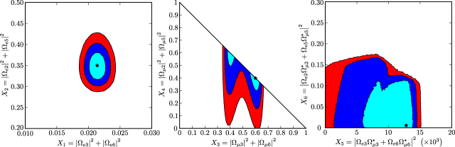
Figure 9: One, two and three $\sigma$ regions in the $\left(X_{1},X_{2}\right)$, $\left(X_{3},X_{4}\right)$ and $\left(X_{5},X_{6}\right)$ which are allowed by electron neutrino survival data from at KamLAND, DayaBay, SuperK and Borexino, muon neutrino survival data at MINOS and T2K and muon to electron transition data from T2K. This plots were obtained from a 7-dimensional scan of the $X_{i}$ defined in eqs. (67)–(70) and marginalizing over 5 variables.

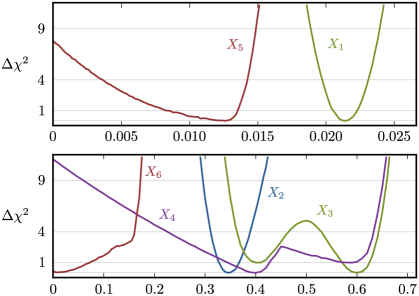
Figure 10: Marginalized $\Delta\chi^{2}$ values for the variables $X_{1,\cdots,6}$ defined in eqs. (67)–(70). The $\chi^{2}$ function for $X_{7}$ is essentially flat. These parameters are a function of the entries of the mixing matrix only; no mass splittings $\varepsilon_{i}$ were considered.

Overall, the bounds on these 7 parameters are broadly consistent with the standard three neutrino oscillation picture. In other words, by substituting in expressions (75)–(78) the numbers obtained for $\theta_{12}$, $\theta_{13}$, $\theta_{23}$ and $\delta$ from global fits [4], we get values for the $X_{i}$ roughly in agreement with figs. (9) and (10). In order to see clearly that current data is consistent with the Dirac limit, note that in this latter case there are only 4 independent parameters. Thus, it follows that the standard three neutrino oscillation picture must correspond to three relations among the 7 $X_{i}$. These are

$$X_{5}=X_{1}X_{3}\,,\,X_{6}=X_{2}X_{4}\textrm{ and }\textrm{Re}\left(X_{7}\right)=\frac{1}{2}\left(1-X_{1}-X_{2}-X_{3}-X_{4}+X_{1}X_{4}+X_{2}X_{3}\right)\,,$$ (79)

and from fig. (11) one can see that oscillation data is compatible with each of these equalities within $\sim 1\sigma$. The three together are disfavored only at $\min\left(\chi_{\textrm{Dirac}}^{2}\right)-\min\left(\chi^{2}\right)=1.9$ so, assuming no mass splittings $\varepsilon_{i}$, there is currently no significant indication for quasi-Dirac neutrinos.

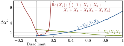
Figure 11: $\Delta\chi^{2}$ functions for the three combinations of parameters which, when equal to 0 simultaneously, signal the Dirac limit (see eq. (79)).

We would like to point out that even in the absence of new mass scales, quasi-Dirac neutrinos can, in principle, be distinguished from some other scenarios through oscillation experiments. In particular, consider 3 active neutrinos and a non-unitary $3\times 3$ mixing matrix $V$. The oscillation probabilities are then given by the expressions

$$P\left(\nu_{e}\rightarrow\nu_{e}\right) =F\left(J_{ee}^{12},J_{ee}^{13},J_{ee}^{23}\right)+J_{ee}^{12}\mathcal{A}_{12}+J_{ee}^{13}\mathcal{A}_{13}+J_{ee}^{23}\mathcal{A}_{23}\,,$$ (80)

$$P\left(\nu_{\mu}\rightarrow\nu_{\mu}\right) =F\left(J_{\mu\mu}^{12},J_{\mu\mu}^{13},J_{\mu\mu}^{23}\right)+J_{\mu\mu}^{12}\mathcal{A}_{12}+J_{\mu\mu}^{13}\mathcal{A}_{13}+J_{\mu\mu}^{23}\mathcal{A}_{23}\,,$$ (81)

$$P\left(\nu_{e}\rightarrow\nu_{\mu}\right) =F^{\prime}\left(J_{ee}^{12},J_{ee}^{13},J_{ee}^{23},J_{\mu\mu}^{12},J_{\mu\mu}^{13},J_{\mu\mu}^{23},J_{e\mu}^{12},J_{e\mu}^{13},J_{e\mu}^{23}\right)+\textrm{Re}\left(J_{e\mu}^{12}\right)\mathcal{A}_{12}+\textrm{Re}\left(J_{e\mu}^{13}\right)\mathcal{A}_{13}$$

$$+\textrm{Re}\left(J_{e\mu}^{23}\right)\mathcal{A}_{23}+\textrm{Im}\left(J_{e\mu}^{12}\right)\mathcal{B}_{12}+\textrm{Im}\left(J_{e\mu}^{13}\right)\mathcal{B}_{13}+\textrm{Im}\left(J_{e\mu}^{23}\right)\mathcal{B}_{23}\,,$$ (82)

where $J_{\alpha\beta}^{ij}=V_{\alpha i}^{*}V_{\beta j}^{*}V_{\beta i}V_{\alpha j}$. The exact form of the functions $F$ and $F^{\prime}$ which control the 0-distance neutrino behavior is not important for the present discussion. The more important point is that with a non-unitary $V$ one can have an oscillatory behavior which is impossible to reproduce with quasi-Dirac neutrinos, and vice-versa.

For example, the $\mathcal{B}_{ij}$ coefficients in $P\left(\nu_{e}\rightarrow\nu_{\mu}\right)$ do not need to be related for a non-unitary $V$, while for quasi-Dirac neutrinos they must be the same (up to a minus sign — see eq. (66)). On the other hand, note that from the $J_{ee}^{ij}$ and $J_{\mu\mu}^{ij}$ one can extract the modulus of the absolute value of all $J_{e\mu}^{ij}$, hence by measuring $P\left(\nu_{e}\rightarrow\nu_{e}\right)$ and $P\left(\nu_{\mu}\rightarrow\nu_{\mu}\right)$, as well as the coefficients $\mathcal{B}_{ij}$ in $P\left(\nu_{e}\rightarrow\nu_{\mu}\right)$, the coefficients of the oscillatory factors $\mathcal{A}_{ij}$ in $P\left(\nu_{e}\rightarrow\nu_{\mu}\right)$ are fixed for a non-unitary $V$ (up to $\pm$ signs). However, for quasi-Dirac neutrinos no such constraint exists. So, with this short theoretical argument, one can conclude that in principle these two non-standard neutrino scenarios can be distinguished through oscillation experiments.

4 Summary

In general, neutrinos can have lepton number violating (Majorana) and lepton number conserving (Dirac) mass terms. If the lepton number violating mass terms are smaller than the lepton number preserving ones, neutrinos are quasi-Dirac particles. Phenomenologically, this corresponds to the existence of three pairs of neutrinos with slightly different masses, hence oscillation experiments are sensitive not only to the usual solar and atmospheric mass scales, but also to three small mass splittings $\varepsilon_{i}$. Furthermore, for quasi-Dirac neutrinos there are more than 3+1 angles and phases to be considered. In this work, we have analyzed the constraints on these quasi-Dirac neutrino parameters imposed by current neutrino oscillation data and also briefly discussed the potential of the future JUNO experiment to improve upon existing constraints.

In section (2) we have discussed a fully general parametrization of the lepton sector for three generations of quasi-Dirac neutrinos. In addition to the charged lepton masses, there is a total of 6 masses, 12 angles and 12 phases. Oscillation experiments are not sensitive to the overall neutrino mass scale nor to 5 of the phases (which are of the Majorana type). Hence we are left with a 24-dimensional model space, compared to the six-dimensional space for an ordinary three generation case ($\Delta m^{2}_{\odot}$, $\Delta m^{2}_{\rm Atm}$, $\theta_{12}$, $\theta_{13}$, $\theta_{23}$ and $\delta$).

It is numerically too costly to handle such a large number of parameters at the same time, hence we analyzed several different special cases. First, we took a single mass splitting $\varepsilon_{i}^{2}\neq 0$. If we split two neutrinos with mass $m_{i}$ into a quasi-degenerate pair of particles with masses $\sqrt{m_{i}^{2}-\varepsilon_{i}^{2}/2}$ and $\sqrt{m_{i}^{2}+\varepsilon_{i}^{2}/2}$ then a new oscillation length $L\propto 1/\varepsilon_{i}^{2}$ appears which is associated to the conversion of active to sterile neutrinos. Very stringent limits on $\varepsilon_{i}^{2}$ in such one parameter extensions can be derived, of the order of $10^{-11}\textrm{ eV}^{2}$ for $\varepsilon_{1,2}^{2}$ (from solar neutrino data) and $10^{-5}\textrm{ eV}^{2}$ for $\varepsilon_{3}^{2}$ (dominated by Super-K atmospheric neutrino data).

Next, we considered the case when one mass splitting and one of the non-standard angles are allowed to take non-zero values at the same time. As we have shown, in this situation degeneracies of the $\chi^{2}$ function can occur, implying that from a single experiment in many cases it will no longer be possible to derive meaningful limits on individual parameters. These degeneracies can be resolved by considering data from more than one experiment, accessing different $P\left(\nu_{\alpha}\rightarrow\nu_{\beta}\right)$.

We then considered the possibility of nullifying the effects of the $\varepsilon_{i}$ completely by changing some particular combinations of the angles $\theta_{ij}$ of our parametrization. Instead of pursuing the exact form of these rather complex parameter combinations, we discussed a simpler definition, describing 3 angles $\varphi_{i}$ associated to rotations between the columns $i$ and $i+3$ of the quasi-Dirac mixing matrix, such that in the limit where these angles are equal to $\pi/4$ ($3\pi/4$) the $i+3$($i$) column of the mixing matrix vanishes and hence the associated neutrino mass disappears from the oscillation probability formula. We stress that for these particular parameter combinations no limits on the $\varepsilon_{i}$ can be derived from oscillation experiments. The regions in the planes $(\varepsilon_{i},\varphi_{i})$ which are allowed by various experiments are shown in figs. (5) and (7). In this context, it is interesting to note that the tension between the value of the solar mass scale preferred by global fits ($\sim 7.6\times 10^{-3}\textrm{ eV}^{2}$) and the lower one preferred by solar data ($\sim 4\times 10^{-3}\textrm{ eV}^{2}$) might be resolved by a non-zero value for either $\varepsilon_{1}$ or $\varepsilon_{2}$.

Lastly, we considered the possibility that the mass splittings $\varepsilon_{i}$ are too small to be measured in oscillation experiments. Even in this scenario, one can have departures from the lepton-number-conserving Dirac scenario due to the new angles $\theta_{ij}$ (and phases $\phi_{ij}$). As mentioned above, there is a large number of such parameters. However, it can be shown that with 3 pairs of neutrinos with the same mass, oscillations will only depend on a total of 13 combinations of angles and phases. Additionally, if we focus just on electron and muon neutrinos, this number is further reduced to 7, corresponding to 6 angles and 1 phase. In the text we called these parameter combinations $X_{1\cdots 7}$ and stressed that they can not be identified with $\theta_{12}$, $\theta_{13}$, $\theta_{23}$ nor $\delta$, as these quantities by themselves are not physical. Instead, the 7 $X_{i}$ correspond to combinations of these and additional $\theta_{ij}$ angles and $\phi_{ij}$ phases.

In section (3.2) we made a 7-dimensional scan of these $X_{i}$ parameters in the absence of mass splittings. Their exact definitions, as well as the limits imposed on them by current data can be found there. Crucially, for Dirac neutrinos there are only 4 parameters. Hence the Dirac limit corresponds to 3 relations among the 7 $X_{i}$. By testing these relations, we find that $\min\left(\chi_{\textrm{Dirac}}^{2}\right)-\min\left(\chi^{2}\right)=1.9$, i.e. current data is compatible with the Dirac scenario. Progress on tests for quasi-Diracness can be made in the future with a more precise measurement of $P\left(\nu_{e}\rightarrow\nu_{\mu}\right)$ and $P\left(\nu_{\mu}\rightarrow\nu_{\mu}\right)$. Thus, more statistics taken in T2K, MINOS+ or NO$\nu$A and, in particular, the future precise measurements possible at DUNE should provide more sensitive probes for this particular setup of quasi-Dirac neutrinos without new mass scales.

References

- [1] I. Avignone, Frank T., S. R. Elliott and J. Engel, Double beta decay, Majorana neutrinos, and neutrino mass, Rev.Mod.Phys. 80 (2008) 481–516, arXiv:0708.1033 [nucl-ex].
- [2] F. F. Deppisch, M. Hirsch and H. Päs, Neutrinoless double-beta decay and physics beyond the Standard Model, J.Phys. G39 (2012) 124007, arXiv:1208.0727 [hep-ph].
- [3] S. Abe et al. (KamLAND), Precision measurement of neutrino oscillation parameters with KamLAND, Phys. Rev. Lett. 100 (2008) 221803, arXiv:0801.4589 [hep-ex].
- [4] P. F. de Salas et al., Status of neutrino oscillations 2017 (2017), arXiv:1708.01186 [hep-ph].
- [5] L. Wolfenstein, Different varieties of massive Dirac neutrinos, Nucl. Phys. B186 (1981) 147–152.
- [6] J. W. F. Valle, Neutrinoless double- decay with quasi-Dirac neutrinos, Phys. Rev. D27 (1983) 1672–1674.
- [7] S. T. Petcov, On pseudo-Dirac neutrinos, neutrino oscillations and neutrinoless double -decay, Phys. Lett. 110B (1982) 245–249.
- [8] M. Doi et al., Pseudo Dirac neutrino, Prog. Theor. Phys. 70 (1983) 1331.
- [9] G. Dutta and A. S. Joshipura, Pseudo Dirac neutrinos in the seesaw model, Phys. Rev. D51 (1995) 3838–3842, arXiv:hep-ph/9405291 [hep-ph].
- [10] A. S. Joshipura and S. D. Rindani, Phenomenology of pseudo Dirac neutrinos, Phys. Lett. B494 (2000) 114–123, arXiv:hep-ph/0007334 [hep-ph].
- [11] S. M. Bilenky and B. Pontecorvo, Neutrino oscillations with large oscillation length in spite of large (Majorana) neutrino masses?, Sov. J. Nucl. Phys. 38 (1983) 248, [Yad. Fiz.38,415(1983)].
- [12] S. M. Bilenky and S. T. Petcov, Massive neutrinos and neutrino oscillations, Rev. Mod. Phys. 59 (1987) 671, [Erratum: Rev. Mod. Phys.60,575(1988)].
- [13] C. Giunti, C. W. Kim and U. W. Lee, Oscillations of pseudo Dirac neutrinos and the solar-neutrino problem, Phys. Rev. D46 (1992) 3034–3039, arXiv:hep-ph/9205214 [hep-ph].
- [14] Y. Nir, Pseudo-Dirac solar neutrinos, JHEP 06 (2000) 039, arXiv:hep-ph/0002168 [hep-ph].
- [15] P. H. Frampton, M. C. Oh and T. Yoshikawa, Zee model confronts SNO data, Phys. Rev. D65 (2002) 073014, arXiv:hep-ph/0110300 [hep-ph].
- [16] X.-G. He, Is the Zee model neutrino mass matrix ruled out?, Eur. Phys. J. C34 (2004) 371–376, arXiv:hep-ph/0307172 [hep-ph].
- [17] B. Brahmachari and S. Choubey, Viability of bimaximal solution of the Zee mass matrix, Phys. Lett. B531 (2002) 99–104, arXiv:hep-ph/0111133 [hep-ph].
- [18] A. Zee, A theory of lepton number violation and neutrino Majorana masses, Phys.Lett. B93 (1980) 389. [Erratum: Phys. Lett.95B,461(1980)].
- [19] A. Geiser, Pseudo-Dirac neutrinos as a potential complete solution to the neutrino oscillation puzzle, Phys. Lett. B444 (1999) 358, arXiv:hep-ph/9901433 [hep-ph].
- [20] W. Krolikowski, Option of three pseudo-Dirac neutrinos, Acta Phys. Polon. B31 (2000) 663–672, arXiv:hep-ph/9910308 [hep-ph].
- [21] K. R. S. Balaji, A. Kalliomaki and J. Maalampi, Revisiting pseudo-Dirac neutrinos, Phys. Lett. B524 (2002) 153–160, arXiv:hep-ph/0110314 [hep-ph].
- [22] E. Ma and P. Roy, Model of four light neutrinos in the light of all present data, Phys. Rev. D52 (1995) R4780–R4783, arXiv:hep-ph/9504342 [hep-ph].
- [23] S. Goswami and A. S. Joshipura, Neutrino anomalies and quasi Dirac neutrinos, Phys. Rev. D65 (2002) 073025, arXiv:hep-ph/0110272 [hep-ph].
- [24] A. de Gouvea, W.-C. Huang and J. Jenkins, Pseudo-Dirac neutrinos in the new Standard Model, Phys. Rev. D80 (2009) 073007, arXiv:0906.1611 [hep-ph].
- [25] M. Cirelli, G. Marandella, A. Strumia and F. Vissani, Probing oscillations into sterile neutrinos with cosmology, astrophysics and experiments, Nucl. Phys. B708 (2005) 215–267, arXiv:hep-ph/0403158 [hep-ph].
- [26] J. F. Beacom et al., Pseudo-Dirac neutrinos: A challenge for neutrino telescopes, Phys. Rev. Lett. 92 (2004) 011101, arXiv:hep-ph/0307151 [hep-ph].
- [27] A. Esmaili, Pseudo-Dirac neutrino scenario: Cosmic neutrinos at neutrino telescopes, Phys. Rev. D81 (2010) 013006, arXiv:0909.5410 [hep-ph].
- [28] A. Esmaili and Y. Farzan, Implications of the pseudo-Dirac scenario for ultra high energy neutrinos from GRBs, JCAP 1212 (2012) 014, arXiv:1208.6012 [hep-ph].
- [29] A. S. Joshipura, S. Mohanty and S. Pakvasa, Pseudo-Dirac neutrinos via a mirror world and depletion of ultrahigh energy neutrinos, Phys. Rev. D89 (2014) 3 033003, arXiv:1307.5712 [hep-ph].
- [30] M. Kobayashi and C. S. Lim, Pseudo Dirac scenario for neutrino oscillations, Phys. Rev. D64 (2001) 013003, arXiv:hep-ph/0012266 [hep-ph].
- [31] Y. H. Ahn, S. K. Kang and C. S. Kim, A model for pseudo-Dirac neutrinos: leptogenesis and ultra-high energy neutrinos, JHEP 10 (2016) 092, arXiv:1602.05276 [hep-ph].
- [32] G. J. Stephenson, Jr., J. T. Goldman, B. H. J. McKellar and M. Garbutt, Large mixing from small: Pseudo-Dirac neutrinos and the singular see-saw, Int. J. Mod. Phys. A20 (2005) 6373–6390, arXiv:hep-ph/0404015 [hep-ph].
- [33] K. L. McDonald and B. H. J. McKellar, The type-II singular see-saw mechanism, Int. J. Mod. Phys. A22 (2007) 2211–2222, arXiv:hep-ph/0401073 [hep-ph].
- [34] R. Mohapatra and J. Valle, Neutrino mass and baryon-number nonconservation in superstring models, Phys. Rev. D34 (1986) 1642.
- [35] D. Chang and O. C. W. Kong, Pseudo-Dirac neutrinos, Phys. Lett. B477 (2000) 416–423, arXiv:hep-ph/9912268 [hep-ph].
- [36] V. Berezinsky, M. Narayan and F. Vissani, Mirror model for sterile neutrinos, Nucl. Phys. B658 (2003) 254–280, arXiv:hep-ph/0210204 [hep-ph].
- [37] L. A. Sanchez, W. A. Ponce and R. Martinez, as an subgroup, Phys. Rev. D64 (2001) 075013, arXiv:hep-ph/0103244 [hep-ph].
- [38] R. M. Fonseca and M. Hirsch, Lepton number violation in 331 models, Phys. Rev. D94 (2016) 11 115003, arXiv:1607.06328 [hep-ph].
- [39] S. Abel, A. Dedes and K. Tamvakis, Naturally small Dirac neutrino masses in supergravity, Phys. Rev. D71 (2005) 033003, arXiv:hep-ph/0402287 [hep-ph].
- [40] Q. R. Ahmad et al. (SNO), Direct evidence for neutrino flavor transformation from neutral-current interactions in the Sudbury Neutrino Observatory, Phys. Rev. Lett. 89 (2002) 011301, arXiv:nucl-ex/0204008 [nucl-ex].
- [41] K. Abe et al. (Super-Kamiokande), Limits on sterile neutrino mixing using atmospheric neutrinos in Super-Kamiokande, Phys. Rev. D91 (2015) 052019, arXiv:1410.2008 [hep-ex].
- [42] N. Agafonova et al. (OPERA), Limits on muon-neutrino to tau-neutrino oscillations induced by a sterile neutrino state obtained by OPERA at the CNGS beam, JHEP 06 (2015) 069, arXiv:1503.01876 [hep-ex].
- [43] P. Adamson et al. (MINOS, Daya Bay), Limits on active to sterile neutrino oscillations from disappearance searches in the MINOS, Daya Bay, and Bugey-3 experiments, Phys. Rev. Lett. 117 (2016) 15 151801, [Publisher’s Note: Phys. Rev. Lett. 117, 209901], arXiv:1607.01177 [hep-ex].
- [44] M. G. Aartsen et al. (IceCube), Search for sterile neutrino mixing using three years of IceCube DeepCore data, Phys. Rev. D95 (2017) 11 112002, arXiv:1702.05160 [hep-ex].
- [45] P. Adamson et al. (NOvA), Search for active-sterile neutrino mixing using neutral-current interactions in NOvA (2017), arXiv:1706.04592 [hep-ex].
- [46] K. N. Abazajian et al., Light sterile neutrinos: A white paper (2012), arXiv:1204.5379 [hep-ph].
- [47] S. Gariazzo et al., Light sterile neutrinos, J. Phys. G43 (2016) 033001, arXiv:1507.08204 [hep-ph].
- [48] J. Schechter and J. W. F. Valle, Neutrino masses in theories, Phys. Rev. D22 (1980) 2227.
- [49] K. Abe et al. (Super-Kamiokande), Solar neutrino measurements in Super-Kamiokande-IV, Phys. Rev. D94 (2016) 5 052010, arXiv:1606.07538 [hep-ex].
- [50] G. Bellini et al. (BOREXINO), Neutrinos from the primary proton-proton fusion process in the Sun, Nature 512 (2014) 7515 383–386.
- [51] G. Bellini et al., Precision measurement of the solar neutrino interaction rate in Borexino, Phys. Rev. Lett. 107 (2011) 141302, arXiv:1104.1816 [hep-ex].
- [52] T. Kajita, The measurement of neutrino properties with atmospheric neutrinos, Ann. Rev. Nucl. Part. Sci. 64 (2014) 343–362.
- [53] P. Adamson et al. (MINOS), Measurement of neutrino and antineutrino oscillations using beam and atmospheric data in MINOS, Phys. Rev. Lett. 110 (2013) 25 251801, arXiv:1304.6335 [hep-ex].
- [54] K. Abe et al. (T2K), Measurements of neutrino oscillation in appearance and disappearance channels by the T2K experiment with protons on target, Phys. Rev. D91 (2015) 7 072010, arXiv:1502.01550 [hep-ex].
- [55] F. P. An et al. (Daya Bay), Measurement of electron antineutrino oscillation based on 1230 days of operation of the Daya Bay experiment, Phys. Rev. D95 (2017) 7 072006, arXiv:1610.04802 [hep-ex].
- [56] F. An et al. (JUNO), Neutrino physics with JUNO, J. Phys. G43 (2016) 3 030401, arXiv:1507.05613 [physics.ins-det].