Comparison of the linear bias models in the light of the Dark Energy Survey

Abstract

The evolution of the linear and scale independent bias, based on the most popular dark matter bias models within the $\Lambda$CDM cosmology, is confronted to that of the Dark Energy Survey (DES) Luminous Red Galaxies (LRGs). Applying a $\chi^{2}$ minimization procedure between models and data we find that all the considered linear bias models reproduce well the LRG bias data. The differences among the bias models are absorbed in the predicted mass of the dark-matter halo in which LRGs live and which ranges between $\sim 6\times 10^{12}h^{-1}M_{\odot}$ and $1.4\times 10^{13}h^{-1}M_{\odot}$, for the different bias models. Similar results, reaching however a maximum value of $\sim 2\times 10^{13}h^{-1}M_{\odot}$, are found by confronting the SDSS (2SLAQ) Large Red Galaxies clustering with theoretical clustering models, which also include the evolution of bias. This later analysis also provides a value of $\Omega_{m}=0.30\pm 0.01$, which is in excellent agreement with recent joint analyses of different cosmological probes and the reanalysis of the Planck data.

Keywords: cosmology: dark matter halo, bias

1 Introduction

Studies of the distribution of matter on large-scales, based on different mass tracers (galaxies, clusters etc), can be used to test the validity of different models of structure formation. However, an important issue that significantly affects such an approach is our limited knowledge of how luminous matter traces the background mass density field. The so-called biasing between different extragalactic sources and the underlying matter distribution was first introduced (e.g. Kaiser 1984, Bardeen et. al. 1986) in order to explain the lower amplitude of the 2-point correlation function of galaxies with respect to that of galaxy clusters.

The most common biasing models consider the Large Scale Structures (LSS) as high peaks of an initially random Gaussian density field, while assuming scale-independence (mostly above $5h^{-1}$ Mpc) and linearity. Following the above lines the linear bias parameter is defined as the ratio of the fluctuations of the mass tracer ($\delta_{tr}$) to that of the underlying mass ($\delta_{m}$):

$$b=\frac{\delta_{tr}}{\delta_{m}}\;.$$ (1)

Due to the fact that the two point correlation function is written as $\xi(r)=\langle\delta(x)\delta(x+r)\rangle$, one can easily show that the bias factor is also given by:

$$b=\left(\frac{\xi_{tr}}{\xi_{m}}\right)^{1/2}$$ (2)

or

$$b=\left(\frac{\sigma_{8,tr}}{\sigma_{8,m}}\right)^{1/2}$$ (3)

where $\sigma^{2}_{8,i}=\xi_{i}(0)=\langle\delta^{2}_{i}(x)\rangle$ is the mass variance at $R_{8}=8h^{-1}$ Mpc ($i$ corresponding to $tr$ or $m$).

In the literature there is a large body of scenarios that attempt to predict the cosmological evolution of the bias parameter and in general, there are two main categories of analytic bias evolution models (for more details see Papageorgiou et. al. 2012 and the references therein). The first family of models corresponds to the so-called galaxy merging bias which is based on the Press-Schechter formalism (1974), the peak background split [Bardeen et al. 1986] and the spherical collapse model (Cole & Kaiser 1989; Mo & White 1996; Matarrese et. al. 1997; Moscardini et. al. 1998; Sheth & Tormen 1999; Valageas 2009, 2011). The difference between the predictions of these bias models with respect to those of numerical simulations have led the authors to introduce modifications to the models by using ellipsoidal collapse [Sheth, Mo & Tormen 2001], new fitting bias formulas (Jing 1998; Tinker et. al. 2005) and a non-Markovian extension of the excursion set theory (Ma et. al. 2011; de Simone et. al. 2011).

The second family assumes a continuous mass-tracer fluctuation field, which is proportional to that of the underlying mass. In this framework, the mass tracers act as “test particles”. This family can be divided into two sub-groups:

• The first one is the galaxy conserving bias model. This model utilizes the continuity equation and the assumption that the extragalactic tracers and underlying mass share the same velocity field (Nusser & Davis 1994; Fry 1996; Tegmark & Peebles 1998; Hui & Parfrey 2008; Schaefer, Douspis & Aghanim 2009). In this context, the evolution of bias is given by $b(z)=1+(b_{0}-1)/D(z)$, as the solution of a 1st order differential equation. Notice, that $D(z)$ is the growth factor of density perturbations (scaled to unity at the present time) and $b_{0}$ is the bias factor at the present epoch. It is well known that this bias model has two fundamental problems. The first one is related with the anti-biased problem, the fact that an anti-biased set of tracers at the present time ($b_{0}<1$) remains always anti-biased at high redshifts. The second problem is based on the fact that this model shows a realistic bias evolution only at low redshifts $z\leq 0.5$ [Bagla 1998].

• This subfamily is basically an extension of the previous one but free of the above problematic issues. Specifically, it utilizes the three hydrodynamical equations of motion (continuity, Euler and Poisson equations) in the linear regime and the fact that the underlying mass and extragalactic mass-tracers feel the same gravity field, but they do not not necessarily share the same velocity field. The combination of the above ingredients provide a second order differential equation in $b$, the solution of which gives the evolution of the linear bias factor (Basilakos & Plionis 2001, 2003; Basilakos, Plionis & Ragone-Figueroa 2008; Basilakos, Plionis & Pouri 2011). It is interesting to mention that this bias formula is valid for all dark energy models including those of modified gravity (see Basilakos, Plionis & Pouri 2011; Basilakos et. al. 2012).

It should be mentioned that the linear bias model relates a mass tracer, being a galaxy, an Active Galactic Nuclei (AGN), a Luminous Red Galaxy (LRG) or a cluster of galaxies, with a host dark matter halo within which the mass tracer forms and evolves. The models themselves follow the linear evolution of the host halo and not the internal evolution of the astrophysical processes of the tracer. Thus the assumption is that the effects of nonlinear gravity and hydrodynamics (merging, feedback mechanisms, etc.) can be ignored in the linear-regime (Catelan et al. 1998) and that each DM halo hosts only one mass tracer.

Recently, the deterministic and linear nature of bias has been challenged (see McDonald et. al. 2009; Chan et al. 2012), and indeed a large body of papers have been published studying the evolution of bias in the non-linear and non-local regimes respectively (Paranjape et. al. 2013; Assasi et. al. 2014; Di Porto et. al. 2016; Lazeyras et. al. 2016; Desjacques et. al. 2016 and references therein). Morever, numerical simulations have been used in several studies (Hoffmann et. al. 2017, Hoffmann et. al. 2015, Baldauf et. al. 2012; Bel et. al. 2015) towards investigating the nature of bias and they found deviations from the linear regime. Despite the above considerations, the linear biasing assumption has a long history in cosmology and it is still a useful first-order approximation which, because of its simplicity, is used in studies of large-scale (linear) dynamics. For example, the Dark Energy Survey (DES) team (Elvin-Poole et al. 2017) used the clustering properties of the Luminous Red Galaxies (LRGs) in order to measure the evolution of bias in the linear regime.

In the present paper we investigate the predictions of the most popular of the above linear bias models. Utilizing the linear bias data of Luminous Red Galaxies (LRGs), recently released by the DES group but also of the SDSS DR5 data, we test the range of validity of the explored bias models. In particular, the outline of this paper is as follows. In Section 2 we provide the LRGs bias data based on the 1-year DES sample. In Section 3 we introduce the main elements of the bias evolution models. In Section 4 we present the outcome of the current analysis, while in Section 5 we compare the DES results with those of SDSS DR5 LRGs data, using the 2 point angular correlation function data. In Section 6 we provide our conclusions.

Finally, we would like to spell out clearly which are the basic assumptions of our work, which are common to many studies of the bias: (a) the biasing is linear on the scales of interest (which does not preclude being scale dependent on small non-linear scales), and (b) each dark matter halo is populated by one extragalactic mass tracer (in our case LRG).

2 DESY1 Red Galaxies Bias Data

The application of the correlation function analysis on samples of high redshift extragalactic sources for cosmological studies has a long history (cf. Basilakos 2001; Matsubara 2004). For example, in a sequence of previous publications some of us used the clustering properties of the XMM-Newton X-ray sources in order to place constraints on the dark energy models (Basilakos & Plionis, 2005, 2006, 2009, 2010).

In the current work we will use as tracers of the LSS the Luminous Red Galaxies (LRGs), which according to Eisenstein et. al. (2001), and due to their high luminosities, are very useful tracers of the LSS. One important advantage is that such a population can be observed up to relatively large redshifts. In particular, we will use the DES bias data provided by Elvin-Poole et al. (2017). These bias data were extracted with the aid of the angular correlation function (ACF), which was estimated in Elvin-Poole et. al. (2017), using the 1-year DES sample of $\sim 6.6\times 10^{5}$ LRGs in the redshift range $0.15<z<0.9$.

These authors used the assumption of linear bias in the derivation of the DES bias data. According to Krause et. al. (2017) the scale of $\sim 8h^{-1}$Mpc, used by the DES team, ensures that the impact of non-linear effects on clustering and thus on biasing is almost negligible. Moreover, in order to measure the DES bias the above authors have fixed the cosmological parameters at the mean of the so called DESY1COSMO posterior, namely $\Omega_{m}=1-\Omega_{\Lambda}=0.276$, $h=0.7619$, $\Omega_{b}=0.0526$ and spectral index $n=0.9964$.

Although we will utilize the bias data provided by the previous references, for completion we rescale the bias data using different references cosmologies. Specifically, we wish to convert the value of bias data from the DESY1COSMO cosmological model, say DES, to another, say A. Utilizing the definition of bias and the notations of Papageorgiou et. al. (2012) the scaling relation from the DESY1COSMO model to that of A, takes the form:

$$b_{A}(z)\simeq b_{B}(z)\frac{\sigma_{8,B}}{\sigma_{8,A}}\frac{D_{B}(z)}{D_{A}(z)}\\$$ (4)

where the index $B$ corresponds to DES, $\sigma_{8}$ is the present value of the mass variance at $8h^{-1}Mpc$ and $D(z)$ is the growth factor of matter fluctuations in the linear regime. Also, the normalized Hubble parameter of the $\Lambda$CDM model is given by

$$E(z)=\left[\Omega_{m}(1+z)^{3}+\Omega_{\Lambda}\right]^{1/2}\;.$$ (5)

where $\Omega_{\Lambda}=1-\Omega_{m}$.

In the current article we convert the bias data to the following basic $\Lambda$CDM cosmologies:

• Planck TT+lowP+lensing results, namely $\Omega_{m}=1-\Omega_{\Lambda}=0.308$, $h=0.678$, $n=0.9671$, $\Omega_{b}=0.0484$ and $\sigma_{8}=0.815$. The latter cosmological parameters are in agreement with those of the reanalysis of the Planck data provided by Spergel et al. (2015).

• Finally, we utilize the DES/Planck/JLA/BAO joint likelihood results, namely $\Omega_{m}=1-\Omega_{\Lambda}=0.301$, $h=0.682$, $\Omega_{b}=0.048$, $n=0.973$ and $\sigma_{8}=0.801$ (see Abbott et al. 2017).

In Table 1 we present the precise numerical values of the DES bias data with the corresponding errors that are used in our analysis. Also, in the last two columns of Table 1 we provide with the aid of Eq.(4) the Planck-scaled and DES/Planck/JLA/BAO-scaled bias data respectively.

Red. Range	Median Redshift	DESY1 bias	Planck-scaled bias	DES/Planck/JLA/BAO-scaled bias
$0.15<z<0.3$	$0.225\pm 0.075$	$1.40\pm 0.077$	$1.434\pm 0.079$	$1.457\pm 0.080$
$0.3<z<0.45$	$0.375\pm 0.075$	$1.61\pm 0.051$	$1.655\pm 0.052$	$1.680\pm 0.053$
$0.45<z<0.6$	$0.525\pm 0.075$	$1.60\pm 0.040$	$1.649\pm 0.041$	$1.673\pm 0.042$
$0.6<z<0.75$	$0.675\pm 0.075$	$1.93\pm 0.045$	$1.994\pm 0.047$	$2.022\pm 0.047$
$0.75<z<0.9$	$0.825\pm 0.075$	$1.99\pm 0.066$	$2.060\pm 0.068$	$2.088\pm 0.069$

Table 1: The measured bias data of the 1-year DES LRGs from Elvin-Poole et. al. (2017).

3 Bias Models

In this section we briefly present the most popular bias models. Specifically, from the galaxy merging bias family we will investigate the models of Sheth, Mo & Tormen (2001) [hereafter SMT], the Jing (1998) the Tinker et. al. (2010) [hereafter TRK], de Simone et. al. (2011) [hereafter DMR] and the Ma et. al. (2011) [hereafter MMRZ]. In this case the bias factor is given as a function of the peak-height parameter, $\nu=\delta_{c}(z)/\sigma(M_{h},z)$ where $\delta_{c}$ is the linearly extrapolated density threshold above which structures collapse. In the present study we utilize the accurate fitting formula of Weinberg & Kamionkowski (2003) to estimate $\delta_{c}(z)$. Furthermore, the mass variance is written as

$$\sigma(M_{h},z)=\left[\frac{D^{2}(z)}{2\pi^{2}}\int_{0}^{\infty}k^{2}P(k)W^{2}(kR)dk\right]^{1/2}$$ (6)

where $W(kR)=3[sin(kR)-kRcos(kR)]/(kR)^{3}$ is the Fourier transform of the top-hat smoothing kernel with $R=[3M_{h}/(4\pi\rho_{m})]^{1/3}$, $M_{h}$ is the mass of the halo and $\rho_{m}$ is the mean matter density of the universe at the present time. The quantity $P(k,z)$ is the CDM linear power spectrum given by $P(k,z)=P_{0}k^{n}T^{2}(k)D^{2}(z)$ where $n$ is the spectral index of the primordial power spectrum and $T(k)$ is the CDM transfer function provided by Eisenstein & Hu (1998):

$$T(k)=\frac{L_{0}}{L_{0}+C_{0}q^{2}}$$ (7)

with $L_{0}={\rm ln}(2e+1.8q)$, $e=2.718$, $C_{0}=14.2+\frac{731}{1+62.5q}$ and $q=k/\Gamma$ with $\Gamma$ being is the shape parameter given by (Sugiyama 1995):

$$\Gamma=\Omega_{m}h{\rm exp}(-\Omega_{b}-\sqrt{2h}\frac{\Omega_{b}}{\Omega_{m}}).$$

Taking the aforementioned quantities into account and using Eq.(6) the normalization of the power spectrum becomes

$$P_{0}=2\pi^{2}\sigma_{8}^{2}\left[\int_{0}^{\infty}T^{2}(k)k^{n+2}W^{2}(kR_{8})dk\right]^{-1}$$ (8)

where $\sigma_{8}\equiv\sigma(R_{8},0)$.

From the second bias group we will use the generalized model of Basilakos, Plionis & Pouri 2011 (hereafter BPR; see also Basilakos et. al. 2012) which is valid for any dark energy model including those of modified gravity.

Let us now briefly present the functional forms of the aforementioned linear bias models (for more details see Papageorgiou et al. 2012 and references therein), whose dark matter halo masses can be constrained by using the DES bias data:

SMT:

$$b(\nu)=1+\frac{1}{\sqrt{\alpha}}\delta_{c}(z)[\sqrt{\alpha}(\alpha\nu^{2})+\sqrt{\alpha}b(\alpha\nu^{2})^{1-c}-f(\nu)]$$ (9)

with

$$f(\nu)=\frac{(\alpha\nu^{2})^{c}}{(\alpha\nu^{2})^{c}+b(1-c)(1-c/2)},$$ (10)

where $\alpha=0.707,b=0.5,c=0.6$.

JING:

$$b(\nu)=\left(\frac{0.5}{\nu^{4}}+1\right)^{0.06-0.02\nu}\left(1+\frac{\nu^{2}-1}{\delta_{c}}\right)$$ (11)

TRK:

$$b(\nu)=1-A\frac{\nu^{\alpha}}{\nu^{\alpha}+\delta_{c}^{\alpha}}+B\nu^{b}+C\nu^{c}\;,$$ (12)

where $A=1+0.24y$exp$[-(4/y)^{4}]$, $B=0.183$, $C=0.019+0.107y+0.19$exp$[-(4/y)^{4}]$, $\alpha=0.44y-0.88$, $b=1.5$ and $c=2.4$. For $y$ we have $y={\rm log}_{10}\Delta$.

DMR:

$$b(\nu)=1+\sqrt{\alpha}\frac{\nu^{2}}{\delta_{c}}\left[1+0.4\left(\frac{1}{\alpha\nu^{2}}\right)^{0.6}\right]\\ -\frac{1}{\sqrt{\alpha}\delta_{c}\left[1+0.067\left(\frac{1}{\alpha\nu^{2}}\right)^{0.6}\right]}\;,$$ (13)

where $\alpha=0.818$.

MMRZ:

$$b(\nu)=1+\frac{\alpha\nu^{2}-1+\frac{\alpha\kappa}{2}\left[2-e^{\alpha\nu^{2}/2}\Gamma(0,\frac{\alpha\nu^{2}}{2})\right]}{\sqrt{\alpha}\delta_{c}[1-\alpha\kappa+\frac{\alpha\kappa}{2}e^{\alpha\nu^{2}/2}\Gamma(0,\frac{\alpha\nu^{2}}{2})]}\;,$$ (14)

where $\alpha=0.818$ and $\kappa=0.23$.

BPR:

$$b(z)=1+\frac{b_{0}-1}{D(z)}+C_{2}\frac{J(z)}{D(z)}$$ (15)

where

$$b_{0}=0.857\left[1+\left(\frac{\Omega_{m}}{0.27}\frac{M_{h}}{10^{14}h^{-1}M_{\odot}}\right)^{0.55}\right]$$ (16)

and

$$C_{2}=1.105\left(\frac{\Omega_{m}}{0.27}\frac{M_{h}}{10^{14}h^{-1}M_{\odot}}\right)^{0.255}$$ (17)

Notice that the factor $\Omega_{m}/0.27$ comes from the fact that the constants $b_{0}$ and $C_{2}$ where originally computed (Basilakos et al. 2012) using $\Lambda$CDM N-body simulations in the context of WMAP7 cosmology, namely $\Omega_{m}=0.27$ and $\sigma_{8}=0.81$. Interestingly, this $\sigma_{8}$ value is consistent with the most recent Planck analysis of Ade et al. (2015).

4 Fitting Models To The Bias Data

In order to test the range of validity of the aforementioned bias models we use a standard $\chi^{2}$-minimization procedure and compare the measured LRG bias data [Elvin-Poole et al. 2017] with the expected theoretical bias models. In our case the $\chi^{2}$ function is defined as follows:

$$\chi^{2}=\displaystyle\sum^{5}_{i=1}\frac{\left[b_{\rm obs}(z_{i})-b_{\rm th}(\textbf{p},z_{i})\right]^{2}}{\sigma_{i}^{2}+\sigma_{z}^{2}}$$ (18)

where ${\bf p}$ is a vector containing the free parameter that we want to constrain. Also, $\sigma_{i}$ is the uncertainties of the observed bias (see Table 1). The fact that the DES bias data are given in redshift intervals implies that we need to introduce an additional uncertainty in the $\chi^{2}$ estimator. In our case we choose this uncertainty to be equal to the width of the redshift bin, $\sigma_{z}=0.075$. It becomes clear that our statistical analysis contains one independent free parameter, hence the statistical vector ${\bf p}$ is associated with the environment of the dark matter halo in which the mass tracers (in our case LRGs galaxies) live, namely ${\bf p}=M_{h}$.

To this end we utilize, the corrected Akaike information criterion which is appropriate for small sample size, (Akaike 1974, Sugiura 1978). Considering Gaussian errors the AIC_c estimator becomes (see Liddle 2007)

$${\rm AIC}_{c}=\chi^{2}_{\rm min}+2k+\frac{2k(k+1)}{N-k-1}$$ (19)

where $N$ is the number of data (5 in our case), $k$ is the number of free parameters, and thus when $k=1$ then AIC${}_{c}=\chi^{2}_{\rm min}+10/3$. A smaller value of AIC points a better model-data fit. Moreover, in order to explore, the effectiveness of the different models in reproducing the observational data, we need to introduce the model pair difference, namely $\Delta$AIC=AIC_c,x-AIC_c,y. Therefore, the higher the value of $|{\rm\Delta AIC}|$, the higher the evidence against the model with higher value of AIC_c, with a difference $4\leq|{\rm\Delta AIC}|\leq 7$ (Burnham & Anderson 2002; Burnham & Anderson 2004) suggesting a positive such evidence and $|{\rm\Delta AIC}|\geq 10$ suggesting a strong such evidence. Notice, that if $|{\rm\Delta AIC}|\leq 2$ then this is a indication of consistency among the two comparison models

Our main statistical results are presented in Table 2, where we quote the fitted halo mass with the corresponding $1\sigma$ uncertainties and the goodness of fit statistics ($\chi^{2}$ and AIC_c), for three different expansion models (see section 2). After considering the best-$\chi^{2}$ and the value of the Akaike information criterion we find that most bias models fit at a statistically acceptable level the DES bias data. The best model is the SMT, while we find a tension between the MMRZ model and the bias data, $|\Delta$AIC$|=|{\rm AIC}_{c,\rm SMT}-{\rm AIC}_{c,\rm MMRZ}|>4$. We observe that the BPR and the TRK bias models predict consistent values (within $1\sigma$) of dark matter halos with that of SMT. Lastly, the fact $|\Delta$AIC$|\leq 2$ implies that the SMT bias model is statistically equivalent with those of JING, TRK and DMR models, regards-less the value of the fitted DM halo. It becomes evident that the differences of the bias models are absorbed in the fitted value of the dark-matter halo mass in which LRGs inhabit, and which ranges from $\sim 5.9\times 10^{12}h^{-1}M_{\odot}$ to $1.41\times 10^{13}h^{-1}M_{\odot}$, for the different bias models and in the case of DESY1COSMO bias data.

In order to provide a robust model average value of the DM halo mass, that hosts LRGs, we utilize an inverse-AIC_c weighting of the different model results. We find that the weighted model average and the combined weighted standard deviation of the DM halo mass are:

$${\bar{M}}_{h}=\frac{\sum{w_{i}M_{h,i}}}{\sum{w_{i}}}=1.02\times 10^{13}h^{-1}M_{\odot}$$ (20)

and

$$\sigma_{M_{h}}=\sqrt{\frac{{\sum{w_{i}(M_{h,i}-{\bar{M}}_{h})^{2}}}}{{\sum{w_{i}}}}}=0.27\times 10^{13}h^{-1}M_{\odot}$$ (21)

Using Eq.(4) to rescale the bias data to the Planck $\Lambda$CDM (TT+lowP+lensing) cosmology, we obtain a DM halo mass that lies in the range $\sim 0.6-1.0\times 10^{13}h^{-1}M_{\odot}$ for DMR, JING and MMRZ and $\sim 1.14-1.46\times 10^{13}h^{-1}M_{\odot}$ for SMT, TRK and BPR. The model inverse-AIC_c weighted halo mass is:

$${\bar{M}}_{h}=1.06(\pm 0.28)\times 10^{13}h^{-1}M_{\odot}.$$

For the DES/Planck/JLA/BAO $\Lambda$CDM cosmology we find $0.58\times 10^{13}h^{-1}M_{\odot}<M_{h}<1.1\times 10^{13}h^{-1}M_{\odot}$ for DMR, SMT, JING and MMRZ and $\sim 1.40\times 10^{13}h^{-1}M_{\odot}$ for TRK and BPR respectively. Also, here we have

$${\bar{M}}_{h}=1.03(\pm 0.30)\times 10^{13}h^{-1}M_{\odot}\;.$$

Overall, we see that JING, TRK, MMRZ and BPR bias models provide consistent values (within $1\sigma$) of the mass of DM halos hosting LRGs with that of SMT. Also, we find that regardless the value of the fitted DM halo mass, the bias model of SMT is statistically equivalent to those of JING, TRK and DMR models, since $|\Delta$AIC$|\leq 2$. Lastly, we observe that in all cases the inverse-AIC_c weighted mean of the DM halo mass very close to that of SMT.

In the context of TRK and BPR bias models within the Planck (TT+lowP+lensing) and the DES/Planck/JLA/BAO cosmology respectively, it is interesting to mention that rescaled bias data provide an LRG host DM halo mass consistent at $\sim 2\sigma$ level with that of Sawangwit et al. (2011), namely $M_{h}\simeq 2(\pm 0.1)\times 10^{13}h^{-1}M_{\odot}$ (see also Pouri, Basilakos & Plionis et. al. 2014) for $\Omega_{m}\simeq 0.3$.

Table 2: Statistical results for the bias data (see Table 1): The $1^{st}$ column indicates the expansion model (see section 2), the $2^{nd}$ column corresponds to bias models appearing in section 3 and the $3^{rd}$ provides the fitted DM halo mass. The remaining columns present the goodness-of-fit statistics $\chi^{2}_{\rm min}$, AIC_c and $|\Delta$AIC$|=|{\rm AIC}_{c,\rm SMT}-{\rm AIC}_{c,y}|$. Notice that the index $y$ corresponds to the indicated comparison model.

$\Lambda$CDM Expansion Model	Bias Model	$10^{13}h^{-1}M_{\odot}$	$\chi_{\rm min}^{2}$	${\rm AIC_{c}}$	$|\Delta$AIC$|$
DESY1COSMO (Elvin-Poole et al. 2017)	SMT	$1.090^{+0.179}_{-0.164}$	2.663	5.997	0
	JING	$0.872^{+0.124}_{-0.115}$	3.805	7.139	1.142
	TRK	$1.409^{+0.194}_{-0.182}$	3.605	6.938	0.941
	MMRZ	$0.992^{+0.118}_{-0.111}$	7.123	10.456	4.459
	DMR	$0.594^{+0.100}_{-0.091}$	2.751	6.084	0.087
	BPR	$1.244^{+0.243}_{-0.218}$	4.975	8.308	2.311
Planck TT+lowP+lensing (Ade et al. 2016)	SMT	$1.148^{+0.185}_{-0.169}$	2.846	6.180	0
	JING	$0.897^{+0.126}_{-0.116}$	4.241	7.574	1.394
	TRK	$1.461^{+0.197}_{-0.185}$	4.064	7.397	1.217
	MMRZ	$1.005^{+0.119}_{-0.111}$	7.918	11.251	5.071
	DMR	$0.618^{+0.102}_{-0.093}$	2.967	6.300	0.120
	BPR	$1.293^{+0.237}_{-0.214}$	5.075	8.409	2.229
DES/Planck/JLA/BAO (Abbott et al. 2017)	SMT	$1.094^{+0.173}_{-0.159}$	2.927	6.260	0
	JING	$0.847^{+0.117}_{-0.109}$	4.363	7.696	1.436
	TRK	$1.382^{+0.184}_{-0.173}$	4.214	7.547	1.287
	MMRZ	$0.942^{+0.111}_{-0.104}$	8.025	11.358	5.098
	DMR	$0.587^{+0.096}_{-0.087}$	3.053	6.387	0.127
	BPR	$1.421^{+0.253}_{-0.231}$	5.418	8.751	2.491

In order to visualize the behavior of the current bias models against the data we plot in Fig. 1 the bias evolution models (different lines), utilizing the best fit parameter values given in Table 2. In Fig. 2 we plot the bias evolution of the different models but when using the Planck (TT+lowP+lensing)-scaled LRG bias data, while in Fig. 3 we plot the corresponding curves for the DES/Planck/JLA/BAO-scaled bias data.

Below, we will compare the above results, based on the Dark Energy Survey LRGs, with those of the SDSS DR5 in order to provide a relatively complete study regarding the DM halos in which LRGs are embedded.

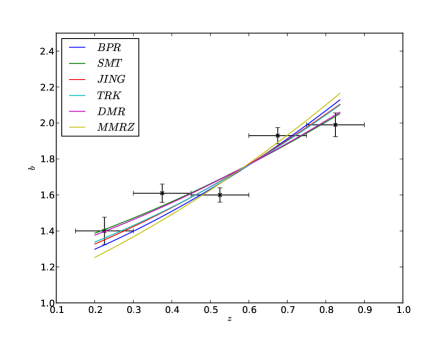
Figure 1: Comparison of the DESY1COSMO bias data with the bias models fits.

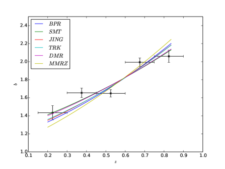
Figure 2: Comparison of the DES bias data scaled to the Planck (TT+lowP+lensing) priors with the bias models fits.

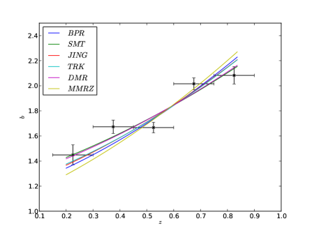
Figure 3: Comparison of the DES bias data scaled to DES/Planck/JLA/BAO priors with the bias models fits.

5 Comparison with LRGs from SDSS DR5

5.1 Angular Correlation Function Data

In this section we use the angular correlation function (ACF) of LRGs, already estimated in Sawangwit et. al. (2011), and compare it with the theoretical expectations of the $\Lambda$CDM model also incorporating the effects of the different bias models.

Specifically, we utilize the ACF of $\sim 655775$ photometrically selected LRGs from the SDSS DR5 catalogue with median redshift $z_{\star}=0.55$. This sample has been compiled using the same selection criteria as the 2dF-SDSS LRG and Quasar survey (hereafter 2SLAQ), which covers the redshift range $0.45<z<0.8$. Obviously, there is a substantially overlapping with the redshift range of the Dark Energy Survey, namely $0.15<z<0.9$. Based on the original work of Sawangwit et. al. (2011) we utilize the ACF up to an angular scale of $6000^{{}^{\prime\prime}}$ in order to avoid the effects of BAO’s. Since the goal of the present work is to test the performance of the most popular linear bias models we also exclude small angular scales ($\theta<140^{{}^{\prime\prime}}$, which translates to $<1\;h^{-1}$ Mpc at $z_{\star}$) and for which strong non-linear effects are expected. However, in our theoretical modeling we have taken into account a non-linear correction as far as the power spectrum is concerned the so called halo-fit model (see below). Notice, that the precise numerical values of the ACF data points with the corresponding errors can be found in Pouri et al. (2014), while for the total ACF data-set one may check the article of Sawangwit et. al. (2011).

5.2 Theoretical Angular Correlation Function

It is well known that the angular correlation function, $w(\theta)$ for small $\theta$’s is written as (cf. Basilakos & Plionis 2009 and references therein):

$$w(\theta)=\frac{1}{2\pi}\int_{0}^{\infty}k^{2}P(k)dk\int_{0}^{\infty}D^{2}(z)j(k,z,\theta)dz$$ (22)

with

$$j(k,z,\theta)=\frac{H_{o}}{c}\left(\frac{1}{N}\frac{dN}{dz}\right)^{2}b^{2}(z)E(z)J_{o}(k\theta x(z))\;,$$ (23)

where $x(z)$ is the comoving distance

$$x(z)=\frac{c}{H_{o}}\int_{0}^{z}\frac{dy}{E(y)}$$ (24)

and $J_{o}$ is the 0th order Bessel function of the first kind given by:

$$J_{0}(\omega)=\frac{1}{\pi}\int^{\pi}_{0}\cos(\omega sin\tau)d\tau$$ (25)

The quantity $1/N$ $dN/dz$ is the normalized source redshift distribution, estimated by the fitting formula of Pouri et. al. (2014)

$$\frac{dN}{dz}\propto\left(\frac{z}{z_{*}}\right)^{\alpha+2}e^{-(z/z_{*})^{\beta}}$$ (26)

with $(z_{\star},\alpha,\beta)=(0.55,-15.53,-8.03)$. For the power spectrum we are using the nonlinear power spectrum of Takashi et. al. (2011). Briefly, the latter approach consists the so called one-halo and two halo terms. The first one dominates at small scales, while the second one plays a key role at large scales.

5.3 Fitting models to the LRGs SDSS DR5 ACF data

In order to quantify the free parameters of the models we perform a $\chi^{2}$-minimization procedure and compare the measured LRG angular correlation function of Sawangwit et al. (2011) with the expected theoretical ACF given by Eq.(22). In examining the model dependence we restrict our analysis to flat $\Lambda$CDM with $n=0.9671$, $\Omega_{b}=0.0484$ (Spergel et al. 2015) and vary $\Omega_{m}h$ and $M_{h}$. Also, in order to treat the $\sigma_{8}-\Omega_{m}$ relation we use the following parametrization $\sigma_{8}=0.818(0.3/\Omega_{m})^{0.26}$ (Spergel et al. 2015). Therefore, the $\chi^{2}$ function is defined as:

$$\chi^{2}=\displaystyle\sum^{11}_{i=1}\left[\frac{w_{obs}(\theta_{i})-w_{th}(\theta_{i},\textbf{p})}{\sigma_{w,i}}\right]^{2}$$ (27)

where $\sigma_{w,i}$ is the uncertainty of the observed ACF (see Table 1 in Pouri et al. 2014). Here the statistical vector ${\bf p}$ contains two independent free parameters, namely ${\bf p}=(\Omega_{m}h,M_{h})$.

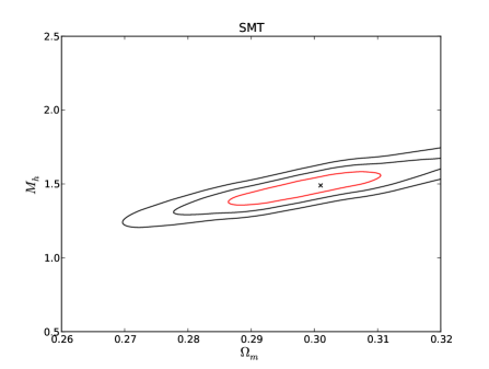
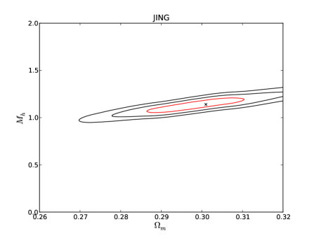
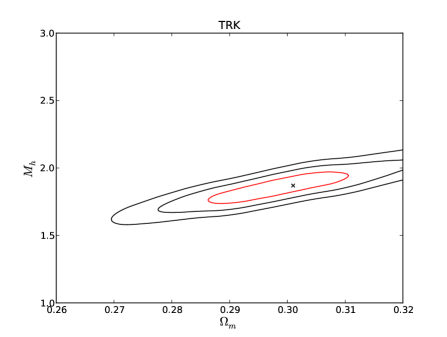
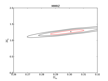
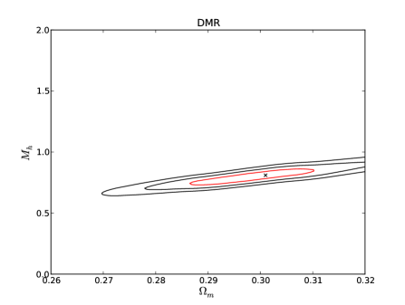
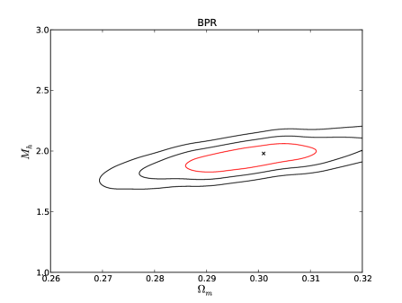
Figure 4: Contour plot of the two fitted parameters, halo mass, $M_{h}$ and $\Omega_{m}$ for the indicated bias models. The $1\sigma$ level is indicated by the red curve.

In Table 3 we present the best fit $(\Omega_{m}h,M_{h})$ parameters for the different models and as it can be seen, the fit to the data, as indicated by the value of the $\chi^{2}_{min}$, is equally good for all models, i.e., $\chi^{2}_{min}\simeq 7.1$ (with AIC${}_{c}\simeq 10.43$) for 9 degrees of freedom for all models. The first interesting result, as can be seen from the Table 3, is that for all bias models the likelihood analysis peaks at $\Omega_{m}h=0.204\pm 0.0075$ which reduces to $\Omega_{m}=0.30\pm 0.01$ for $h=0.678$. Notice, that the latter value is in excellent agreement with that of Planck (TT+lowP+lensing; Ade et al. 2016), of DES/Planck/JLA/BAO (Abbott et al. 2017) and the re-analysis of the Planck data provided by Spergel et al. (2015). Using the Planck value of the Hubble constant $H_{0}=67.8$km/s/Mpc, provided by Spergel et al. (2015), in Figure 4 we present the 1$\sigma$, 2$\sigma$ and $3\sigma$ contours in the $(\Omega_{m},M_{h})$ plane for the SMT, JING, TRK, MMRZ, DMR and BPR bias models, respectively.

The second result worth mentioning is that the fitted DM halo mass is somewhat larger with respect to that of the DES data, namely it ranges between $\sim 0.8\times 10^{13}h^{-1}M_{\odot}$ and $\sim 2\times 10^{13}h^{-1}M_{\odot}$. The corresponding weighted mean and the combined weighted standard deviation of the DM halo mass are:

$${\bar{M}}_{h}=1.426(\pm 0.405)\times 10^{13}h^{-1}M_{\odot}$$

As we have already found previously using the DES bias data, also here the weighted mean DM halo mass tends to that of SMT.

The latter results, concerning the weighted mean DM halo mass, although based on the integrated clustering of LRGs in one overall redshift bin, are consistent, within one standard deviation, to those of Section 4. This should have been expected since both surveys (DES and 2SLAQ) trace the same extragalactic objects (LRGs) in a similar redshift range. Furthermore, using the TRK bias model we find now that the derived DM halo mass is consistent at $\sim 2\sigma$ level with that of Sawangwit et al. (2011), namely $M_{h}\simeq 2(\pm 0.1)\times 10^{13}h^{-1}M_{\odot}$ (see also Pouri et al. 2014). Notice, that the latter holds for the BPR bias model in the case of DES/Planck/JLA/BAO rescaled bias data. Sawangwit et al. (2011) used the bias model of Sheth et al. (2001) together with the revised parameters of Tinker et al. (2005). Using these parameters for the SMT model in our analysis we obtain $M_{h}=2.24(\pm 0.1)\times 10^{13}h^{-1}M_{\odot}$.

Lastly, we verify that perturbations around the values $h=0.678$, $n=0.9671$ and $\Omega_{b}=0.0484$ do not really affect the aforementioned statistical results.

In Figure 5, we plot the observed $w(\theta)$ for the 2SLAQ LRGs, with the best fit model of the angular correlation function provided by Eq.(22) and the minimization procedure presented above. Notice, that the solid curve corresponds to the bias model of SMT with $\Omega_{m}=0.301$ and $M_{h}=1.495\times 10^{13}h^{-1}M_{\odot}$. The red stars indicate the ACF data in the range $0<\theta<140^{{}^{\prime\prime}}$, which as we have already mentioned in section 5.1 have been excluded from our analysis in order to avoid the strong non-linear effects. We remind the reader that these scales, at the median redshift of $z_{\star}=0.55$, correspond to spatial separations $\lesssim 1h^{-1}{\rm Mpc}$.

Bias Model	$10^{13}h^{-1}M_{\odot}$	$\Omega_{m}h$	$\chi^{2}_{min}/d.o.f.$
SMT	$1.495^{+0.075}_{-0.060}$	$0.204\pm 0.0068$	$7.05$
JING	$1.155^{+0.060}_{-0.040}$	$0.204\pm 0.0075$	$7.05$
TRK	$1.880^{+0.090}_{-0.060}$	$0.204\pm 0.0075$	$7.05$
MMRZ	$1.270^{+0.070}_{-0.035}$	$0.204\pm 0.0075$	$7.06$
DMR	$0.810^{+0.045}_{-0.030}$	$0.204\pm 0.0075$	$7.05$
BPR	$1.945^{+0.085}_{-0.115}$	$0.204\pm 0.0075$	$7.05$

Table 3: Results of the $\chi^{2}$ minimization procedure using the LRGs ACF of 2SLAQ (see Sawangwit et al. 2011 and Table 1 in Pouri et al. 2014). In this case we have $\Delta$AIC $\simeq 0$.

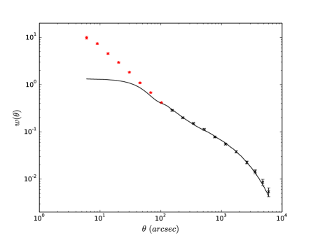
Figure 5: Comparison between the predicted angular correlation function for the BPR bias model (solid line) and the LRGs correlation function data points of Sawangwit et al. (2011) (by red stars we indicate the non-linear scales: $0<\theta\leq 140^{{}^{\prime\prime}}$). The solid curve corresponds to the $\Lambda$CDM model expectations using the SMT bias model with $\Omega_{m}=0.301$ and $M_{h}=1.495\times 10^{13}h^{-1}M_{\odot}$.

6 Conclusions

In this work we have used the bias data of Luminous Red Galaxies, recently released by the Dark Energy Survey (DES) team, in order to investigate the ability of six bias evolutions models to represent the observational data. Implementing a standard $\chi^{2}$ minimization procedure between the models and the data we have placed tight constraints on the only free parameter of the model, namely the dark matter halo mass $M_{h}$. Based on the best-$\chi^{2}$ and the value of the Akaike information criterion we found that most bias models fit equally well the DES bias data. The intrinsic differences of the bias models appear to be absorbed in the fitted value of the dark-matter halo mass in which LRGs live, and which ranges between $\sim 6\times 10^{12}h^{-1}M_{\odot}$ and $1.4\times 10^{13}h^{-1}M_{\odot}$ for the different bias models.

The bias model that best fit the DES bias data is that of Sheth et al. (2001), while we found indications for a tension between the model of Ma et. al. (2011) and the bias data. Moreover, we have shown that the Jing (1998), Tinker et. al. (2010), Ma et al. (2011) and the Basilakos et al. (2011) bias models predict consistent values (within $1\sigma$) of the mass of dark matter halos hosting LRGs with that of Sheth et al. (2001). We have also found that regardless the value of the fitted DM halo mass, the bias model of Sheth et al. (2001) is statistically equivalent to those of Jing (1998), Tinker et. al. (2010) and de Simone et. al. (2011), since $|\Delta$AIC$|\leq 2$.

In the second part of the paper we have used again a standard $\chi^{2}$ minimization procedure between the theoretical angular clustering models, which also include the evolution of bias, and the corresponding 2SLAQ LRG clustering. This analysis also has showed that the bias models explored are statistically equivalent. Furthermore, it provided a value of $\Omega_{m}=0.30\pm 0.01$, which is in excellent agreement with that of Planck (TT+lowP+lensing; Ade et al. (2016), DES/Planck/JLA/BAO (Abbott et al. 2017) and the reanalysis of the Planck data (Spergel et al. 2015). Finally, concerning the estimated DM halo mass, the clustering analysis has provided a range between $8\times 10^{12}h^{-1}{\rm Mpc}\lesssim M_{h}\lesssim 2\times 10^{13}h^{-1}M_{\odot}$, results which are somewhat larger with those based on the DES bias data. However, using an inverse-AIC_c weighting we find that the model average value of the DM halo mass that hosts LRGs are consistent within 1$\sigma$ using either the DES or the SDSS 2SLAQ analyses.

References

- [Abbott et al. 2017] Abbott, T. M. C., arXiv:1708.0153
- [Ade et al. 2016] Ade, P. A. R. 2016, A&A, 594A, 1P (Plank data)
- [Akaike 1974] Akaike, H., 1974, IEEE Transactions of Automatic Control, 1 9, 716
- [Assassi et. al. 2012] Assassi, V., Baumann, D., Green, D., Zaldarriaga, M. 2014, JCAP, 08, 056A
- [Baldauf et. al. 2012] Baldauf, T., Seljak, U., Desjacques, V., McDonald, P., 2012, Phys. Rev. D, 86, 3540
- [Bagla 1998] Bagla, J. S. 1998, MNRAS, 299, 417
- [Bardeen et al. 1986] Bardeen, J. M., Bond, J. R., Kaiser, N., Szalay, A. S. 1986, ApJ, 304, 15
- [Basilakos & Plionis 2001] Basilakos, S., Plionis, M. 2001, ApJ, 550, 522
- [Basilakos 2001] Basilakos S., 2001, MNRAS, 326, 203
- [2003] Basilakos, S., & Plionis, M. 2003, ApJ, 593, L61
- [Basilakos and Plionis 2005] Basilakos S. & M. Plionis, 2005, MNRAS, 360, L35
- [Basilakos and Plionis 2006] Basilakos S. & M. Plionis, 2006, ApJL, 650, L1
- [Basilakos and Plionis 2009] Basilakos S. & M. Plionis, 2009, MNRAS, 400, L57
- [Basilakos and Plionis 2010] Basilakos S. & M. Plionis, 2010, ApJL, 714, L185
- [Basilakos, Plionis & Figueroa 2008] Basilakos, S., Plionis, M., Ragone-Figueora, C. R. 2008, ApJ, 678, 627
- [Basilakos, Plionis & Pouri 2011] Basilakos, S., Plionis, M., Pouri, A. 2011, Phys. Rev. D, 83, 123525
- [Basilakos et al. 2012] Basilakos, S., Dent, J. B., Dutta, S., Perivolaropoulos, L., Plionis, M., 2012, Phys. Rev. D, 85, 123501
- [Bel et. al. 2015] Bel, J., Hoffmann, K., Gaztanaga, E., 2015, MNRAS, 453, 259
- [Hoffmann et. al. 2017] Hoffmann, K., Bel, J., Gaztanaga, E., 2017, MNRAS, 465, 2225
- [Hoffmann et. al. 2015] Hoffmann, K., Bel, J., Gaztanaga, E., 2015, MNRAS, 450, 1674
- [Burnham and Anderson 2002] Burnham K. P., Anderson D. R., 2002, Model Selection and Multimodel Inference, 2nd edn. Springer-Verlag, New York
- [Burnham and Anderson 2004] Burnham K. P., Anderson D. R., 2004, Sociol. Method. Res., 33, 261
- [Chan, Scoccimarro & Sheth 2012] Chan, K. C., Scoccimarro, R., Sheth, R, K., 2012, Phys. Rev. D, 85, 3509
- [Catelan] Catelan P., Lucchin F., Matarrese S., Porciani C., 1998, MNRAS, 297,692
- [Cole & Kaiser 1989] Cole, S., Kaiser, N. 1989, MNRAS, 237, 1127
- [de Simone et al. 2011] de Simone, A., Maggiore, M., Riotto, A. 2011, MNRAS, 412, 2587
- [DES Collaboration 2017] DES Collaboration, 2017, arXiv:1708.01530v[astro-ph.CO]
- [Desjacques et al. 2016] Desjacques, V., Donghui, J., Schmidt, F. 2016, arXiv161109787D
- [Di Porto et al. 2016] Di Porto, C., et al. 2016, A&A, 594, 62
- [Eisenstein et al. (2001)] Eisenstein, D. J., et al. 2001, AJ, 122, 2267
- [Eisenstein & Hu 1998] Eisenstein, D. J., Hu, W. 1998, ApJ, 496, 605
- [Elvin-Poole et al. 2017] Elvin-Poole, M. et al. 2017, arXiv:1708.01536v[astro-ph.CO] (DES Y1COSMO)
- [Fry 1996] Fry, J. N. 1996, ApJ, 461, L65
- [Fr] ry, J. N. & Gaztanaga, E. 1993, ApJ 413, 447
- [Hamilton 1998] Hamilton, A. J. S. 1998, Linear Redshift Distortions: A Review. Kluwer, Dordrecht, p. 185
- [Hui & Parfrey 2008] Hui, L., Parfrey, K. P. 2008, Phys. Rev. D, 77, 043527
- [Inoue & Takahashi 2012] Inoue, K. T., Takahashi, R. 2012, MNRAS, 426, 2978
- [Jing 1998] Jing, Y. P. 1998, ApJ, 503, L9
- [Kaiser 1984] Kaiser, N. 1984, ApJ, 284, L9
- [Kaiser (1987)] Kaiser, N. 1987, MNRAS, 227, 1
- [Kraise et. al. (2017)] Krause, E., et al. (DES Collaboration), submitted to Phys. Rev. D (2017), arXiv:1706.09359 [astro-ph.CO]
- [Lazeyras (2016)] Lazeyras, T., Wagner, C., Baldauf, T., Schmidt, F. 2016, JCAP, 02, 018L
- [Liddle (2007)] Liddle A. R., 2007, MNRAS, 377, L74
- [Ma et al. 2011] Ma, C.-P., Maggiore, M., Riotto, A., Jun, Z. 2011, MNRAS, 411, 2644
- [Maggiore et. al. 2010a, b, c] Maggiore, M. & Riotto, A. 2011, ApJ, 711, 907
- [Maggiore] Maggiore, M. & Riotto, A. 2011, ApJ, 717, 515
- [Ma] Maggiore, M. & Riotto, A. 2011, ApJ, 717, 526
- [Marinoni et al. 2005] Marinoni, C., et al. 2005, A&A, 442, 801
- [Matarrese et al. 1997] Matarrese, S., Coles, P., Lucchin, F., Moscardini, L. 1997, MNRAS, 286, 115
- [Matsubara 2004] Matsubara T., 2004, ApJ, 615,573
- [McDonald et. al. 2009] cDonald, P. & Roy, A., JCAP 0908, 020 (2009), 0902.0991.
- [Mo & White 1996] Mo, H. J., White, S. D. M. 1996, MNRAS, 282, 347
- [Moscardini et al. 1998] Moscardini, L., Coles, P., Lucchin, F., Matarrese, S. 1998, MNRAS, 299, 95
- [Nusser & Davis 1994] Nusser, A., Davis, M. 1994, ApJ 421, L1
- [Papageorgiou et al. 2012] Papageorgiou, A., Plionis, M., Basilakos, S., Ragone-Figueroa, C. 2012, MNRAS, 422, 106P
- [Paranjape et al. 2013] Paranjape, A. et al. 2013, MNRAS, 436, 449P
- [Paranjape et al. 2013] Paranjape, A., Sheth, R. K., Desjacques, V. 2013, MNRAS, 431, 1503P
- [Peebles 1980] Peebles, P. J. E. 1980, The Large-scale Structure of the Universe. Princeton University Press, Princeton
- [Pouri et al. 2014] Pouri, A., Basilakos, S., Plionis, M. 2014, JCAP, 08, 042
- [Sawangwit et al. (2011)] Sawangwit, U., et al. 2011, MNRAS, 416, 3033
- [Schaefer, Douspis & Aghanim 2009] Schaefer, B. M., Douspis, M., Aghanim, N. 2009, MNRAS, 397, 925
- [Sheth & Tormen 1999] Sheth, R. K., Tormen, G. 1999, MNRAS, 308, 119
- [Sheth, Mo & Tormen 2001] Sheth, R. K., Mo, H. J., Tormen, G. 2001 MNRAS, 323, 1
- [Smith et al. (2003)] Smith, R. E., Peacock, J. A., et al. 2003, MNRAS, 341, 1311
- [Spergel et al. 2015] Spergel, D. N., Flauger, R., Hlozek, R. 2015, PhRvD, 91b3518S
- [Sugiyama 1995] Sugiyama, N. 1995, ApJ, 100, 281
- [Sugiura 1978] Sugiura, N. 1978, Communications in Statistics A, Theory & Methods, 7, 13
- [Takahashi et al. (2012)] Takahashi, R., et al. 2012, ApJ, 761, 152
- [Takahashi et al. 2011] Takahashi, R., et al. 2011, ApJ, 742, 15
- [Tegmark & Peebles 1998] Tegmark, M., Peebles, P. J. E. 1998, ApJ, 500, L79
- [Tinker et al. 2005] Tinker, J. L., Weinberg, D. H., Zheng, Z. 2005, ApJ, 631, 41
- [Tinker et al. 2010] Tinker, j. L., et al. 2010, ApJ, 724, 878
- [Valageas 2009] Valageas, P. 2009, A&A, 508, 93
- [2011] Valageas, P. 2009, A&A, 525, 98
- [Valageas & Nishimichi 2011] Valageas, P., Nishimichi, T. 2011, A&A, 527, A87
- [Weinberg & Kamionkowski 2003] Weinberg, N. N., Kamionkowski, M. 2003, MNRAS, 341, 251