Network Model Selection Using Task-Focused Minimum Description Length

Abstract.

Networks are fundamental models for data used in practically every application domain. In most instances, several implicit or explicit choices about the network definition impact the translation of underlying data to a network representation, and the subsequent question(s) about the underlying system being represented. Users of downstream network data may not even be aware of these choices or their impacts. We propose a task-focused network model selection methodology which addresses several key challenges. Our approach constructs network models from underlying data and uses minimum description length (MDL) criteria for selection. Our methodology measures efficiency, a general and comparable measure of the network’s performance of a local (i.e. node-level) predictive task of interest. Selection on efficiency favors parsimonious (e.g. sparse) models to avoid overfitting and can be applied across arbitrary tasks and representations. We show stability, sensitivity, and significance testing in our methodology.

1. Introduction

Networks are fundamental models for data used in practically every application domain. In most instances, several implicit or explicit choices about the network definition impact the translation of underlying data to a network representation, and the subsequent question(s) about the underlying system being represented. Users of downstream network data may not even be aware of these choices or their impacts. Do these choices yield a model which is actually predictive of the underlying system? Can we discover better (i.e. more predictive, simpler) models?

A network derived from some data is often assumed to be a true representation of the underlying system. This assumption introduces several challenges. First, these relationships may be very time-dependent: an aggregation of edges might not reflect the behavior of the underlying system at any time (Caceres and Berger-Wolf, 2013). Second, relationships may be context-dependent: where the same network inferred from data predicts one behavior of the system but not another (Brugere et al., 2017b). Any subsequent measurement on the network (e.g. degree distribution, diameter, clustering coefficient, graph kernels) treats all edges equally, when a path or community in the network may only be an error of aggregation.

Task-based network model selection addresses the latter challenge by comparing multiple representations for predicting a particular behavior (or context) of interest. In this context, the network is a space which structures a local predictive task (e.g. “my neighbors are most predictive of my behavior”), and model selection reports the best structure.

Work in network model selection has typically focused on inferring parameters of generative models from a given network, according to some structural or spectral features (e.g. degree distribution, eigenvalues) (Takahashi et al., 2012). However, preliminary work has extended model selection to criteria on task performance with respect to generative models for a given network (Caceres et al., 2016), and methodologies representing underlying data as networks (Brugere et al., 2017b).

We propose a task-focused network model selection methodology which addresses several key challenges. Our approach constructs network models from underlying data and uses minimum description length (MDL) criteria for selection. Our methodology measures efficiency, a general and comparable measure of the network’s performance of a local (i.e. node-level) predictive task of interest. Selection on efficiency favors parsimonious (e.g. sparse) models to avoid overfitting and can be applied across arbitrary tasks and representations. We show stability, sensitivity, and significance testing in our methodology.

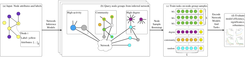
Figure 1. A high-level overview of our methodology. (a) Given as input: nodes with associated attribute and label data, potential network structure(s) are optionally provided (dashed lines). We use network inference models to construct multiple networks from data (note: stack of models). (b) On each network model, for each node ‘$i$’, we sample nodes (shown by node color) and their associated attributes and labels, according to different sample methods and node characterization heuristics (e.g. ‘high degree’, ‘high activity’). (c) we generate ‘$b$’ samples by each method at varying sample size $k$, each row is a trained task model (e.g. random forest) to predict label ‘$i$’ (‘yellow’) given sampled attribute data and labels. (d) we encode each collection of task models from (c) and network representation from (b) to measure the most efficient model for performing the task, and select that network representation.

1.1. Related work

Our work is related to network structure inference (Brugere et al., 2016; Kolaczyk, 2009). This area of work constructs a network model representation for attributes collected from sensors, online user trajectories or other underlying data. Previous work has focused on these network representations as models of local predictive tasks, performed on groups of entities, such as label inference (Namata et al., 2015) and link prediction (Hasan and Zaki, 2011; Liben-Nowell and Kleinberg, 2007). A ‘good’ network in this setting is one which performs the task well, under some measure of robustness, cost, or stability. Previous work examined model selection under varying network models, single or multiple tasks, and varying task methods (Brugere et al., 2017a, b).

The minimum description length (MDL) principle (Rissanen, 2004) measures the representation of an object or a model by its smallest possible encoding size in bytes. This principle is used for model selection for predictive models, including regression (Hansen and Yu, 2001) and classification (Mehta et al., 1996). MDL methods have also been applied for model selection of data representations including clusterings, time series (Hu et al., 2011; Hansen and Yu, 2001), networks (Zhao et al., 2006) and network summarization (Koutra et al., 2014). MDL has been used for structural outlier and change detection in dynamic networks (Ferlez et al., 2008; Sun et al., 2007). Our methodology encodes a collection of predictive models, together with the underlying network representation for model selection. No known work encodes both of these objects for model selection.

Several generative models exist to model correlations between attributes, labels, and network structure, including the the Attributed Graph Model (AGM) (Pfeiffer III et al., 2014), and Multiplicative Attribute Graph model (MAG) (Kim and Leskovec, 2012). These models are additive to our methodology, and could be applied and evaluated as potential models within our methodology.

Our work is orthogonal to graph kernels (Vishwanathan et al., 2010) and graph embeddings (Hamilton et al., 2017). These methods traverse network structure to extract path features and represent nodes in a low-dimensional space, or to compare nodes/graphs by shared structural features. We treat this graph traversal as one possible query of nodes for input to local tasks, but do not compare graphs or nodes directly; our focus is to evaluate how well the fixed model performs the local task over all nodes.

1.2. Contributions

We formulate a task-focused model selection methodology for networks.

• Model selection methodology: We propose a generalized approach for evaluating networks over arbitrary data representations for performing particular tasks.

• Network efficiency: We propose a general minimum description length (MDL) efficiency measure on the encoding of network representations and task models, which is comparable over varying models and datasets,

• Validation and significance We empirically demonstrate stability, sensitivity, and significance testing of our model selection methodology.

2. Methods

Figure 1 gives a schematic overview of our model selection methodology. In Figure 1(a) as input, we are given attribute-set $A$ and label-set $L$ associated with entities $i\in V$. Labels are a notational convenience to denote an attribute of interest for some predictive task (e.g. label inference, link prediction). We may be given a network topology (dashed lines), which we treat as one possible network model in the evaluation.

We apply a collection of network inference methods to generate separate network topologies. In Figure 1(b), for each network topology, we use several network sampling methods to sample attribute and label data for input to a supervised classification/regression task. Boxes indicate different node characterization heuristics which can be sampled: ‘high degree’, ‘high activity’, or ‘communities’. Node colors indicate one sample from each of sampling method with respect to node $i$: green nodes denote a local, orange nodes denote a community sample (the same node in two samples indicated by two-color nodes). Purple is a sample of high-degree nodes. Blue represents a sample of high-activity nodes (e.g users with the most interactions, most purchases, most ratings), and cyan represents a random sample of nodes.

In Figure 1(c), each network sample method produces samples of length $k$, and is repeatedly sampled to create $b$ supervised classification instances per method. Each row corresponds to a supervised classification task trained on attributes and labels in the sample, to predict the label of $i$ (e.g. ‘yellow’). Finally, in Figure 1(d), we encode the predictive models (e.g. the coefficients of an SVM hyper-plane or random forest trees) and the network in an efficient byte-string representation, and evaluate the best model using minimum description length (MDL) criteria. We propose a general and interpretable measure of efficiency for solving our task of interest, and show stability and significance testing over our collection of models.

2.1. Preliminaries and notation

Let $V=\{1...,i...,n\}$ be a set of entities to which we refer to as ‘nodes.’ Let $A=\{\vec{a}_{i}\}$ be a set of attribute-vectors and $L=\{l_{i}\}$ be a set of target labels of interest to be learned, where $i\in V$. Let $\mathcal{Q}:V\times\mathbf{Z}^{+}\times(\mbox{other data})\to V^{k}$ be a network query function (see the full definition below) that produces query-sets of nodes $S\subseteq V$ of a given size $k$. Let $\mathcal{C}:A\times L\times V\to L$ be a classifier trained on attributes and labels of a node subset $S$ to produce a prediction $l^{\prime}_{i}$, for node $i$.

2.2. Network query functions

In our methodology, we access the network for our given objective using a network query function on node $i$, which returns a set of nodes of arbitrary size subject to the network topology and function definition.

To compare different query functions under similar output, we introduce a bounded query of size $k$. With an input of node $i$ and search size $k$, bounded network query function $\mathcal{Q}$ outputs a set of unique nodes:

(1) $$\mathcal{Q}(i,k)\rightarrow\{j_{1},j_{2},...,j_{k}\},\text{ where }i\notin\{j_{1},...,j_{k}\}$$

In general, these queries sample from the possible node-sets, yielding different result-set samples on a repeated input $i$. We measure these functions over a distribution of node-set samples, with replacement, analogous to the bootstrap sample (Efron and Tibshirani, 1993).

Network adjacency is one such query method, which randomly samples from ${\mathcal{N}(i)\choose k}$ subsets, with replacement. Breadth-first search $\mathcal{Q}_{\texttt{bfs}}(i,k,E)$ generalizes adjacency to higher-order neighbors, where nodes in the farthest level is selected at random. Over varying query size $k$, breadth-first search is well-suited for measuring the performance of the network in finding relevant nodes ‘nearer’ to the query.

While $\mathcal{Q}$ may sample an underlying network edge-set $E$, our methodology evaluates any network query function, regardless of underlying implementation. In geometric space, $\mathcal{Q}_{l_{2}}$ may sample nodes in increasing Euclidean distance from $i$. Query heuristics can also be derived from the attribute-set $A$. For example, $\mathcal{Q}_{\texttt{activity-net}}(i,k,A)$ (defined below) may query points by the number of non-zero attributes or some other attribute function, and sample according to some similarity to $i$.

2.2.1. Network efficiency

We evaluate each network query function according to a minimum description length (MDL) criterion. We repeatedly sample $\mathcal{Q}_{r}(i,k)$ ($r$ for ‘rule’), to construct $b$ samples of attribute vectors and labels, of size $k$. We train each classifier $\mathcal{C}(A[S],L[S])$ from these attribute and label data. Let $C_{r}[i,k]$ be the resulting set of trained classifiers:

(2) $$C_{r}[i,k]=\{\mathcal{C}(A[\mathcal{Q}_{r}(i,k)_{1}],L[\mathcal{Q}_{r}(i,k)_{1}]),...$$

$$\mathcal{C}(A[\mathcal{Q}_{r}(i,k)_{b}],L[\mathcal{Q}_{r}(i,k)_{b}])\}_{|b|}$$

Let $\operatorname*{correct}(C_{r}[i,k])$ be the sum of correct predictions of the $b$ task classifiers on test input $\mathcal{C}_{r}(\vec{a_{i}},l_{i})$.

Definition 2.1.

The efficiency of a network query function $\mathcal{Q}_{r}$ with respect to a node $i$ is the number of correct predictions per byte (higher is better). The efficiency $\mathcal{E}$ is the maximum given by the value of $k$ which yields the maximum of correct predictions divided by the median encoding cost, both aggregates of $b$ samples:

(3) $$\mathcal{E}(\mathcal{Q}_{r},i)=\max_{k}\left\{{\frac{\operatorname*{correct}(C_{r}[i,k])}{\operatorname*{med}_{b}(\operatorname*{bytes}(C_{r}[i,k]))}}\right\}.$$

Let $\kappa_{i}=\operatorname*{argmax}_{k}\mathcal{E}(\mathcal{Q}_{r},i)$, the $k$ associated with the maximum efficiency of node $i$. We then sum $\operatorname*{bytes}(\mathcal{C}_{r}[i,\kappa_{i}])$ and $\operatorname*{correct}(\mathcal{C}_{r}[i,\kappa_{i}])$ over all $i$ to get efficiency over task models trained on samples from $\mathcal{Q}_{r}$. We also encode $\mathcal{Q}_{r}$ and measure its representation cost:

(4) $$\begin{split}\operatorname*{correct}(\mathcal{C}_{r}){}=\sum_{i}\operatorname*{correct}(\mathcal{C}_{r}[i,\kappa_{i}])\\ \operatorname*{bytes}(\mathcal{C}_{r}){}=\sum_{i}\operatorname*{bytes}(\mathcal{C}_{r}[i,\kappa_{i}])\end{split}$$

Then, the overall efficiency of $\mathcal{Q}_{r}$ is given by:

(5) $$\mathcal{E}(\mathcal{Q}_{r})=\frac{\operatorname*{correct}(\mathcal{C}_{r})}{\operatorname*{bytes}(\mathcal{C}_{r})+\operatorname*{bytes}(\mathcal{Q}_{r})}.$$

Encoding the function $\mathcal{Q}_{r}$ favors parsimonious models and avoids overfitting the representation to evaluation criteria such as accuracy or precision. However, such encoding requires careful consideration of the underlying representation, which we cover in Section 2.4.1. Omitting the encoding cost of $\mathcal{Q}_{r}$ in Equation 5 measures only the extent to which the network query function trains ‘good’ task models in its top-$k$ samples. This is suitable if we are not concerned with the structure of the underlying representation, such as its sparsity. To favor interpretability of efficiency in real units (correct/byte), we avoid weight factors for the terms in the efficiency definition. However, in practice this would provide more flexibility to constrain one of these criteria.

2.3. Problem statement

We can now formally define our model selection problem, including inputs and outputs:

Given: A set of nodes $V$, Node Attribute-set $A$, Node Label-set $L$, Network query function-set $Q=\{\mathcal{Q}_{r}\}$, where $\mathcal{Q}_{r}(i,k)\rightarrow\{v_{j_{1}},v_{j_{2}},...v_{j_{k}}\}$, Task $\mathcal{C}$, where $\mathcal{C}(A[S],L[S],\vec{a}_{i})\rightarrow l^{\prime}_{i}$

Select: Network query function $\mathcal{Q}^{\prime}\in Q$

Where: $\mathcal{Q}^{\prime}=\operatorname*{argmax}_{r}\mathcal{E}(\mathcal{Q}_{r})$

Problem 1 MDL Task-Focused Network Inference Model Selection

For brevity, we refer to ‘model selection’ simply as selecting the network representation and its associated network query function for our task of interest. The underlying query functions in set $Q$ may be implemented as arbitrary representations which can be randomly sampled (e.g. lists). This model selection methodology measures, for example whether a network is a better model than other non-network sampling heuristics, group-level sampling (e.g. communities), etc. accounting for representation cost of each. That is, whether a network is necessary in the first place. As a consequence, we may select a different queried representation than a network.

Previous work has evaluated network model-selection for robustness to multiple tasks (e.g. link prediction, label prediction) as well as different underlying task models (e.g. random forests, support vector machines) (Brugere et al., 2017b). Problem Problem 1 can straightforwardly select over varying underlying network models, tasks, or task models which maximize efficiency. We simplify the selection criteria to focus on measuring the efficiency of network query functions and their underlying representations, but this current work is complimentary to evaluating over larger parameter-spaces and model-spaces.

2.4. Network models

We define several networks queried by network query functions $\mathcal{Q}_{r}$. Our focus is not to propose a novel network inference model from attribute and label data (see: (Pfeiffer III et al., 2014; Kim and Leskovec, 2012)). Instead we apply existing common and interpretable network models to demonstrate our framework. The efficiency of any novel network inference model should be evaluated against these baselines.

A network model $\mathcal{M}$ constructs an edge-set from node attributes and/or labels: $\mathcal{M}_{j}:\mathcal{M}_{j}(A,L)\rightarrow E_{j}$. We use simple $k$-nearest neighbor (KNN) and Threshold (TH) models common in many domains.

Given a similarity measure $\mathrm{d}(\vec{a}_{i},\vec{a}_{j})\rightarrow s_{ij}$ and a target edge count $\rho$, this measure is used to produces a pairwise attribute similarity space. We select edges by:

• $k$-nearest neighbor $\mathcal{M}_{\texttt{KNN}}(A,\mathrm{d}(),\rho)$: for a fixed $i$, select the top $\lfloor{\frac{\rho}{|V|}}\rfloor$ most similar $\mathrm{d}(\vec{a}_{i},\{A\setminus\vec{a}_{i}\})$. In directed networks, this produces a network which is $k$-regular in out-degree, with $k=\lfloor{\frac{\rho}{|V|}}\rfloor$.

• Threshold $\mathcal{M}_{\texttt{TH}}(A,\mathrm{d}(),\rho)$: over all pairs $(i,j)\in V$ select the top $\rho$ most similar $\mathrm{d}(\vec{a}_{i},\vec{a}_{j})$.

Let these edge-sets be denoted $E_{\texttt{KNN}}$ and $E_{\texttt{TH}}$, respectively. We use varying network sparsity ($\rho$) on these network models to choose ‘sparse’ or ‘dense’ models. Similarity measures may vary greatly by application. In our context, attribute data are counts and numeric ratings of items (e.g. films, music artists) per user. We use a sum of intersections (unnormalized), which favors higher activity and does not penalize mismatches:

(6) $$\mathrm{d}_{INT}(\vec{a}_{i},\vec{a}_{j})=\sum\nolimits_{l}\mathrm{min}(a_{il},a_{jl})$$

2.4.1. Encoding networks and tasks

Table 1 summarizes the network query functions (Equation 1) used in our methodology, and their inputs. We define only a small number of possible functions, focusing on an interpretable set which helps characterizes the underlying data. The encoding cost increases from top to bottom.

activity-top and degree-top are the simplest network query functions we define. activity-top sorts nodes by ‘activity’, i.e. the number of non-zero attributes in $\vec{a}_{i}$, and selects the top-$\ell$ ranked nodes ($\ell<<|V|$). An ordering is generated by random sub-sampling of this list. degree-top does similar on node degree with respect to some input $E$.

cluster applies graph clustering (i.e. community detection) on the input edge-set $E$. This reduces the network to a collection of lists representing community affiliation. Each node is affiliated with at most one community label. Although both degree-top and cluster are derived from an underlying network, we only encode the reduced representation. This is by design, to measure whether the network is better represented by a simple ranking function which we represent in $\mathcal{O}(\ell)$ space, a collection of groups in $\mathcal{O}(|V|)$ space, or edges in $\mathcal{O}(|E|)$ space. random produces random node subset, encoded in $\mathcal{O}(|V|)$ space.

bfs is a breadth-first search of an underlying edge-set $E$ from seed $i$. This is encoded by an adjacency list (a list of lists), in $\mathcal{O}(|E|)$. degree-net is an ad-hoc network with all out-edges to some node in the top-$\ell$ nodes of degree-top. For each node $i$, we select $m<\ell$ most similar nodes and define out-edges from $i$. This is a KNN graph, where $k=m$, constrained to high-degree nodes. This additional encoding cost relative to degree-top measures the extent that specialization exists in the top-ranked individuals as a set of task ‘exemplars’ for all nodes. activity-net is defined analogously with respect to activity-top.

Network Query Function	Encoding
$\mathcal{Q}_{\texttt{activity-top}}(i,k,\mathrm{sort}(A),\ell)$	$\mathcal{O}(\ell)$
$\mathcal{Q}_{\texttt{degree-top}}(i,k,\mathrm{sort}(E),\ell)$	$\mathcal{O}(\ell)$
$\mathcal{Q}_{\texttt{cluster}}(i,k,\mathrm{cluster}(E))$	$\mathcal{O}(|V|)$
$\mathcal{Q}_{\texttt{random}}(i,k,V)$	$\mathcal{O}(|V|)$
$\mathcal{Q}_{\texttt{bfs}}(i,k,E)$	$\mathcal{O}(|E|)$
$\mathcal{Q}_{\texttt{activity-net}}(i,k,\mathrm{sort}(A),m,\ell)$	$\mathcal{O}(|V|\times m)$
$\mathcal{Q}_{\texttt{degree-net}}(i,k,\mathrm{sort}(E),m,\ell)$	$\mathcal{O}(|V|\times m)$

Table 1. The input signature and space complexity of network query functions. We define four functions implemented by non-network structures (top), and three implemented by a network (bottom)

To demonstrate our methodology, we use Random Forest task models. Each decision tree is encoded as a tuple of lists which represent left and right branches, associated feature ids, and associated decision thresholds. The random forest is then a list of these individual tree representations.

2.5. Measuring efficiency

All of our network query functions and task models can now be represented as a byte-encodable object ‘o’ (e.g. lists). Therefore, we can now measure efficiency (Equation 5). To implement our $\operatorname*{bytes}(o)$ function estimating the minimum description length, we convert each object representation to a byte-string using the msgpack library, We then use LZ4 compression, (analogous to zip) which uses Huffman coding to reduce the cost of the most common elements in the representation string (e.g high degree nodes, frequent features in the random forest). Both of these methods are chosen simply by necessity for runtime performance. Finally, we report the length of the compressed byte-string:

(7) $$\operatorname*{bytes}(o)=|\mathrm{lz4.dumps}(\mathrm{msgpack.dumps}(o))|$$

2.5.1. Network query reach

Let $\mathrm{reach}(C_{r})$ the reach-set of $C_{r}$ be the set of nodes accessed at least once to train any model in $C_{r}$. We define $\mathcal{Q}^{*}_{r}$ as the representation of $\mathcal{Q}_{r}$ including only nodes in the reach-set. If the underlying representation of $\mathcal{Q}_{r}$ is a graph, the $\mathcal{Q}^{*}_{r}$ representation is an induced subgraph where both nodes incident to an edge are in the reach-set. If $\mathcal{Q}_{r}$ is represented as a list, we simply remove elements not in the reach-set.

The encoding size $\operatorname*{bytes}(\mathcal{Q}^{*}_{r})$ measures only the underlying representation accessed for the creation of the $C_{r}$ task model set. This is a more appropriate measure of the representation cost, where in practice $|\mathrm{reach}(C_{r})|<<|V|$. For our evaluation, we always report $\mathcal{E}(\mathcal{Q}^{*}_{r})$.

3. Datasets

We demonstrate our model selection methodology on label prediction tasks of three different online user activity datasets with high-dimensional attributes: beer review history from BeerAdvocate, music listening history from Last.fm, and movie rating history from MovieLens.

Dataset	$|V|$	$|A|$	Labels	$|L|$
Last.fm 20K (Brugere et al., 2017a)	19,990	1.2B	8	16628
MovieLens (Harper and Konstan, 2015)	138,493	20M	8	43179
BeerAdvocate (McAuley et al., 2012)	33,387	1.5M	8	13079

Table 2. A summary of datasets in this paper. $|L|$ reports the total number of positive node labels over 8 labelsets.

3.1. Last.fm

Last.fm is a social network focused on music listening, logging and recommendation. Previous work collected the entirety of the social network and associated listening history, comparing the social network to alternative network models for music genre label prediction (Brugere et al., 2017a).

Sparse attribute vectors $\vec{a}_{i}\in A$ correspond to counts of artist plays, where a non-zero element is the number of times user $i$ has played a particular unique artist. Last.fm also has an explicit ‘friendship’ network declared by users. We treat this as another possible network model, denoted as $E_{\texttt{social}}$, and evaluate it against others.

We evaluate the efficiency of network query functions for the label classification task of predicting whether user ‘$i$’ is a listener of a particular genre. A user is a ‘listener’ of an artist if they have at least 5 plays of that artist. A user is a ‘listener’ of a genre if they are a listener of at least 5 artists in the top-1000 most tagged artists with that genre tag, provided by users. We select a subset of 8 of these genre labels (e.g. ‘dub’, ‘country’, ‘piano’), chosen by guidance of label informativeness from previous work (Brugere et al., 2017a).

3.2. MovieLens

MovieLens is a movie review website and recommendation engine. The MovieLens dataset (Harper and Konstan, 2015) contains 20M numeric scores (1-5 stars) over 138K users.

Sparse non-zero attribute values corresponds to a user’s ratings of unique films. We select the most frequent user-generated tag data which corresponds to a variety of mood, genre, or other criteria of user interest (e.g. ‘inspirational’, ‘anime’, ‘based on a book’). We select 8 tags based on decreasing prevalence (i.e. ‘horror’, ‘musical’, ‘Disney’), and predict whether a user is a ‘viewer’ of films of this tag (defined similarly to Last.fm listenership), using attributes and labels sampled by the network query function.

3.3. BeerAdvocate

BeerAdvocate is a website containing text reviews and numerical scores of beers by users. Each beer is associated with a category label (e.g. ‘American Porter’, ‘Hefeweizen’). We select 8 categories according to decreasing prevalence of the category label. We predict whether the user is a ‘reviewer’ of a certain category of beer (defined similarly to Last.fm listenership).

3.4. Network and label sparsity

When building KNN and TH representations of our data, we construct both ‘dense’ and ‘sparse’ models, according to edge threshold $\rho$. For Last.fm, we fix $\rho=|E_{\texttt{social}}|$ for the dense network, and $\rho=0.5\times|E_{\texttt{social}}|$ for the sparse. For both BeerAdvocate and MovieLens, a network density of $0.01$ represents a ‘dense’ network, and $0.0025$ a ‘sparse’. However, all of these networks are still ‘sparse’ by typical definitions.

User labels on all three datasets are binary (‘this’ user is a listener/reviewer of ‘this’ genre/category), and sparse. We therefore use a label ‘oracle’ and present only positive-label classification problems. This allows us to evaluate only distinguishing listeners etc. rather than learning null-label classifiers where label majority is always a good baseline.

Table 2 ($|L|$ columns) reports the count of non-zero labels over all 8 labelsets. This is the total number of nodes on which evaluation was performed. The total number of task models instantiated per network query function is, thus, $b\times|K|\times|L|$. Each local task model can be independently evaluated, allowing us to scale arbitrarily.

3.5. Validation and testing

Following Brugere et al. (2017b), for each of the three datasets, we split data into temporally contiguous ‘validation,’ ‘training,’ and ‘testing,’ partitions of approximately 1/3 of each dataset. Training is on the middle third, validation is the segment prior, and testing on the latter segment. Model selection is performed on validation, and this model is evaluated on testing.

4. Evaluation

In this evaluation, we demonstrate robustness of our sampling strategy for stable model ranking, as well as present model significance testing and sensitivity to noise.

4.1. Bootstrap and rank stability

We evaluate our methodology over $b=20$ samples of varying size $K=[25,50,...150]$ for a total of $b\times|K|$ task instances to evaluate node $i$ on a given label.

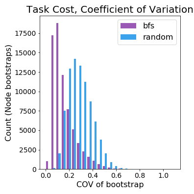
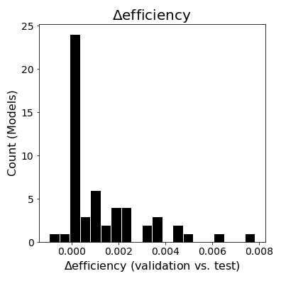
Figure 2. (Left) A distribution of the coefficient of variation ($\mu/\sigma$) over $b=20$ samples for a particular $C_{r}[i,k]$ set of classification instances, for Last.fm social. This estimates the median of $b=100$ with low error ($\leq 0.02$). (Right) The change in efficiency between validation and testing partitions: $\mathcal{E}(\mathcal{Q}_{r,test})-\mathcal{E}(\mathcal{Q}_{r,validation})$.

We now test the stability our choice of sampling parameters, over $b$, and across partitions. Figure 2 (Left) reports the coefficient of variation ($\mu/\sigma$) of task encoding costs for the $b$ classifiers in $C_{r}[i,k]$. These are smaller for the social-bfs model on Last.fm than for social-random. The median of these distributions at $b=20$ estimates the median at $b=100$ with low error ($\leq 0.02$) for a selection of models verified. Figure 2 (Right) reports the signed difference in efficiency between models on the test and validation partition. The models with $\Delta$efficiency $>0.004$ (or an increase of 250 bytes/correct) are all bfs on MovieLens, which may be a legitimate change in efficiency. This shows that our measurements are robust for estimating encoding cost at $k$, and efficiency is stable across partitions.

We test the stability of $\mathcal{E}(\mathcal{Q}_{r})$ and its correlation to correct predictions. Table 3 (Top) reports the Kendall’s tau rank order statistic measuring correlation between the ‘efficiency’ ranking of models. This further shows stability in the models between validation and testing partitions. Table 3 (Bottom) in contrast reports the $\tau$ between the ranked models according to efficiency, and according to correct predictions. Within the same partition, this rank correlation is lower than the efficiency rank correlation across partitions. This means that efficiency is quite stable in absolute error and relative ranking, and efficiency ranking is not merely a surrogate for ranking by correct prediction. Were this true, we would not need to encode the model. Nor are the ranks of these measures completely uncorrelated.

$\tau$, $\mathcal{E}(\mathcal{Q}_{r})$, Validation vs. Test
	Last.fm	MovieLens	BeerAdvocate
$\tau$	0.89	0.61	0.82
$p$-value	1e-8	5e-4	3e-6
$\tau$, $\mathcal{E}(\mathcal{Q}_{r})$ vs. $\operatorname*{correct}(\mathcal{C}_{r})$ (validation)
$\tau$	0.73	0.38	0.70
$p$-value	3e-6	0.03	7e-5

Table 3. (Top) The Kendall’s tau rank correlation coefficient between model efficiency of validation vs. test partitions. (Bottom) $\tau$ rank correlation between efficiency and correct predictions.

4.2. Efficiency features

Our definition of efficiency yields interpretable features which can characterize models and compare datasets. First, we compare the model and task encoding cost by calculating the ratio of model encoding cost to the total cost of encoding the model and collection of task models.

Second, recall that in the efficiency definition, we select the most efficient $\kappa_{i}$ per node $i$, with $\kappa_{i}\leq 150$ in our evaluation. This gives the model flexibility to search deeper in the query function for each $i$. Nodes with higher $\kappa_{i}$ are likely harder to classify because the task encoding is typically more expensive with more attribute-vector instances.

Figure 3 compares the ratio of model and total encoding costs (x-axis) vs. the mean over all $\kappa_{i}$ (y-axis). The models roughly order left-to-right on the x-axis according to Table 1.

All non-network models (activity-top, degree-top, cluster, random) are consistently inexpensive vs. their task models, but several also select a higher $\kappa_{i}$. In contrast, the degree-net and activity-net models are consistently costlier because they encode a fixed $m>\max(K)$ in order to sample at each value $k$. All ‘sorted’ models (network and non-network) tend to be most efficient at a lower $\kappa_{i}$. This may indicate these sorted nodes are more informative per instance, and each additional instance is more costly to incorporate into task models. Finally, bfs has high variance in encoding cost ratio depending on the reach of the underlying topology (Section 2.5.1).

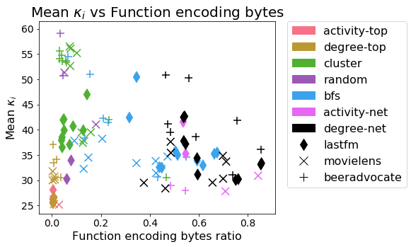
Figure 3. The mean over all $\kappa_{i}$: $\mathrm{mean}_{i}(\kappa_{i})$ vs. the ratio of model cost by the total encoding cost: $\operatorname*{bytes}(\mathcal{Q}_{r})/(\operatorname*{bytes}(\mathcal{Q}_{r})+\operatorname*{bytes}(\mathcal{C}_{r}))$. Colored by network query function, with markers by dataset.

4.3. Model selection

We now focus on selecting models from the efficiency ranking in the validation partition. We’ve already shown that there is high stability in the efficiency ranking between validation and testing partitions, but less correlation between correct predictions and efficiency (Table 3). Therefore, in this evaluation, we show we can recover the best model in test ($\mathcal{Q}_{best}$) with respect to correct predictions, using efficiency selection criteria.

Model Selection: $\mathcal{E}(\mathcal{Q}_{r})$, Evaluation: $\operatorname*{correct}(C_{r})$
$\mathcal{Q}_{select}$ (validation)	$\frac{\mathcal{E}(\mathcal{Q}_{select})}{\mathcal{E}(\mathcal{Q}_{best})}$	$\frac{\operatorname*{bytes}(\mathcal{Q}_{select})}{\operatorname*{bytes}(\mathcal{Q}_{best})}$	$\frac{\operatorname*{correct}(\mathcal{Q}_{select})}{\operatorname*{correct}(\mathcal{Q}_{best})}$
Last.fm, $\mathcal{Q}_{best}$: social-bfs
1. social-bfs	1.00	1.00	1.00
2. social-cluster	0.78	0.29	0.56
3. $\texttt{KNN}_{s}$-cluster	0.72	0.08	0.50
MovieLens, $\mathcal{Q}_{best}$: activity-top
1. activity-top	1.00	1.00	1.00
2. $\texttt{KNN}_{s}$-bfs	0.12	15.79	0.28
3. activity-net	0.20	130.14	0.91
BeerAdvocate, $\mathcal{Q}_{best}$: activity-net
1. activity-top	1.20	0.01	0.86
2. activity-net	1.00	1.00	1.00
3. $\texttt{KNN}_{s}$-cluster	0.22	0.09	0.20

Table 4. Model selection on ‘efficiency’ ranking in validation ($\mathcal{Q}_{select}$, Column 1) compared to the best model in test ranked by correct predictions ($\mathcal{Q}_{best}$), for efficiency, encoding cost, and correct prediction ratios (Columns 2,3,4).

The left-most column of Table 4 shows the three top-ranked models ($\mathcal{Q}_{select}$) by efficiency in validation. The ratios report the relative performance of the selected model (evaluated in test) for efficiency, total encoding size, and correct predictions.The second column–efficiency ratio–is not monotonically decreasing, because model ranking by efficiency may be different in test than validation (Table 3).

The selection by efficiency shows an intuitive trade-off between encoding cost and predictive performance. For Last.fm, the social-bfs model performs best, but the inexpensive social-cluster model is an alternative. This is consistent with previous results which show social-bfs is much more predictive than network adjacency, and of other underlying network models (Brugere et al., 2017a).

According to performance ratios, activity-net is extremely preferred in MovieLens and BeerAdvocate. This measures the extent that the most active users are also most informative in terms of efficiency in these two domains.

MovieLens correctly selects activity-top, and activity-net is an order of magnitude costlier while maintaining similar correct predictions. On BeerAdvocate, activity-net performs best on correct predictions, but activity-top is the better model since it preserves $0.86$ of correct predictions but is $0.01$ the encoding cost (it is first ranked by efficiency). This clearly shows why efficiency is preferred to favor parsimonious models.

Figure 4. Models ranked (x-axis) by efficiency (Left), total encoding cost $\operatorname*{bytes}(\mathcal{C}_{r})+\operatorname*{bytes}(\mathcal{Q}_{r})$ (Middle), and the number of correct predictions (Right).

Figure 4 reports models ranked by efficiency (Left) total encoding cost (Middle), and correct predictions (Right). The Last.fm ranking has more models because social are included. Ranking by correct predictions shows the extent that the top-ranked activity-net and activity-top models dominate the correct predictions on BeerAdvocate and MovieLens, which yields low ratios against $\mathcal{Q}_{best}$ in Table 4. Figure 4 (Middle) shows that each dataset grows similarly over our set of models, but that each has a different baseline of encoding cost. Last.fm is particularly costly; the median non-zero attributes per node (e.g. artists listened) is 578, or 7 times larger than MovieLens. These larger attribute vectors yield more expensive task models, requiring more bytes for the same correct predictions. These baselines also yield the same dataset ordering in efficiency. So, the worst model on MovieLens (random, 1084 bytes/correct) is more efficient than the best model on Last.fm (social-bfs, 1132 bytes/correct).

4.4. Model significance

In order to compare models with respect to a particular dataset, we measure the significance of each model relative to the efficiency over the complete set of models.

We compare the median difference of efficiency of $\mathcal{Q}_{r}$ to all other models against the median pairwise difference of all models excluding $\mathcal{Q}_{r}$, over the inter-quartile range (IQR) of pairwise difference. This measure is a non-parametric analogue to the $z$-score, where the median $\mathcal{Q}_{r}$ differences deviate from the pairwise expectation by at least a ‘$\lambda$’ factor of IQR.

Let $e_{i}=\mathcal{E}(\mathcal{Q}_{i})$, the efficiency value for an arbitrary network query function $\mathcal{Q}_{i}$, and $\lambda$ a significance level threshold, then for $i=1...|F|,j=1...|F|;i,j\neq r$:

(8) $$\mathrm{significance}(F,r,\lambda)=\\ \frac{\operatorname*{med}_{i}(|e_{r}-e_{i}|)-\operatorname*{med}_{i,j}(|e_{i}-e_{j}|)}{\operatorname*{iqr}_{i,j}(|e_{i}-e_{j}|)}\geq\lambda$$

This is a signed test favoring larger efficiency of $\mathcal{Q}_{r}$ than the expectation. The median estimates of the $e_{r}$ comparisons and pairwise comparisons are also robust to a small number of other significant models, and like the $z$-score, this test scales with the dispersion of the pairwise differences.

This test only assumes ‘significant’ models are an outlier class in all evaluated models $Q$. We propose a diverse set of possible representations; we use this diversity to treat consistency in the pairwise distribution as a robust null hypothesis: i.e. there is no appropriate model of the data within $Q$. Future work will more deeply focus on measuring this ‘diversity’, and determining the most robust set of models suitable for null modeling.

At $\lambda=1$ in validation, we find five significant models, corresponding to models reported in Table 4: social-bfs on Last.fm ($=1.30$), activity-top and activity-net on MovieLens ($=12.29,1.21$) and activity-top and activity-net on BeerAdvocate ($=7.64,~{}6.00$).

4.5. Model stability

For each of the significant models, we measure the impact of noise on its efficiency and significance. We apply node rewiring on the model we are testing, and leave all other models intact. For each neighbor of a node $i$, we re-wire $i$ to a new node at probability $p$. This is an out-degree preserving randomization, which is appropriate because outgoing edges determine the input for the task model on $i$. Sorting heuristics activity-net and degree-net are implemented as ad-hoc networks, where each node $i$ has directed edges to some $m$-sized subset of top-ranked nodes. For each top-ranked node adjacent to $i$, we re-map $i$ to a random node (possibly not in the top-ranked subset) with probability $p$. This again preserves the out-degree of $i$, and reduces the in-degree of top-ranked nodes.

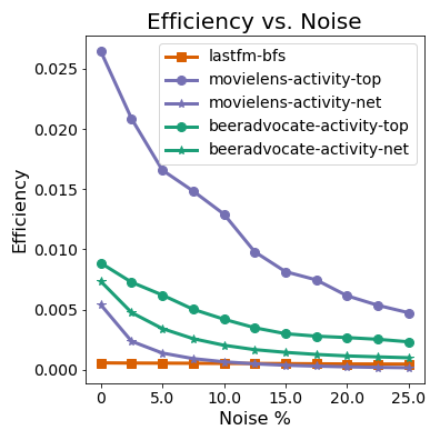
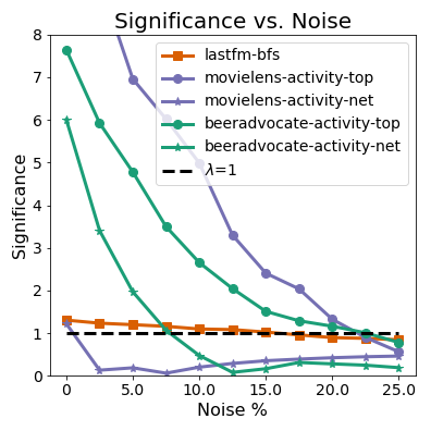
Figure 5. Varying level of noise for 5 ‘significant’ models (x-axis), reporting Efficiency (Left) and Significance (Right)

Figure 5 shows the effect of varying noise $p$ (x-axis), on the efficiency (Left), and significance (Right) of each significant model. activity-net on both MovieLens and BeerAdvocate quickly lose efficiency under even small noise, and are no longer significant for $\lambda=1$ at $p=0.025$, and $p=0.10$, respectively. activity-top is more robust, remaining significant to $p=0.225$.

activity-net is particularly sensitive to noise due to decreased performance in both encoding cost and correct predictions. At only $p=0.025$, activity-net on BeerAdvocate reduces in correct predictions by $15\%$ and increases in encoding cost by $31\%$. The encoding cost greatly increases because the cardinality of the set of unique numbers in the activity-net representation is small (bound by the size of the top-ranked sample). When random nodes are added in the representation, they are near-unique values, greatly increasing the set cardinality and reducing the compression ratio. activity-top shows a similar increase, but proportional to nodes rather than edges.

Finally, social-bfs is easily the most robust to noise. From a lower baseline, it remains significant to $p=0.15$. It loses only $35\%$ of its significance value at any noise level, while all other methods lose $>90\%$. This demonstrates that network models have robustness which might be desirable for further criteria in model selection. For example, our full methodology can be used to select on efficiency significance at some noise level $p$.

5. Conclusions and Future Work

In this paper, we have presented a minimum description length approach to perform model selection of networks. We have generalized networks as one particular representation of network query functions used to solve predictive tasks. This formulation allows comparing against arbitrary underlying representations and testing whether a network model is necessary in the first place. We propose a general efficiency measure for evaluating model selection for particular tasks on networks, and we show stability for node sampling and model ranking, as well as significance testing and sensitivity analysis for selected models. In total, this methodology is general and flexible enough to evaluate most networks inferred from attributed/labeled data, as well as networks given explicitly by the application of interest against alternative models.

There are several avenues for improving this work. First, exploiting model similarity and prioritizing novel models may more quickly discover significant models and estimate their value against the full null model enumeration. Furthermore, we aim to study which and how many models yield a robust baseline null distribution of efficiency measurements for model selection.

There are also extensions to this work. Currently, we learn node task models for each label instance. However, how many task models are needed on our network and can we re-use local models? Efficiency naturally measures the trade-off between eliminating task models vs. the loss in correct predictions. The aim is then task model-set summarization for maximum efficiency.

References

- (1)
- Brugere et al. (2016) I. Brugere, B. Gallagher, and T. Y. Berger-Wolf. 2016. Network Structure Inference, A Survey: Motivations, Methods, and Applications. ArXiv e-prints (Oct. 2016).
- Brugere et al. (2017a) Ivan Brugere, Chris Kanich, and Tanya Berger-Wolf. 2017a. Evaluating Social Networks Using Task-Focused Network Inference. In Proceedings of the 13th International Workshop on Mining and Learning with Graphs (MLG).
- Brugere et al. (2017b) Ivan Brugere, Chris Kanich, and Tanya Y. Berger-Wolf. 2017b. Network Model Selection for Task-Focused Attributed Network Inference. In 2017 IEEE International Conference on Data Mining Workshop (ICDMW).
- Caceres and Berger-Wolf (2013) Rajmonda Sulo Caceres and Tanya Berger-Wolf. 2013. Temporal Scale of Dynamic Networks. 65–94.
- Caceres et al. (2016) R. S. Caceres, L. Weiner, M. C. Schmidt, B. A. Miller, and W. M. Campbell. 2016. Model Selection Framework for Graph-based data. ArXiv e-prints (Sept. 2016).
- Efron and Tibshirani (1993) B Efron and R J Tibshirani. 1993. An Introduction to the Bootstrap. Chapman & Hall.
- Ferlez et al. (2008) J. Ferlez, C. Faloutsos, J. Leskovec, D. Mladenic, and M. Grobelnik. 2008. Monitoring Network Evolution using MDL. In 2008 IEEE 24th International Conference on Data Engineering. 1328–1330.
- Hamilton et al. (2017) W. L. Hamilton, R. Ying, and J. Leskovec. 2017. Representation Learning on Graphs: Methods and Applications. ArXiv e-prints (Sept. 2017).
- Hansen and Yu (2001) Mark H Hansen and Bin Yu. 2001. Model Selection and the Principle of Minimum Description Length. J. Amer. Statist. Assoc. 96, 454 (2001), 746–774.
- Harper and Konstan (2015) F Maxwell Harper and Joseph A Konstan. 2015. The MovieLens Datasets: History and Context. ACM Trans. Interact. Intell. Syst. 5, 4 (dec 2015), 19:1—-19:19.
- Hasan and Zaki (2011) Mohammad Al Hasan and Mohammed J. Zaki. 2011. A Survey of Link Prediction in Social Networks. In Social Network Data Analytics SE - 9. 243–275.
- Hu et al. (2011) Bing Hu, Thanawin Rakthanmanon, Yuan Hao, Scott Evans, Stefano Lonardi, and Eamonn Keogh. 2011. Discovering the Intrinsic Cardinality and Dimensionality of Time Series Using MDL. In Proceedings of the 2011 IEEE 11th International Conference on Data Mining. 1086–1091.
- Kim and Leskovec (2012) Myunghwan Kim and Jure Leskovec. 2012. Multiplicative Attribute Graph Model of Real-World Networks. Internet Mathematics 8, 1-2 (Mar. 2012), 113–160.
- Kolaczyk (2009) Eric D. Kolaczyk. 2009. Network Topology Inference. In Statistical Analysis of Network Data SE - 7. Springer New York, 1–48.
- Koutra et al. (2014) Danai Koutra, U Kang, Jilles Vreeken, and Christos Faloutsos. 2014. VOG: Summarizing and Understanding Large Graphs. In Proceedings of the 2014 SIAM International Conference on Data Mining. 91–99.
- Liben-Nowell and Kleinberg (2007) David Liben-Nowell and Jon Kleinberg. 2007. The link-prediction problem for social networks. Journal of the American Society for Information Science and Technology 58, 7 (May 2007), 1019–1031.
- McAuley et al. (2012) Julian McAuley, Jure Leskovec, and Dan Jurafsky. 2012. Learning Attitudes and Attributes from Multi-aspect Reviews. In Proceedings of the 2012 IEEE International Conference on Data Mining. 1020–1025.
- Mehta et al. (1996) Manish Mehta, Rakesh Agrawal, and Jorma Rissanen. 1996. SLIQ: A fast scalable classifier for data mining. 18–32.
- Namata et al. (2015) Galileo Mark Namata, Ben London, and Lise Getoor. 2015. Collective Graph Identification. ACM Transactions on Knowledge Discovery from Data.
- Pfeiffer III et al. (2014) Joseph J Pfeiffer III, Sebastian Moreno, Timothy La Fond, Jennifer Neville, and Brian Gallagher. 2014. Attributed Graph Models: Modeling Network Structure with Correlated Attributes. In Proceedings of the 23rd International Conference on World Wide Web. ACM, 831–842.
- Rissanen (2004) Jorma Rissanen. 2004. Minimum Description Length Principle. John Wiley & Sons, Inc.
- Sun et al. (2007) Jimeng Sun, Christos Faloutsos, Spiros Papadimitriou, and Philip S Yu. 2007. GraphScope: parameter-free mining of large time-evolving graphs. In Proceedings of the 13th ACM SIGKDD international conference on Knowledge discovery and data mining (KDD ’07). ACM, 687–696.
- Takahashi et al. (2012) Daniel Yasumasa Takahashi, João Ricardo Sato, Carlos Eduardo Ferreira, and André Fujita. 2012. Discriminating Different Classes of Biological Networks by Analyzing the Graphs Spectra Distribution. PLOS ONE 7, 12 (12 2012), 1–12.
- Vishwanathan et al. (2010) S. V. N. Vishwanathan, Nicol N. Schraudolph, Risi Kondor, and Karsten M. Borgwardt. 2010. Graph Kernels. J. Mach. Learn. Res. 11 (Aug. 2010), 1201–1242.
- Zhao et al. (2006) Wentao Zhao, Erchin Serpedin, and Edward R. Dougherty. 2006. Inferring gene regulatory networks from time series data using the minimum description length principle. Bioinformatics 22, 17 (2006), 2129–2135.