Hyper-reduction over nonlinear manifolds for large nonlinear mechanical systems

Abstract

Common trends in model reduction of large nonlinear finite-element-discretized systems involve Galerkin projection of the governing equations onto a low-dimensional linear subspace. Though this reduces the number of unknowns in the system, the computational cost for obtaining the reduced solution could still be high due to the prohibitive computational costs involved in the evaluation of nonlinear terms. Hyper-reduction methods are then used for fast approximation of these nonlinear terms. In the finite-element context, the energy conserving sampling and weighing (ECSW) method has emerged as an effective tool for hyper-reduction of Galerkin-projection-based reduced-order models (ROM).

More recent trends in model reduction involve the use of nonlinear manifolds, which involves projection onto the tangent space of the manifold. While there are many methods to identify such nonlinear manifolds, hyper-reduction techniques to accelerate computation in such ROMs are rare. In this work, we propose an extension to ECSW to allow for hyper-reduction using nonlinear mappings, while retaining its desirable stability and structure-preserving properties. As a proof of concept, the proposed hyper-reduction technique is demonstrated over models of a flat plate and a realistic wing structure, whose dynamics have been shown to evolve over a nonlinear (quadratic) manifold. An online speed-up of over one thousand times relative to the full system has been obtained for the wing structure using the proposed method, which is higher than its linear counterpart using the ECSW.
Keywords: EECSW; nonlinear manifolds; ECSW; hyper-reduction; model order reduction; structure-preserving; nonlinear dynamics; Galerkin projection

1 Introduction

Model reduction and hyper-reduction

In spite of the ever increasing computational power and digital storage capabilities, reduced-order models (ROM) of Finite Element (FE) discretized systems are a must when complex simulations are needed to support design and optimization activities. Current state-of-the-art ROM techniques are based on a reduced basis approach, i.e., the solution is sought on a linear, low-dimensional subspace spanned by a few, carefully selected modes. The resulting residual is then projected onto the same or a different subspace of the same dimension to obtain a well-posed reduced system. When the original system of equations–often referred to as high-fidelity model (HFM)–features symmetric operators, the residual is projected on the same basis used for the approximation of the solution. This procedure is known as the Bubnov-Galerkin projection. The dimensionality reduction is guaranteed by the limited number of reduction variables as compared to the number of degrees of freedom in the HFM.

Assuming granted accuracy, projection-based ROMs are not able to deliver significant speedups, when applied to nonlinear systems. This is due to the fact that the computation of the reduced nonlinear terms at each solver iteration scales with the dimensionality of the HFM rather than with that of the reduction subspace. In the case of polynomial nonlinearities, one might consider pre-computing the reduced nonlinear term [19, 18, 16], leading to higher-order tensors. Typically, FE models may also contain rotational DOFs, where the associated nonlinearity cannot be pre-computed and stored in the form of tensors. Furthermore, for high polynomial degrees, the computations with higher-order tensors can become intractable, even more so than the HFM simulations [16]. For such cases, in the most general setting, the above-mentioned scalability issue is successfully alleviated by a range of hyper-reduction techniques, which aim at significantly reducing the cost of reduced nonlinear term evaluation by computing them only at few, selected elements or nodes of the FE models, and cheaply approximating the missing information.

The Gappy POD method [20], first introduced for image reconstruction and later applied in dynamical systems [22, 23], was one of the first instances of hyper-reduction. However, as observed by Farhat et al. [5], the term hyper-reduction was introduced much later in [15], where a selection of the integration point in a FE model is performed in an a priori manner. The empirical interpolation method (EIM) [4] approximates a non-affine function using a set of basis functions over a continuous, bounded domain, and hence finds applications for reduced basis representations of parameterized partial differential equations (PDEs). The discrete empirical interpolation method (DEIM) [1] achieves this on a discrete state space. For FE applications, the unassembled DEIM or UDEIM [2] was shown to be more efficient, where the unassembled element-level nonlinear force vector is used in the DEIM algorithm to return a small set of elements (instead of nodes) over which the nonlinearity is evaluated. For conservative/port-Hamiltonian systems, however, the DEIM (or UDEIM) leads to a loss of numerical stability during time integration. Though a symmetrized version of DEIM has been proposed recently [3] to avoid this issue, its potential for FE-based applications remains unexplored. To this end, the energy-conserving sampling and weighting (ECSW) hyper-reduction method [5] is remarkable. The ECSW method directly approximates the reduced nonlinear term and is particularly well-suited for FE-based structural dynamics applications, as it preserves the symmetry of the operators involves and leads to numerical stability.

The main idea of ECSW is simple yet powerful: only few elements are interrogated to compute the nonlinear forces, and weights (obtained using training) are attached to them to match the virtual work done by their full counterparts onto virtual displacements given by the linear reduction basis vectors. Albeit being efficient and relevant for FE-based mechanical systems, the ECSW hyper-reduction method is proposed in the context of linear mappings from the space of reduced variables. To the best of the authors’ knowledge, this is a common feature of all other hyper-reduction techniques in the literature, as well.

Nonlinear manifolds in model reduction

It is quite natural, however, for the dynamics of general nonlinear systems to evolve on inherently nonlinear manifolds, and not over linear subspaces (cf. [21] for a discussion). Often, a nonlinear manifold relevant for system dynamics may not be embeddable in a low-dimensional linear subspace. It is then easy to see that the linear-mapping-based ROM would either fail to capture the system response, or require frequent basis-updates (online) to account for the nonlinearity of the manifold, making the reduction process cumbersome and possibly redundant due to high computational costs in setting up such a ROM. Many methods allow for model reduction using attracting nonlinear manifolds in nonlinear dynamical systems – from a theoretical, as well as a data-driven, statistical perspective.

The approximate inertial manifold (AIM) provides an approximation of the solution of a PDE over sufficiently long time scales, using the theory of inertial manifolds. This is done by enslaving the amplitudes of fast modes in the system as a smooth graph over the amplitudes of a few selected modes while assuming that the corresponding inertial forces are not excited (see [26, 6], for instance). The so called static condensation approach (cf. [18]) achieves the same objective without the projection of the governing equations on to eigenfunctions. This is usually done for systems exhibiting a dichotomy of unknowns, such as the axial (in-plane) and transverse (out-of-plane) unknowns in a beam or a plate. From the perspective of nonlinear dynamics, a good overview of nonlinear model reduction techniques can be found in [25] and the references therein.

Over the past decade or so, the use of nonlinear manifolds in model reduction has received a significant boost by many data-driven techniques, broadly referred to as nonlinear dimensionality reduction (NLDR) or manifold learning, see [14], for instance. These techniques aim at constructing low dimensional manifolds from high-dimensional data snapshots. In a ROM perspective, these snapshots may be extracted from simulations of the underlying HFM, and the chosen NLDR is deemed to provide a nonlinear mapping with the required smoothness [9]. In essence, these methods provide a nonlinear generalization of the Proper Orthogonal Decomposition (POD), a well-known technique which delivers an optimal linear subspace for the dimensionality reduction.

The use of nonlinear manifolds in model reduction is expected to not only further reduce the dimensionality of the ROM in contrast to its linear mapping counterpart, but also shed light on the underlying system behaviour. This is especially true for the case of thin walled structures, which exhibit a time scale separation between slow, out-of-plane; and fast, in-plane dynamics. The fast dynamics in such systems can often be enslaved statically to the slow one, in a nonlinear fashion [8]. Recent efforts [11, 12] have shown that the geometrically nonlinear dynamics of structures, characterized by bending-stretching coupling (as for instance, thin walled components) can be effectively captured using a quadratic manifold (QM), constructed using model properties rather then HFM snapshots.

Our contribution

The nonlinear-manifold-based ROMs are usually obtained by projecting the HFM on the tangent space of the manifold, in a virtual work sense. This generates configuration-dependent inertial terms for the ROM in addition to the already existing projected nonlinear terms. For general nonlinear systems, the evaluation and projection of the nonlinearity remains a bottleneck for computations, much like the linear mapping counterpart. As discussed above, the state-of-the-art hyper-reduction techniques allow for fast approximation of the (projected) nonlinearity in the case of linear-mapping-based ROMs. This functionality, however, has been missing in the context of nonlinear-manifold-based ROMs.

In this contribution, we generalize the application of the ECSW hyper-reduction method to nonlinear-manifold-based ROMs. This work is essentially inspired from the ideas in the seminal work of Farhat et al. [5, 7], where ECSW method was introduced in the context of linear mappings. Following similar lines as in [7], we further show that our extension of the ECSW (hereafter referred to as extended ECSW: EECSW, for comparison purposes) preserves the Lagrangian structure associated with the Hamilton’s principle. A natural consequence of this property is numerical stability during time integration, as shown in [7]. The proposed method is tested, first on an academically simple example, and then on a realistic model of a wing using the recently proposed QM for reduction. Our numerical results indicate that better speed ups can be achieved, as compared to the ones obtained with a linear POD subspace reduction equipped with ECSW. Interestingly, EECSW selects fewer elements for the hyper-reduction as compared to its linear counterpart, and more than compensates the extra computational costs associated to the configuration dependent inertial terms, which are not present in the case of linear subspace reduction.

This paper is organized as follows. The concept of projection-based ROM on nonlinear mappings is briefly reviewed in Section 2. The extension of ECSW for nonlinear mappings is the tackled in Section 3, where also the preservation of the Lagrangian structure of the thus-obtained ROM is shown. Numerical results showing the effectiveness of the method are reported in Section 4, and finally, the conclusions are given in Section 5.

2 Model reduction using nonlinear mappings

The partial differential equations (PDEs) for momentum balance in a structural continuum are usually discretized along the spatial dimensions using finite elements to obtain a system of second-order ordinary differential equations (ODEs). Along with the initial conditions for generalized displacements and velocities, these ODEs govern the response of the underlying structure. More specifically, this response can be described by the solution to an initial value problem (IVP) of the following form:

$$\mathbf{\begin{gathered}\mathbf{M}\ddot{\mathbf{u}}(t)+\mathbf{C}\dot{\mathbf{u}}(t)-\mathbf{f}(\mathbf{u}(t))=\mathbf{f}^{ext}(t)\,,\\ \mathbf{u}(t_{0})=\mathbf{u}_{0},\,\dot{\mathbf{u}}(t_{0})=\mathbf{v}_{0},\end{gathered}}$$ (3)

where the solution $\mathbf{u}(t)\in\mathbb{R}^{n}$ is a high-dimensional generalized displacement vector, $\mathbf{M}\in\mathbb{R}^{n\times n}$ is the mass matrix; $\mathbf{C}\in\mathbb{R}^{n\times n}$ is the damping matrix; $\mathbf{f}:\mathbb{R}^{n}\mapsto\mathbb{R}^{n}$ gives the nonlinear elastic internal force as a function of of the displacement $\mathbf{u}$ of the structure; and $\mathbf{f}^{ext}(t)\in\mathbb{R}^{n}$ is the time dependent external load vector. The system (3), referred to as the high-fidelity model (HFM), exhibits prohibitive computational costs for large values of the dimension $n$ of the system. The classical notion of model reduction aims to reduce this dimensionality by introducing a linear mapping onto a suitable low-dimensional invariant subspace. However, as discussed in the Introduction, more recent advances in model reduction allow for the detection of system dynamics evolving over nonlinear manifolds. The idea of a projection-based reduced-order model using nonlinear mappings was presented in [11], using a nonlinear mapping such as

$$\mathbf{u}(t)\approx\boldsymbol{\Gamma}(\mathbf{q}(t)),$$ (4)

where $\boldsymbol{\Gamma}:\mathbb{R}^{m}\mapsto\mathbb{R}^{n}$ is the nonlinear mapping function. In general the mapping (4), when substituted into the governing equations (3), results in a non-zero residual $\mathbf{r}$ as

$$\mathbf{M}\ddot{\boldsymbol{\Gamma}}\left(\mathbf{q}(t)\right)+\mathbf{C}\dot{\boldsymbol{\Gamma}}\left(\mathbf{q}(t)\right)-\mathbf{f}\left(\boldsymbol{\Gamma}\left(\mathbf{q}(t)\right)\right)-\mathbf{f}^{ext}(t)=\mathbf{\mathbf{r}}.$$

The virtual work principle for a kinematically admissible displacement, $\delta\mathbf{u}=\frac{\partial\boldsymbol{\Gamma}(\mathbf{q})}{\partial\mathbf{q}}\delta\mathbf{q}$, over the nonlinear manifold leads to

$$\mathbf{\mathbf{r}}\cdot\delta\mathbf{u}=0$$

$$\implies\left[\mathbf{M}\ddot{\boldsymbol{\Gamma}}\left(\mathbf{q}(t)\right)+\mathbf{C}\dot{\boldsymbol{\Gamma}}\left(\mathbf{q}(t)\right)-\mathbf{f}\left(\boldsymbol{\Gamma}\left(\mathbf{q}(t)\right)\right)\right]\cdot\delta\mathbf{u}=\mathbf{f}^{ext}(t)\cdot\delta\mathbf{u}\,.$$

Physically, this means that the residual force is orthogonal to the tangent space of the manifold. This gives the corresponding reduced-order model as

$$\mathbf{P}_{\boldsymbol{\Gamma}}^{T}(\mathbf{q})\left[\mathbf{M}\ddot{\boldsymbol{\Gamma}}\left(\mathbf{q}(t)\right)+\mathbf{C}\dot{\boldsymbol{\Gamma}}\left(\mathbf{q}(t)\right)-\mathbf{f}\left(\boldsymbol{\Gamma}\left(\mathbf{q}(t)\right)\right)\right]=\mathbf{P}_{\boldsymbol{\Gamma}}^{T}(\mathbf{q})\mathbf{f}^{ext}(t),$$ (5)

where $\mathbf{P}_{\boldsymbol{\Gamma}}(\mathbf{q}):=\frac{\partial\boldsymbol{\Gamma}(\mathbf{q})}{\partial\mathbf{q}}\in\mathbb{R}^{n\times m}$ represents the tangent space of the nonlinear manifold in which the system dynamics is expected to evolve. Hereafter, we shall omit the dependence of $\mathbf{P}_{\boldsymbol{\Gamma}}$ on $\mathbf{q}$. The acceleration and velocity vectors over the manifold can be evaluated using the chain rule as

$$\dot{\boldsymbol{\Gamma}}\left(\mathbf{q}(t)\right) =\frac{d}{dt}\boldsymbol{\Gamma}\left(\mathbf{q}(t)\right)=\frac{\partial\boldsymbol{\Gamma}(\mathbf{q})}{\partial\mathbf{q}}\cdot\dot{\mathbf{q}},$$

$$\ddot{\boldsymbol{\Gamma}}\left(\mathbf{q}(t)\right) =\frac{d}{dt}\dot{\boldsymbol{\Gamma}}\left(\mathbf{q}(t)\right)=\frac{\partial\boldsymbol{\Gamma}(\mathbf{q})}{\partial\mathbf{q}}\cdot\ddot{\mathbf{q}}+\left[\frac{\partial^{2}\boldsymbol{\Gamma}(\mathbf{q})}{\partial\mathbf{q}\partial\mathbf{q}}\cdot\dot{\mathbf{q}}\right]\cdot\dot{\mathbf{q}}\,.$$

Using the above relations, (5) can also be expressed as

$$\mathbf{M}_{r}(\mathbf{q})\,\ddot{\mathbf{q}}+\mathbf{C}_{r}(\mathbf{q},\dot{\mathbf{q}})\,\dot{\mathbf{q}}-\mathbf{f}_{r}(\mathbf{q})=\mathbf{P}_{\boldsymbol{\Gamma}}^{T}\mathbf{f}^{ext}(t)\,,$$ (6)

where $\mathbf{M}_{r}(\mathbf{q})=\mathbf{P}_{\boldsymbol{\Gamma}}^{T}\mathbf{M}\mathbf{P}_{\boldsymbol{\Gamma}}$, $\mathbf{C}_{r}(\mathbf{q},\dot{\mathbf{q}})=\mathbf{P}_{\boldsymbol{\Gamma}}^{T}\mathbf{C}\mathbf{P}_{\boldsymbol{\Gamma}}+\mathbf{P}_{\boldsymbol{\Gamma}}^{T}\mathbf{M}\left(\frac{\partial^{2}\boldsymbol{\Gamma}(\mathbf{q})}{\partial\mathbf{q}\partial\mathbf{q}}\cdot\dot{\mathbf{q}}\right)$ and $\mathbf{f}_{r}(\mathbf{q})=\mathbf{P}_{\boldsymbol{\Gamma}}^{T}\mathbf{f}(\boldsymbol{\Gamma}(\mathbf{q}))$.

Note that for $\boldsymbol{\Gamma}$ being a linear function, such that $\boldsymbol{\Gamma}(\mathbf{q})=\mathbf{V}\mathbf{q}$ (for some $\mathbf{V}\in\mathbb{R}^{n\times m}$ spanning a suitable low dimensional subspace), the ROM in (5) reduces to the familiar Galerkin-projection-based ROMs as

$$\mathbf{V}^{T}\mathbf{M}\mathbf{V}\ddot{\mathbf{q}}(t)+\mathbf{V}^{T}\mathbf{C}\mathbf{V}\dot{\mathbf{q}}(t)-\mathbf{V}^{T}\mathbf{f}(\mathbf{Vq}(t))=\mathbf{V}^{T}\mathbf{f}^{ext}(t).$$ (7)

During time integration–usually referred to as the online phase–of (7), the computational cost associated to the evaluation of the linear terms in (7) scales only with the number of reduced variables $m$, since the corresponding reduced operators can be pre-computed offline. However, this is not the case for the computation of the reduced nonlinear term $\mathbf{V}^{T}\mathbf{f}(\mathbf{Vq}(t))$. Specifically, for FE-based applications, this evaluation is usually carried out online, in the following manner:

$$\hat{\mathbf{f}}(\mathbf{q}):=\mathbf{V}^{T}\mathbf{f}(\mathbf{Vq})=\sum_{e=1}^{n_{e}}\mathbf{V}_{e}^{T}\mathbf{f}_{e}(\mathbf{V}_{e}\mathbf{q}),$$ (8)

where $\mathbf{f}_{e}(\mathbf{u_{e}})\in\mathbb{R}^{N_{e}}$ is the contribution of the element $e$ towards the vector $\mathbf{f}(\mathbf{u})$ ($N_{e}$ being the number of DOFs for the element $e$), $\mathbf{V}_{e}$ is the restriction of $\mathbf{V}$ to the rows indexed by the DOFs corresponding to $e$, and $n_{e}$ is the total number of elements in the structure. It is then easy to see from (8), that the cost associated to the computation of the reduced nonlinear force $\hat{\mathbf{f}}(\mathbf{q})$ scales linearly with the total number of elements $n_{e}$ in the structure, which is potentially high for large systems. Thus, despite the reduction in dimensionality achieved in (7), the evaluation of the reduced nonlinear term $\hat{\mathbf{f}}(\mathbf{q})$ emerges as a new bottleneck for the fast prediction of system response using the ROM (7). Similar conclusions regarding computational bottlenecks hold for the nonlinear-reduction-based ROM (5), as well.

3 Hyper-reduction and Extended ECSW

Hyper-reduction techniques help mitigate the above-stated high computational costs by approximation of the reduced-nonlinear term in a computationally affordable manner. As discussed in the Introduction, the ECSW [5] is a remarkable method for hyper-reduction of linear-mapping-based ROMs, such as that in (7). After briefly summarizing ECSW, we propose here a natural extension to ECSW, which facilitates hyper-reduction of nonlinear-manifold-based ROM, such as in (5). Much like the ECSW, we further show in Section 3.2 that the proposed EECSW preserves the Lagrangian structure associated to the underlying mechanical system and, hence, leads to numerical stablity in time integration.

In ECSW [5], the computationally expensive reduced nonlinear forces such as $\hat{\mathbf{f}}(\mathbf{q})$ (cf. (8)) in the Galerkin-projection-based ROMs, e.g., (7) is approximated as

$$\text{(ECSW)}\quad\hat{\mathbf{f}}(\mathbf{q})\approx\tilde{\mathbf{f}}(\mathbf{q}):=\sum_{e\in E}\xi_{e}\mathbf{V}_{e}^{T}\mathbf{f}_{e}(\mathbf{V}_{e}\mathbf{q}),$$ (9)

where $\xi_{e}\in\mathbb{R}^{+}$ is a positive weight given to every element $e\in E$. Clearly, the evaluation of $\tilde{\mathbf{f}}(\mathbf{q})$ in (9) comes at a fraction of the computational cost associated to (8), for $|E|\ll n_{e}$. This is made possible with weights which are chosen using training to ensure a good approximation of the original sum over all $n_{e}$ elements, while keeping the element sample small using sparse algorithms in literature. The element-set $E$ is sometimes referred to as the reduced mesh due to its low cardinality relative to the total number of elements $n_{e}$. Farhat et al. [7] further show that hyper-reduction done in this manner preserves Lagrangian structure of the linear Galerkin-projection-based ROMs.

We observe that analogous to (8), the projected nonlinear force (possibly a combination of inertial, damping or elastic forces) in the nonlinear ROM (5) can be expressed as a summation of the element-level contributions as

$$\boldsymbol{\mathfrak{h}}_{r}(\mathbf{q},\dot{\mathbf{q}},\ddot{\mathbf{q}}):=\mathbf{P}_{\boldsymbol{\Gamma}}^{T}\boldsymbol{\mathfrak{h}}\left(\boldsymbol{\Gamma}(\mathbf{q}),\dot{\boldsymbol{\Gamma}}\left(\mathbf{q}\right),\ddot{\boldsymbol{\Gamma}}\left(\mathbf{q}\right)\right)=\sum_{e=1}^{n_{e}}\left(\mathbf{P}_{\boldsymbol{\Gamma}}(\mathbf{q})\right)_{e}^{T}\boldsymbol{\mathfrak{h}}_{e}\left(\boldsymbol{\Gamma}_{e}(\mathbf{q}),\dot{\boldsymbol{\Gamma}}_{e}\left(\mathbf{q}\right),\ddot{\boldsymbol{\Gamma}}_{e}\left(\mathbf{q}\right)\right),$$ (10)

where $\boldsymbol{\mathfrak{h}}_{r}\left(\mathbf{q},\dot{\mathbf{q}},\ddot{\mathbf{q}}\right)$ is the part of the ROM (5) which is potentially unaffordable to compute (cost scales with $n$ or $n_{e}$), $\boldsymbol{\mathfrak{h}}$ is its full counterpart, with the $\boldsymbol{\mathfrak{h}}_{e}$ having the usual meaning for the element-level contribution from the element $e$. Just like in ECSW, the summation in (10) may be approximated as

$$\text{(EECSW)}\quad\boldsymbol{\mathfrak{h}}_{r}(\mathbf{q},\dot{\mathbf{q}},\ddot{\mathbf{q}})\approx\tilde{\boldsymbol{\mathfrak{h}}}_{r}(\mathbf{q},\dot{\mathbf{q}},\ddot{\mathbf{q}})=\sum_{e\in E}\xi_{e}\left(\mathbf{P}_{\boldsymbol{\Gamma}}(\mathbf{q})\right)_{e}^{T}\boldsymbol{\mathfrak{h}}_{e}\left(\boldsymbol{\Gamma}_{e}(\mathbf{q}),\dot{\boldsymbol{\Gamma}}_{e}\left(\mathbf{q}\right),\ddot{\boldsymbol{\Gamma}}_{e}\left(\mathbf{q}\right)\right),$$ (11)

where $\xi_{e}\in\mathbb{R}^{+}$ is again a positive weight given to every element $e$ in the reduced mesh $E$. The element sampling and weighing are discussed in Section 3.1

One easily observable distinction of EECSW from its linear mapping counterpart is that in ECSW, it is possible to precompute the reduced linear operators in the hyper-reduced model, such as the reduced mass, damping and stiffness matrices $\mathbf{V}^{T}\mathbf{M}\mathbf{V}$, $\mathbf{V}^{T}\mathbf{C}\mathbf{V}$ and $\mathbf{V}^{T}\mathbf{K}\mathbf{V}$, respectively. Due to the nonlinear mapping and projection on the tangent space, we see that EECSW doesn’t feature reduced-linear operators, even for the linear mass, stiffness and damping matrices in the HFM. Thus, in principle, one could include all the terms on the left hand of (5) in $\boldsymbol{\mathfrak{h}}_{r}$, i.e.,

$$\boldsymbol{\mathfrak{h}}_{r}(\mathbf{q},\dot{\mathbf{q}},\ddot{\mathbf{q}})=\mathbf{P}_{\boldsymbol{\Gamma}}^{T}\left[\mathbf{M}\ddot{\boldsymbol{\Gamma}}\left(\mathbf{q}(t)\right)+\mathbf{C}\dot{\boldsymbol{\Gamma}}\left(\mathbf{q}(t)\right)-\mathbf{f}\left(\boldsymbol{\Gamma}\left(\mathbf{q}(t)\right)\right)\right].$$

It is easy to see that this idea is a straight-forward generalization of ECSW to nonlinear-manifold-based ROMs with projection to the tangent space, as given in (5). Indeed, for $\boldsymbol{\Gamma}(\mathbf{q})=\mathbf{V}\mathbf{q}$, hyper-reduction of ROM (7) results in the same approximation of the projected internal force as in (8).

3.1 Element sampling and weight selection

The elements and weights are determined to approximate virtual work over chosen training sets which generally come from full solution run(s). We assume that $\left\{\mathbf{u}^{(i)},\dot{\mathbf{u}}^{(i)},\ddot{\mathbf{u}}^{(i)}\right\},\,i\in\{1,\dots,n_{t}\}$ represents a set of available training vectors. If the solution to the HFM, indeed, evolves over a nonlinear manifold as given by (4), then we must be able to find reduced unknowns $\left\{\mathbf{q}^{(i)},\dot{\mathbf{q}}^{(i)},\ddot{\mathbf{q}}^{(i)}\right\}$ such that

$$\left.\begin{aligned} \mathbf{u}^{(i)}&=\boldsymbol{\Gamma}\left(\mathbf{q}^{(i)}\right)\\ \dot{\mathbf{u}}^{(i)}&=\mathbf{P}_{\boldsymbol{\Gamma}}\left(\mathbf{q}^{(i)}\right)\dot{\mathbf{q}}^{(i)}\\ \ddot{\mathbf{u}}^{(i)}&=\mathbf{P}_{\boldsymbol{\Gamma}}^{T}\left(\mathbf{q}^{(i)}\right)\ddot{\mathbf{q}}^{(i)}+\left[\left.\frac{\partial^{2}\boldsymbol{\Gamma}(\mathbf{q})}{\partial\mathbf{q}\partial\mathbf{q}}\right|_{\mathbf{q}=\mathbf{q}^{(i)}}\cdot\dot{\mathbf{q}}^{(i)}\right]\cdot\dot{\mathbf{q}}^{(i)}\end{aligned}\right\}\quad\forall i\in\{1,\dots,n_{t}\}\,.$$ (12)

As will be clear later in this section, the optimal elements and weights corresponding to a reduced mesh needs the set of reduced vectors $\left\{\mathbf{q}^{(i)},\dot{\mathbf{q}}^{(i)},\ddot{\mathbf{q}}^{(i)}\right\}$ during the training stage. In case these are available from a previous ROM simulation, these would be directly useful. Furthermore, if the nonlinear manifold is obtained from solution snapshots using manifold-learning procedures such as the local maximum entropy approximants, as done in, e.g, [9], then the reduced vectors would be directly available from the manifold-learning procedure. However, if the manifold is obtained from simulation-free approaches (cf. [11, 12]), then a nonlinear system of algebraic equations (12) can be solved for the reduced training vectors $\mathbf{q}^{(i)},\dot{\mathbf{q}}^{(i)},\text{and }\ddot{\mathbf{q}}^{(i)}$. This system is under-constrained ($m\ll n$) and , hence, the sought $\mathbf{q}^{(i)}$ can be obtained from the solution to a nonlinear least-squares procedures, e.g., the gradient descent method, the Gauss-Newton methods, the Levenberg-Marquardt method (which is also employed in the standard LSQNONLIN routine in MATLAB); we refer the reader to [13] for a review of standard methods for nonlinear least squares problems.

Geometrically, the first equation in the system (12) gives the location of the data point on the manifold, whereas as the second and the third equations give the trajectory information (tangent and curvature along the trajectory). Thus, the reduced coordinates of the point on the manifold can be identified independent of the velocity and acceleration information by solving the equation

$$\mathbf{q}^{(i)}=\arg\min_{\mathbf{q}\in\mathbb{R}^{m}}\left\|\boldsymbol{\Gamma}\left(\mathbf{q}\right)-\mathbf{u}^{(i)}\right\|_{2}^{2}.$$ (13)

Though the nonlinear least squares problem (13) would add to the offline costs, note that this procedure is embarassingly parallelizable for each training snapshot. Once the reduced coordinates $\mathbf{q}^{(i)}$ are obtained on the manifold, the second equation in (12) can be solved in a least squares sense for $\dot{\mathbf{q}}^{(i)}$ as

$$\dot{\mathbf{q}}^{(i)}=\left[\mathbf{P}_{\boldsymbol{\Gamma}}^{T}\left(\mathbf{q}^{(i)}\right)\mathbf{P}_{\boldsymbol{\Gamma}}\left(\mathbf{q}^{(i)}\right)\right]^{-1}\mathbf{P}_{\boldsymbol{\Gamma}}^{T}\left(\mathbf{q}^{(i)}\right)\dot{\mathbf{u}}^{(i)}.$$ (14)

Finally, we can obtain the corresponding reduced accelerations as

$$\ddot{\mathbf{q}}^{(i)}=\left[\mathbf{P}_{\boldsymbol{\Gamma}}^{T}\left(\mathbf{q}^{(i)}\right)\mathbf{P}_{\boldsymbol{\Gamma}}\left(\mathbf{q}^{(i)}\right)\right]^{-1}\mathbf{P}_{\boldsymbol{\Gamma}}^{T}\left(\mathbf{q}^{(i)}\right)\left(\ddot{\mathbf{u}}^{(i)}-\left[\left.\frac{\partial^{2}\boldsymbol{\Gamma}(\mathbf{q})}{\partial\mathbf{q}\partial\mathbf{q}}\right|_{\mathbf{q}=\mathbf{q}^{(i)}}\cdot\dot{\mathbf{q}}^{(i)}\right]\cdot\dot{\mathbf{q}}^{(i)}\right).$$ (15)

Alternatively, one might consider solving a single least squares problems involving all the reduced vectors for displacements, velocities and accelerations, resulting in a system which is three times in dimensionality. However, the sequential procedure proposed in (13)-(15) is computationally more effective. Note that for $\boldsymbol{\Gamma}$ being a linear function, such as $\boldsymbol{\Gamma}(\mathbf{q})=\mathbf{V}\mathbf{q}$, the system (13) reduces to the familiar least squares solution of (12), available in closed form as

$$\mathbf{q}^{(i)} =(\mathbf{V}^{T}\mathbf{V})^{-1}\mathbf{V}^{T}\mathbf{u}^{(i)},$$

$$\dot{\mathbf{q}}^{(i)} =(\mathbf{V}^{T}\mathbf{V})^{-1}\mathbf{V}^{T}\dot{\mathbf{u}}^{(i)},$$

$$\ddot{\mathbf{q}}^{(i)} =(\mathbf{V}^{T}\mathbf{V})^{-1}\mathbf{V}^{T}\ddot{\mathbf{u}}^{(i)}.$$

Once the reduced training vectors $\left\{\mathbf{q}^{(i)},\dot{\mathbf{q}}^{(i)},\ddot{\mathbf{q}}^{(i)}\right\}$ are obtained, the element level contribution of projected internal force for each of the training vectors can be assembled in a matrix $\mathbf{G}$ as follows:

$$\begin{gathered}\mathbf{G}=\begin{bmatrix}\mathbf{g}_{11}&\dots&\mathbf{g}_{1n_{e}}\\ \vdots&\ddots&\vdots\\ \mathbf{g}_{n_{t}1}&\dots&\mathbf{g}_{n_{t}n_{e}}\end{bmatrix}\in\mathbb{R}^{mn_{t}\times n_{e}},\hskip 28.45274pt\mathbf{b}=\begin{bmatrix}\mathbf{b}_{1}\\ \vdots\\ \mathbf{b}_{n_{t}}\end{bmatrix}\in\mathbb{R}^{mn_{t}}\,,\\ \mathbf{g}_{ie}=\left(\mathbf{P}_{\boldsymbol{\Gamma}}\left(\mathbf{q}^{(i)}\right)\right)_{e}^{T}\boldsymbol{\mathfrak{h}}_{e}\left(\boldsymbol{\Gamma}_{e}(\mathbf{q}^{(i)}),\dot{\boldsymbol{\Gamma}}_{e}\left(\mathbf{q}^{(i)}\right),\ddot{\boldsymbol{\Gamma}}_{e}\left(\mathbf{q}^{(i)}\right)\right),\qquad\mathbf{b}_{i}=\boldsymbol{\mathfrak{h}}_{r}\left(\mathbf{q}^{(i)}\right)=\sum_{e=1}^{n_{e}}\mathbf{g}_{ie}\,\\ \quad\forall i\in\{1,\dots,n_{t}\},\quad e\in\{1,\dots,n_{e}\}\,.\end{gathered}$$ (16)

Analogous to ECSW, the set of elements and weights is then obtained by a sparse solution to the following non-negative least-squares (NNLS) problem

$$(P1):\boldsymbol{\zeta}=\text{arg}\min_{\tilde{\boldsymbol{\zeta}}\in\mathbb{R}^{n_{e}},\tilde{\boldsymbol{\zeta}}\geq\mathbf{0}}\|\mathbf{G}\tilde{\boldsymbol{\zeta}}-\mathbf{b}\|_{2}^{2},$$ (17)

A sparse solution to $(P1)$ returns a sparse vector $\boldsymbol{\zeta}$, the non-zero entries of which form the reduced mesh $E$ used in (9) as

$$E=\{e:\zeta_{e}>0\}.$$

An optimally sparse solution to $(P1)$ is NP-hard to obtain. However, a greedy-approach-based algorithm [10], which finds a sub-optimal solution, has has been found to deliver an effective reduced mesh $E$ [5]. We have included its pseudo-code in Algorithm 1, where $\boldsymbol{\zeta}_{E}$ and $\mathbf{G}_{E}$ denote, respectively, the restriction of $\boldsymbol{\zeta}\in\mathbb{R}^{n_{e}}$ and column-wise restriction of $\mathbf{G}$ to the elements in the active subset $E$. The set $Z$ is the disjoint inactive subset which contains the zero entry-indices of $\boldsymbol{\xi}$ and $\boldsymbol{\zeta}$. More recent work [24] proposes and discusses different alternatives to accelerate the sampling procedure during hyper-reduction, including its parallel implementation to reduce offline costs.

1:$\{\mathbf{u}^{(i)}\},\,i\in\{1,\dots,n_{t}\},\tau$ (sparse NNLS tolerance)

2:$\boldsymbol{\xi}\in\mathbb{R}^{n_{e}}$ sparse, $E\subset\{1,\dots,n_{e}\}$

3:

4:for $i\leftarrow 1\textrm{ to }n_{t}$ do

5:     $\mathbf{q}^{(i)}\leftarrow\texttt{LSQNLIN}\left(\mathbf{u}^{(i)}\right)$ $\triangleright$ LSQNLIN: solves the nonlinear least squares problem (13), e.g., using gradient descent method (LABEL:eq:grad_des)

6:end for

7:$[\mathbf{G},\mathbf{b}]\leftarrow\texttt{Construct\_G\_b}\left(\{\mathbf{q}^{(i)}\}_{1}^{n_{t}}\right)$ $\triangleright$ Construct_G_b: assembles $\mathbf{G},\mathbf{b}$, as given by (16)

8:$E\leftarrow\emptyset,Z\leftarrow\{1,\dots,n_{e}\},\boldsymbol{\xi}\leftarrow\mathbf{0}\in\mathbb{R}^{n_{e}}$

9:while $\|\mathbf{G}\boldsymbol{\xi}-\mathbf{b}\|_{2}>\tau\|\mathbf{b}\|_{2}$  do $\triangleright$ sparse NNLS solver

10:     $\boldsymbol{\mu}\leftarrow\mathbf{G}^{T}(\mathbf{b}-\mathbf{G}\boldsymbol{\xi})$

11:     $[|\nu|,e]\leftarrow\texttt{max}\left(\boldsymbol{\mu}\right)$ $\triangleright$ max: returns maximum value in a vector followed by its location (index)

12:     $E\leftarrow E\cup\{e\},Z\leftarrow Z\backslash\{e\}$

13:     while true do

14:         $\boldsymbol{\zeta}_{E}\leftarrow\mathbf{G}_{E}^{\dagger}\mathbf{b}$ $\triangleright$ $\dagger$ represents pseudo-inverse

15:         $\boldsymbol{\zeta}_{Z}\leftarrow\mathbf{0}$

16:         if $\boldsymbol{\zeta}_{E}>\mathbf{0}$ then

17:              $\boldsymbol{\xi}\leftarrow\boldsymbol{\zeta}$

18:              break

19:         end if

20:         $\eta\leftarrow\min\limits_{k\in E}\xi_{k}/(\xi_{k}-\zeta_{k})$

21:         $\boldsymbol{\xi}\leftarrow\boldsymbol{\xi}+\eta(\boldsymbol{\zeta}-\boldsymbol{\xi})$

22:         $Z\leftarrow\{i|\xi_{i}=0\}$

23:         $E\leftarrow\{1,\dots,n_{e}\}\backslash Z$

24:     end while

25:end while

Algorithm 1 Training for EECSW

3.2 Preservation of Lagrangian structure and numerical stability

3.2.1 Conservative systems

Following similar steps as in [7], we show here that the hyper-reduced model preserves the Lagrangian structure, leading to numerical stability of the hyper-reduced model. For this purpose, we restrict our discussion to a conservative system, where the Hamiltonian principle represents the conservation of total mechanical energy as follows:

$$\mathcal{E}=\mathcal{T}(\dot{\mathbf{u}})+\mathcal{V}(\mathbf{u})=constant,$$ (18)

where $\mathcal{T}$ and $\mathcal{V}$ are the functionals associated to the kinetic energy and the potential energy of the system, respectively. The kinetic energy is given by

$$\mathcal{T}(\dot{\mathbf{u}})=\frac{1}{2}\dot{\mathbf{u}}^{T}\mathbf{M}\dot{\mathbf{u}}=\sum_{e=1}^{n_{e}}\underbrace{\frac{1}{2}\dot{\mathbf{u}}_{e}\mathbf{M}_{e}\dot{\mathbf{u}}_{e}}_{\mathcal{T}_{e}(\dot{\mathbf{u}}_{e})},$$ (19)

where $\mathbf{M}_{e}\in\mathbb{R}^{N_{e}\times N_{e}}$ is the contribution of the element $e$ towards the mass matrix and $\mathcal{T}_{e}$ is the corresponding contribution towards the total kinetic energy. Furthermore, the potential energy associated to the elastic internal force $\mathbf{f}$ and the conservative external force $\mathbf{f}^{ext}_{c}$ can be written as

$$\mathcal{V}(\mathbf{u})=\underbrace{\int-\mathbf{f}(\mathbf{u})\cdot\mathrm{d}\mathbf{u}}_{\mathcal{V}^{int}(\mathbf{u})}+\underbrace{\int\mathbf{f}^{ext}_{c}\cdot\mathrm{d}\mathbf{u}}_{\mathcal{V}^{ext}(\mathbf{u})}\,,$$ (20)

such that

$$\mathbf{f}(\mathbf{u})=-\frac{\partial\mathcal{V}^{int}(\mathbf{u})}{\partial\mathbf{u}},$$ (21)

$$-\mathbf{f}^{ext}_{c}(\mathbf{u})=-\frac{\partial\mathcal{V}^{ext}(\mathbf{u})}{\partial\mathbf{u}},$$ (22)

and $\mathcal{V}^{int}$ and $\mathcal{V}^{ext}$ are the potential energies associated to internal and external forces, respectively. The conservative counterpart of the equations of motion (3) can then be expressed using Lagrange equations as:

$$\frac{d}{dt}\left(\frac{\partial\mathcal{T}(\dot{\mathbf{u}})}{\partial\dot{\mathbf{u}}}\right)+\frac{\partial\mathcal{V}^{int}(\mathbf{u})}{\partial\mathbf{u}}=\mathbf{f}^{ext}_{c}\,.$$ (23)

As shown in (5), the reduced-order model, obtained by introduction of a nonlinear mapping $\boldsymbol{\Gamma}$ and projection of the resulting equations to the tangent space $\mathbf{P}_{\boldsymbol{\Gamma}}$ of the manifold, is given by

$$\mathbf{P}_{\boldsymbol{\Gamma}}^{T}\left[\frac{d}{dt}\left(\frac{\partial\mathcal{T}(\dot{\boldsymbol{\Gamma}}(\mathbf{q}))}{\partial\dot{\boldsymbol{\Gamma}}(\mathbf{q})}\right)+\frac{\partial\mathcal{V}^{int}(\boldsymbol{\Gamma}(\mathbf{q}))}{\partial\boldsymbol{\Gamma}(\mathbf{q})}\right]=\mathbf{P}_{\boldsymbol{\Gamma}}^{T}\mathbf{f}^{ext}_{c},$$ (24)

where $\boldsymbol{\Gamma}:\mathbb{R}^{n}\mapsto\mathbb{R}^{m}$ describes a general nonlinear mapping which approximates the solution $\mathbf{u}$ using a reduced set of unknowns $\mathbf{q}$. It is easy to see that (24) is equivalent to ROM (5) in the conservative setting, i.e.,

$$\mathbf{P}_{\boldsymbol{\Gamma}}^{T}\left[\mathbf{M}\ddot{\boldsymbol{\Gamma}}(\mathbf{q})+\frac{\partial\mathcal{V}^{int}(\boldsymbol{\Gamma}(\mathbf{q}))}{\partial\boldsymbol{\Gamma}(\mathbf{q})}\right]=\mathbf{P}_{\boldsymbol{\Gamma}}^{T}\mathbf{f}^{ext}_{c}\,.$$ (25)

Recall that the ROM obtained using a linear Galerkin projection is a special case of the general setting in (25) when a linear mapping $\boldsymbol{\Gamma}(\mathbf{q})=\mathbf{Vq}$ is used. It is well known that such a linear Galerkin projection is structure-preserving (cf., e.g., [27, 7]). We now show that this is also true for ROM (25), obtained by projection on to the tangent space of general nonlinear manifolds.

We can define the reduced potential and kinetic energy associated to the reduced system (25) as

$$\mathcal{V}_{r}(\mathbf{q}) =\mathcal{V}\left(\boldsymbol{\Gamma}(\mathbf{q})\right)\,,$$ (26)

$$\mathcal{T}_{r}(\dot{\mathbf{q}},\mathbf{q}) =\mathcal{T}\left(\dot{\boldsymbol{\Gamma}}(\mathbf{q})\right)\,.$$ (27)

Then, the Hamiltonian associated to ROM (25) is given by

$$\mathcal{E}_{r}(\mathbf{q},\dot{\mathbf{q}}) =\mathcal{V}_{r}(\mathbf{q})+\mathcal{T}_{r}(\mathbf{q}),$$

$$\implies\dot{\mathcal{E}}_{r}(\mathbf{q},\dot{\mathbf{q}},\ddot{\mathbf{q}}) =\dot{\mathcal{T}}(\dot{\boldsymbol{\Gamma}}(\mathbf{q}))+\dot{\mathcal{V}}(\boldsymbol{\Gamma}(\mathbf{q}))$$

$$=\frac{\partial\mathcal{T}(\dot{\boldsymbol{\Gamma}}(\mathbf{q}))}{\partial\dot{\boldsymbol{\Gamma}}(\mathbf{q})}\ddot{\boldsymbol{\Gamma}}(\mathbf{q})+\frac{\partial\mathcal{V}^{int}(\boldsymbol{\Gamma}(\mathbf{q}))}{\partial\boldsymbol{\Gamma}(\mathbf{q})}\dot{\boldsymbol{\Gamma}}(\mathbf{q})+\frac{\partial\mathcal{V}^{ext}(\boldsymbol{\Gamma}(\mathbf{q}))}{\partial\boldsymbol{\Gamma}(\mathbf{q})}\dot{\boldsymbol{\Gamma}}(\mathbf{q})$$

$$=(\dot{\boldsymbol{\Gamma}}(\mathbf{q}))^{T}\mathbf{M}\ddot{\boldsymbol{\Gamma}}(\mathbf{q})+(\dot{\boldsymbol{\Gamma}}(\mathbf{q}))^{T}\frac{\partial\mathcal{V}^{int}(\boldsymbol{\Gamma}(\mathbf{q}))}{\partial\boldsymbol{\Gamma}(\mathbf{q})}-(\dot{\boldsymbol{\Gamma}}(\mathbf{q}))^{T}\mathbf{f}^{ext}_{c}$$

$$=\dot{\mathbf{q}}^{T}\left(\mathbf{P}_{\boldsymbol{\Gamma}}^{T}\left[\mathbf{M}\ddot{\boldsymbol{\Gamma}}(\mathbf{q})+\frac{\partial\mathcal{V}^{int}(\boldsymbol{\Gamma}(\mathbf{q}))}{\partial\boldsymbol{\Gamma}(\mathbf{q})}-\mathbf{f}^{ext}_{c}\right]\right)\qquad(\because\dot{\boldsymbol{\Gamma}}(\mathbf{q})=\mathbf{P}_{\boldsymbol{\Gamma}}\dot{\mathbf{q}})$$

$$=0\qquad(\text{Using (\ref{eqn:QMred})})$$ (28)

Thus, $\mathcal{E}_{r}=constant$, and the total mechanical energy is conserved for the ROM in (25). It is also easy to see that the reduced equations can be directly obtained using the reduced Lagrangian $\mathcal{L}_{r}:=\mathcal{T}_{r}-\mathcal{V}_{r}$. This proves that the projection of the equations to the tangent space of the manifold leads to preservation of this Lagrangian structure associated to the corresponding Hamiltonian principle. Note that the projection of the full system on to any subspace other than the tangent space of the manifold would not lead to these desirable properties, in general.

In the hyper-reduced model, the reduced internal force from (24) is approximated using EECSW (cf. (11)) as

$$\mathbf{P}_{\boldsymbol{\Gamma}}^{T}\frac{\partial\mathcal{V}^{int}(\boldsymbol{\Gamma}(\mathbf{q}))}{\partial\boldsymbol{\Gamma}(\mathbf{q})}\approx\frac{\partial\mathcal{\tilde{V}}_{r}^{int}(\mathbf{q})}{\partial\mathbf{q}}=\sum_{e\in E}\xi_{e}\left(\mathbf{P}_{\boldsymbol{\Gamma}}^{T}\right)_{e}\frac{\partial\mathcal{V}_{e}^{int}(\boldsymbol{\Gamma}_{e}(\mathbf{q}))}{\partial\boldsymbol{\Gamma}_{e}(\mathbf{q})}\,,$$ (29)

where

$$\mathcal{\tilde{V}}_{r}^{int}(\mathbf{q})=\sum_{e\in E}\xi_{e}\mathcal{V}_{e}^{int}(\boldsymbol{\Gamma}_{e}(\mathbf{q}))\,$$ (30)

can be identified as the potential energy associated to the hyper-reduced internal force. Furthermore, the inertial force can also be approximated using EECSW as

$$\mathbf{P}_{\boldsymbol{\Gamma}}^{T}\frac{d}{dt}\left(\frac{\partial\mathcal{T}(\dot{\boldsymbol{\Gamma}}(\mathbf{q}))}{\partial\dot{\boldsymbol{\Gamma}}(\mathbf{q})}\right)\approx\frac{d}{dt}\left(\frac{\partial\mathcal{\tilde{T}}_{r}(\dot{\mathbf{q}},\mathbf{q})}{\partial\dot{\mathbf{q}}}\right)=\sum_{e\in E}\xi_{e}\left(\mathbf{P}_{\boldsymbol{\Gamma}}^{T}\right)_{e}\frac{d}{dt}\frac{\partial\mathcal{T}_{e}(\dot{\boldsymbol{\Gamma}}_{e}(\mathbf{q}))}{\partial\dot{\boldsymbol{\Gamma}}_{e}(\mathbf{q})}=\sum_{e\in E}\xi_{e}\left(\mathbf{P}_{\boldsymbol{\Gamma}}^{T}\right)_{e}\mathbf{M}_{e}\ddot{\boldsymbol{\Gamma}}_{e}(\mathbf{q})\,,$$ (31)

where

$$\mathcal{\tilde{T}}_{r}(\dot{\mathbf{q}},\mathbf{q})=\sum_{e\in E}\xi_{e}\mathcal{T}_{e}(\dot{\boldsymbol{\Gamma}}_{e}(\mathbf{q}))$$ (32)

can be interpreted as the kinetic energy associated to the reduced mesh. To summarise, the hyper-reduced equations, using EECSW, for the ROM (24) are given as

$$\sum_{e\in E}\xi_{e}\left(\mathbf{P}_{\boldsymbol{\Gamma}}^{T}\right)_{e}\mathbf{M}_{e}\ddot{\boldsymbol{\Gamma}}_{e}(\mathbf{q})+\sum_{e\in E}\xi_{e}\left(\mathbf{P}_{\boldsymbol{\Gamma}}^{T}\right)_{e}\frac{\partial\mathcal{V}_{e}^{int}(\boldsymbol{\Gamma}_{e}(\mathbf{q}))}{\partial\boldsymbol{\Gamma}_{e}(\mathbf{q})}=\mathbf{P}_{\boldsymbol{\Gamma}}^{T}\mathbf{f}^{ext}_{c}\,.$$ (33)

We now show that the hyper-reduced model (33), obtained using EECSW, is also structure-preserving. Analogous to the previous discussion, the Hamiltonian associated to the hyper-reduced system becomes

$$\tilde{\mathcal{E}}_{r}(\mathbf{q},\dot{\mathbf{q}}) =\mathcal{\tilde{T}}_{r}(\dot{\mathbf{q}},\mathbf{q})+\tilde{\mathcal{V}_{r}}^{int}(\mathbf{q})+\mathcal{V}^{ext}(\boldsymbol{\Gamma}(\mathbf{q}))$$

$$\implies\dot{\tilde{\mathcal{E}}}_{r}(\mathbf{q},\dot{\mathbf{q}},\ddot{\mathbf{q}}) =\dot{\mathcal{\tilde{T}}}_{r}(\dot{\mathbf{q}},\mathbf{q})+\dot{\tilde{\mathcal{V}}}_{r}^{int}(\mathbf{q})+\dot{\mathcal{V}}^{ext}(\boldsymbol{\Gamma}(\mathbf{q}))$$

$$=\dot{\mathbf{q}}^{T}\left(\sum_{e\in E}\xi_{e}\left(\mathbf{P}_{\boldsymbol{\Gamma}}^{T}\right)_{e}\mathbf{M}_{e}\ddot{\boldsymbol{\Gamma}}_{e}(\mathbf{q})+\sum_{e\in E}\xi_{e}\left(\mathbf{P}_{\boldsymbol{\Gamma}}^{T}\right)_{e}\frac{\partial\mathcal{V}_{e}^{int}(\boldsymbol{\Gamma}_{e}(\mathbf{q}))}{\partial\boldsymbol{\Gamma}_{e}(\mathbf{q})}-\mathbf{P}_{\boldsymbol{\Gamma}}^{T}\mathbf{f}^{ext}_{c}\right)$$

$$=0\qquad(\text{Using (\ref{eqn:QMHR})}).$$

This shows that hyper-reduced model (33) also conserves energy and preserves the Lagrangian structure associated to the corresponding Hamilton’s principle. The numerical stability of the hyper-reduced model is a direct consequence of this structure-preserving property as noted in [7], as well.

3.2.2 Dissipative, non-conservative systems

To include dissipation effects which, typically, generate forces opposite to the generalized velocity vector $\dot{\mathbf{u}}$ in the system, a dissipation functional $\mathcal{D}$ can be defined, such that the corresponding dissipative forces are given by

$$\mathbf{f}^{dis}(\dot{\mathbf{u}})=-\frac{\partial\mathcal{D}(\dot{\mathbf{u}})}{\partial\dot{\mathbf{u}}}.$$

Assuming that the functional $\mathcal{D}$ has the same degree of homogeneity, $d$, in the generalized velocities ($\dot{\mathbf{u}}$) for all elements in the mesh, we have

$$\dot{\mathbf{u}}^{T}\frac{\partial\mathcal{\mathcal{D}}(\dot{\mathbf{u}})}{\partial\dot{\mathbf{u}}}=\sum_{e=1}^{n_{e}}\dot{\mathbf{u}}^{T}_{e}\frac{\partial\mathcal{D}_{e}(\dot{\mathbf{u}}_{e})}{\partial\dot{\mathbf{u}}_{e}}=d\sum_{e=1}^{n_{e}}\mathcal{D}_{e}(\dot{\mathbf{u}}_{e}),$$ (34)

where $\mathcal{D}_{e}$ is the usual notation for the contribution of element $e$ towards the total dissipation $\mathcal{D}$, which would be dependent on the nodal velocities $\dot{\mathbf{u}}_{e}$ only. For the special case of linear viscous damping, i.e., $d=2$, we have

$$\mathcal{\mathcal{D}}(\dot{\mathbf{u}})=\frac{1}{2}\dot{\mathbf{u}}^{T}\mathbf{C}\dot{\mathbf{u}}.$$

Other values of $d$ lead to different types of dissipation models, e.g., $d=1$ leads to dry Coloumb friction and $d=3$ leads to a viscous drag in fluids.

The Hamilton’s principle in this non-conservative setting leads to

$$\dot{\mathcal{T}}+\dot{\mathcal{V}}=\left(-\frac{\partial\mathcal{\mathcal{D}}(\dot{\mathbf{u}})}{\partial\dot{\mathbf{u}}}+\mathbf{f}^{ext}_{nc}\right)\cdot\dot{\mathbf{u}}=\dot{\mathbf{u}}^{T}\mathbf{f}^{ext}_{nc}-d\sum_{e=1}^{n_{e}}\mathcal{D}_{e}(\dot{\mathbf{u}}_{e}),$$ (35)

where $\mathbf{f}^{ext}_{nc}$ is a non-conservative, time-dependent external force. The corresponding Lagrange equations of motion can then be expressed, equivalently, as

$$\mathbf{M}\ddot{\mathbf{u}}+\frac{\partial\mathcal{\mathcal{D}}(\dot{\mathbf{u}})}{\partial\dot{\mathbf{u}}}+\frac{\partial\mathcal{V}^{int}(\mathbf{u})}{\partial\mathbf{u}}=\mathbf{f}^{ext}_{c}+\mathbf{f}^{ext}_{nc}.$$ (36)

Now, the nonlinear ROM associated to (36) is given by

$$\mathbf{P}_{\boldsymbol{\Gamma}}^{T}\left[\mathbf{M}\ddot{\boldsymbol{\Gamma}}(\mathbf{q})+\frac{\partial\mathcal{D}(\dot{\boldsymbol{\Gamma}}(\mathbf{q}))}{\partial\dot{\boldsymbol{\Gamma}}(\mathbf{q})}+\frac{\partial\mathcal{V}^{int}(\boldsymbol{\Gamma}(\mathbf{q}))}{\partial\boldsymbol{\Gamma}(\mathbf{q})}\right]=\mathbf{P}_{\boldsymbol{\Gamma}}^{T}[\mathbf{f}^{ext}_{c}+\mathbf{f}^{ext}_{nc}].$$ (37)

The approximation of the additional nonlinear term in (37) using EECSW is given by

$$\mathbf{P}_{\boldsymbol{\Gamma}}^{T}\frac{\partial\mathcal{D}(\dot{\boldsymbol{\Gamma}}(\mathbf{q}))}{\partial\dot{\boldsymbol{\Gamma}}(\mathbf{q})}=\sum_{e=1}^{n_{e}}\left(\mathbf{P}_{\boldsymbol{\Gamma}}^{T}\right)_{e}\frac{\partial\mathcal{D}_{e}\left(\dot{\boldsymbol{\Gamma}}_{e}(\mathbf{q})\right)}{\partial\dot{\boldsymbol{\Gamma}}_{e}(\mathbf{q})}\approx\frac{\partial\tilde{\mathcal{D}}_{r}(\dot{\mathbf{q}},\mathbf{q})}{\partial\mathbf{q}}=\sum_{e\in E}\left(\mathbf{P}_{\boldsymbol{\Gamma}}^{T}\right)_{e}\frac{\partial\mathcal{D}_{e}\left(\dot{\boldsymbol{\Gamma}}_{e}(\mathbf{q})\right)}{\partial\dot{\boldsymbol{\Gamma}}_{e}(\mathbf{q})}\,,$$ (38)

where

$$\tilde{\mathcal{D}}_{r}(\dot{\mathbf{q}},\mathbf{q})=\sum_{e\in E}\xi_{e}\mathcal{D}_{e}(\dot{\boldsymbol{\Gamma}}_{e}(\mathbf{q})),$$ (39)

can be thought of as the dissipation associated to the hyper-reduced model, given in final form as

$$\sum_{e\in E}\xi_{e}\left(\mathbf{P}_{\boldsymbol{\Gamma}}^{T}\right)_{e}\left[\mathbf{M}_{e}\ddot{\boldsymbol{\Gamma}}_{e}(\mathbf{q})+\frac{\partial\mathcal{D}_{e}\left(\dot{\boldsymbol{\Gamma}}_{e}(\mathbf{q})\right)}{\partial\dot{\boldsymbol{\Gamma}}_{e}(\mathbf{q})}+\frac{\partial\mathcal{V}_{e}^{int}(\boldsymbol{\Gamma}_{e}(\mathbf{q}))}{\partial\boldsymbol{\Gamma}_{e}(\mathbf{q})}\right]=\mathbf{P}_{\boldsymbol{\Gamma}}^{T}[\mathbf{f}^{ext}_{c}+\mathbf{f}^{ext}_{nc}].$$ (40)

Following the same procedure as shown above for conservative systems, it is easy to see that the Lagrangian structure is preserved using EECSW for non-conservative systems such as (40), as well. Indeed, the rate of change of the total energy $\tilde{\mathcal{E}}_{r}$ associated to the hyper-reduced model (40) is given by

$$\dot{\tilde{\mathcal{E}}}_{r}(\mathbf{q},\dot{\mathbf{q}},\ddot{\mathbf{q}}) =\dot{\mathcal{\tilde{T}}}_{r}(\dot{\mathbf{q}},\mathbf{q})+\dot{\tilde{\mathcal{V}}}_{r}^{int}(\mathbf{q})+\dot{\mathcal{V}}^{ext}(\boldsymbol{\Gamma}(\mathbf{q}))-\frac{d}{dt}\left(\boldsymbol{\Gamma}(\mathbf{q})\cdot\mathbf{f}^{ext}_{nc}\right)$$

$$=\dot{\mathbf{q}}^{T}\left(\sum_{e\in E}\xi_{e}\left(\mathbf{P}_{\boldsymbol{\Gamma}}^{T}\right)_{e}\left[\mathbf{M}_{e}\ddot{\boldsymbol{\Gamma}}_{e}(\mathbf{q})+\frac{\partial\mathcal{V}_{e}^{int}(\boldsymbol{\Gamma}_{e}(\mathbf{q}))}{\partial\boldsymbol{\Gamma}_{e}(\mathbf{q})}\right]-\mathbf{P}_{\boldsymbol{\Gamma}}^{T}[\mathbf{f}^{ext}_{c}+\mathbf{f}^{ext}_{nc}]\right)-\boldsymbol{\Gamma}(\mathbf{q})\cdot\dot{\mathbf{f}}^{ext}_{nc}$$

$$=-\sum_{e\in E}\xi_{e}\dot{\mathbf{q}}^{T}\left(\mathbf{P}_{\boldsymbol{\Gamma}}^{T}\right)_{e}\frac{\partial\mathcal{D}_{e}\left(\dot{\boldsymbol{\Gamma}}_{e}(\mathbf{q})\right)}{\partial\dot{\boldsymbol{\Gamma}}_{e}(\mathbf{q})}-\boldsymbol{\Gamma}(\mathbf{q})\cdot\dot{\mathbf{f}}^{ext}_{nc}\qquad(\text{Using (\ref{eq:HROMdis})})$$

$$=-\sum_{e\in E}\xi_{e}\left(\dot{\boldsymbol{\Gamma}}_{e}(\mathbf{q})\right)^{T}\frac{\partial\mathcal{D}_{e}\left(\dot{\boldsymbol{\Gamma}}_{e}(\mathbf{q})\right)}{\partial\dot{\boldsymbol{\Gamma}}_{e}(\mathbf{q})}-\boldsymbol{\Gamma}(\mathbf{q})\cdot\dot{\mathbf{f}}^{ext}_{nc}$$

$$=-d\tilde{\mathcal{D}}_{r}(\dot{\mathbf{q}},\mathbf{q})-\boldsymbol{\Gamma}(\mathbf{q})\cdot\dot{\mathbf{f}}^{ext}_{nc}\qquad(\text{Using \eqref{eq:disfun}, \eqref{eq:disfunHR}})$$

$$\implies\dot{\mathcal{\tilde{T}}}_{r}(\dot{\mathbf{q}},\mathbf{q})+\dot{\tilde{\mathcal{V}}}_{r}^{int}(\mathbf{q})+\dot{\mathcal{V}}^{ext}(\boldsymbol{\Gamma}(\mathbf{q}))=-d\tilde{\mathcal{D}}_{r}(\dot{\mathbf{q}},\mathbf{q})+\left(\dot{\boldsymbol{\Gamma}}(\mathbf{q})\right)^{T}\mathbf{f}^{ext}_{nc}.$$ (41)

When compared with (35) and (39), Equation (41) proves that EECSW preserves the Lagrangian structure associated to the Hamiltonian principle for a non-conservative system, as well.

The conditional/unconditional numerical stability properties of any chosen time integration scheme are carried over to the hyper-reduced model as a direct consequence of the energy-conserving/ structure-preserving properties of EECSW. We refer the reader to Section 4.3 in [7] for the discussion on how these properties lead to numerical stability.

4 Numerical results

4.1 Setup

To test and illustrate the performance of the EECSW method, proposed here, we require a high-dimensional system which can be reduced using a suitable nonlinear mapping. To this end, we use the quadratic manifold, introduced in [11], for model reduction. In the quadratic manifold approach, the full set of unknowns $\mathbf{u}$ are mapped to a lower dimensional set of variables $\mathbf{q}$ using a quadratic mapping as

$$\mathbf{u}\approx\boldsymbol{\Gamma}(\mathbf{q}):=\boldsymbol{\Phi}\mathbf{q}+\frac{1}{2}\boldsymbol{\Omega}:\left(\mathbf{q}\otimes\mathbf{q}\right),$$ (42)

where the columns of $\boldsymbol{\Phi}\in\mathbb{R}^{n\times M}$ contains $M$ significant vibration modes (VMs) extracted at equilibrium $\mathbf{u}=\mathbf{0}$, and $\boldsymbol{\Omega}\in\mathbb{R}^{n\times M\times M}$ is a third-order tensor containing the corresponding static modal derivatives (SMDs). The symbol $\otimes$ denotes the dyatic product, while $:$ indicates contraction over the last two indices .

For consistency, we use the same examples used in [11]: Model-I, a flat plate, simply-supported on two opposite sides, and Model-II, a NACA-airfoil-based wing model. The details of both models are shown in Figures 1 and 3. Time integration is performed using the implicit Newmark scheme with a time step constant across all techniques for a fair comparison. Both structures are discretized using flat, triangular-shell elements with 6 DOFs per node, i.e., 18 DOFs per element. For both models, the accuracy of the results is compared to the corresponding full nonlinear solutions using a mass-normalized global relative error (GRE) measure, defined as

$$GRE_{M}=\dfrac{\sqrt{\sum\limits_{t\in S}(\mathbf{u}(t)-\tilde{\mathbf{u}}(t))^{T}\mathbf{M}(\mathbf{u}(t)-\tilde{\mathbf{u}}(t))}}{\sqrt{\sum\limits_{t\in S}\mathbf{u}(t)^{T}\mathbf{M}\mathbf{u}(t)}}\times 100,$$

where $\mathbf{u}(t)\in\mathbb{R}^{n}$ is the vector of generalized displacements at the time $t$, obtained from the HFM solution, $\tilde{\mathbf{u}}(t)\in\mathbb{R}^{n}$ is the solution based on the (hyper)reduced model, and $S$ is the set of time instants at which the error is recorded. The mass matrix $\mathbf{M}$ provides a relevant normalization for the generalized displacements, which could be a combination of physical displacements and rotations, as is the case in the shell models shown here.

The computations were performed on the Euler cluster of ETH Zürich. Since the success of reduction techniques is often reported in terms of savings in simulation time, we define an online speedup $S^{\star}$ computed according to the following simple formula:

$$S^{\star}=\frac{T_{full}}{T_{sim}^{\star}},$$

where $T_{full}$ and $T_{sim}^{\star}$ represent the CPU time taken during the time integration of full and (hyper)reduced solution respectively. The superscript $\star$ denotes the reduction technique being used.

We compare the hyper-reduction using ECSW (where the ROMs are obtained from linear mappings), with the EECSW method. For both ECSW and EECSW, the convergence tolerance $\tau$ for finding a sparse solution to the NNLS problem (17), as required in Algorithm 1, is chosen to be 0.01. This is within the practically recommended range as reported in [5]. A total of $n_{t}=200$ training vectors, chosen uniformly from the solution time-span, are used in sparse NNLS routine. The following ROMs are considered in our comparison:

• Linear-mapping-based (Hyper-)Reduction:

  POD:

  Here, the first most significant $m$ Proper Orthogonal Decomposition (POD) modes obtained from the HFM run are used to construct $\mathbf{V}$.

  ECSW-POD:

  Hyper-reduction using ECSW is performed, for the ROM obtained in the POD approach. This is the original ECSW implementation, as proposed in [5].

• Quadratic-manifold-based (Hyper-)Reduction:

  QM:

  Here, the quadratic mapping (42) is used to construct the ROM as given by (5).

  EECSW-QM:

  The ROM obtained in QM approach using the quadratic manifold is hyper-reduced using the EECSW.

4.2 Flat Structure

(a)

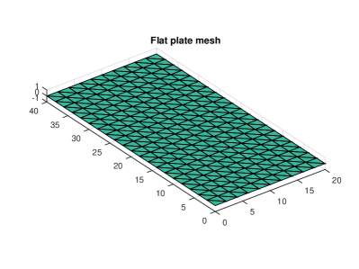
(b)

Figure 1: Model - I: (a) Flat plate example - simply supported on sides $A$ and $D$. The plate is $L=40$ mm long, $H=20$ mm wide, $t=0.8$ mm thick. The Young Modulus is $E=70$ GPa, the Poisson’s ratio is $\nu=0.33$, and the density is $\rho=2700$ Kg/m³. A uniform pressure is applied on the plate, according to the time history $p(t)=P\sin(\omega t)$, where $P=1$ N/mm² and $\omega=2.097\times 10^{4}$ rad/s. (b) The curved plate is discretized using flat, triangular shell elements. The FE mesh contains 400 elements and 1386 DOFs. The two opposite sides parallel to the $y$-axis are simply supported, a uniform pressure is applied on the curved surface, according to the time history.

We consider the rectangular flat plate structure shown in Figure 1. A uniform pressure distribution is chosen to act normal to the plate surface as the external load. A time varying amplitude (load function) is used given by

$$\mathbf{g}(t)=p(t)\mathbf{l},$$

$$p(t)=\sin(\omega t),$$ (43)

where $\mathbf{l}$ is a constant load vector corresponding to a uniform pressure distribution of 1 N/mm². Here, $p(t)$, termed as the dynamic load function, determines the time-dependency of the external load. The results are shown for a periodic choice for $p(t)$ as given by (43), where $\omega$ is chosen to be the first natural frequency of the linearized system. Due to the resonant nature of the dynamics, it is easy to excite geometrically nonlinear behavior in the system, as shown by Figure 2. Furthermore, Figure 2 shows the that the full nonlinear solution is reduced using the QM technique and, subsequently, hyper-reduced using EECSW with good accuracy.

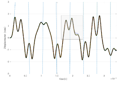
(a)

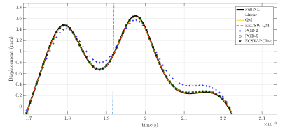
(b)

Figure 2: The linear solution (dashed-blue) grows quickly to high amplitudes for the choice of resonant loading; the full solution (thick black) shows much lower amplitudes due to the geometrical nonlinearities; the ROM obtained using quadratic manifold (yellow) and hyper-reduced solution for this ROM using EECSW (dashed-red) capture the full solution accurately. Subfigure (b) highlights the inaccuracy of the POD ROM with $m=2$.

It can also be confirmed from the global relative error $GRE_{M}$ and speed-up $S^{\star}$, shown in Table 1, that the QM based nonlinear ROM reproduces the results of Model-I with good accuracy but, as expected, does not deliver a good speed-up. The EECSW-based hyper-reduction, on the other hand, gives results with a $GRE_{M}$ of 1.37% but delivers a much higher speed-up of about 100. Note also that a linear-mapping-based ROM with POD of the same size ($m=2$) as the adopted nonlinear mapping does not deliver a good accuracy.

Reduction Technique	Basis size ($m$)	# elements	$GRE_{M}$(%)	$S^{\star}$
POD	2	400	5.62	2.96
POD	5	400	1.81	2.84
ECSW-POD	5	12	2.52	77.7
QM	2	400	1.32	3.03
EECSW-QM	2	6	1.37	99.93

Table 1: Comparison of global relative error $GRE_{M}$ and speed-ups in Model-I for linear-mapping-based ROMs and their hyper-reduced counterparts on one hand, and for quadratic-manifold-based ROMs and their hyper-reduced counterparts using EECSW on the other hand. Time for a full solution run $T_{full}=74.4$ s.

4.3 Wing Structure

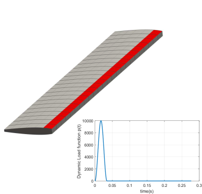
(a)

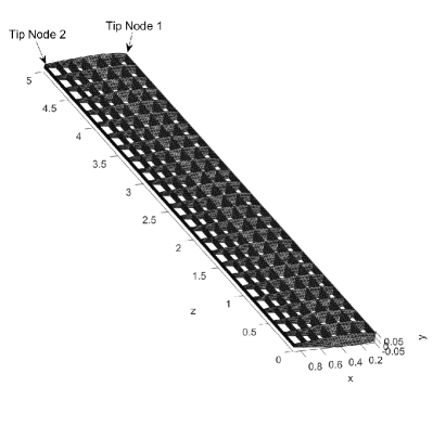
(b)

Figure 3: Model - II: (a) A wing structure with NACA 0012 airfoil (length($L$) = 5 m, Width($W$) $\approx$ 0.9 m, Height($H$) = 0.1 m ) stiffened with ribs along the longitudinal and lateral direction. The Young Modulus is $E=70$ GPa, the Poisson’s ratio is $\nu=0.33$, and the density is $\rho=2700$ Kg/m³. The wing is cantilevered at one end. Uniform pressure is applied on the highlighted area, with a pulse load as given by (44); (b) The structure is meshed with triangular flat shell elements with 6 DOFs per node and each with a thickness of 1.5 mm. The mesh contains $n=135770$ DOFs, $n_{e}=49968$ elements. For illustration purposes, the skin panels are removed, and mesh is shown.

For the application of the proposed extension of EECSW to more realistic models, we consider the model of a NACA-airfoil-based wing structure, introduced in [11]. This model, referred to as Model-II, contains truly high number of DOFs ($n=135770$), thereby, allowing for the appreciation of obtained accuracy and computational speed-ups. We simulate the response of the structure to a low frequency pulse load, applied as a spatially uniform pressure load on the highlighted area on the structure skin (cf. Figure 3). The dynamic load function, shown in Figure 4a, is given as

$$p(t)=A\sin^{2}(\omega t)\left[H(t)-H\left(\frac{\pi}{\omega}-t\right)\right],$$ (44)

where $H(t)$ is the Heaviside function and $\omega$ chosen as the mean of the first and second natural frequency of vibration. We refer the reader to [11] for the detailed linearized, full nonlinear and reduced nonlinear response plots of this model.

Figure 4b and Table 2 show that the hyper-reduction using EECSW for the quadratic-manifold based ROM reproduce the full system response with a very good accuracy ($GRE_{M}\approx 1.71\%$) and is more than a thousand times faster than the full response computation. As expected, we obtain a much higher speed-up during hyper-reduction in comparison with Model-I. The speed-up without hyper-reduction, however, are fairly similar between the two models, despite the striking difference in the number of DOFs. Thus, the numerical results confirm the need and effectiveness of EECSW for hyper-reduction of large nonlinear systems over nonlinear manifolds.

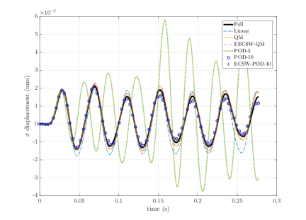
(a)

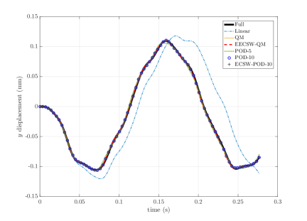
(b)

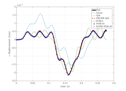
(c)

Figure 4: (a), (b), (c): Comparison of full, linear and various reduced responses at tip node 2 in $x,y$ and $z$ directions. Note that the QM-based reduced solution (with 5 reduced unknowns) accurately captures the full system response, where as the POD-based ROM with 5 modes fails to reproduce the nonlinear system response (POD-5).

Figure 4 and Table 2 compare the response of Model-II to the applied load. Figure 4 further shows that the response of the full system is captured more effectively using the quadratic manifold as compared to the POD with the same number of unknowns (POD-5). This underscores the importance of nonlinear manifolds in model reduction of nonlinear systems. In terms of speed as well, we see in Table 2 that the EECSW method performs better than its linear counterpart.

Reduction Technique	Basis size ($m$)	# elements	$GRE_{M}$(%)	$S^{\star}$
POD	5	49968	5.01	3.07
POD	10	49968	0.98	2.77
ECSW-POD	10	152	1.05	794.6

QM	5	49968	1.65	2.92
EECSW-QM	5	44	1.71	1098

Table 2: Starting with a linear modal superposition with $M=5$ modes (first 5 VMs), reduction techniques as described in Section 4.1 are formulated. Global Relative Error and speed-ups in Model-II for these reduction techniques are tabulated. A total of $n_{t}=200$ training vectors, chosen uniformly from the solution time-span, are used to setup hyper-reduction in ECSW-POD and EECSW-QM. Time for a full solution run $T_{full}=3.808\times 10^{4}$ s.

It is interesting that in this case, EECSW-QM ends up sampling a much smaller set of elements as compared to its linear counterpart EECSW-POD, leading to a higher speed-up. This is not to say that nonlinear-manifold-based hyper-reduction would always outperform its linear mapping counterpart. In fact, for a given basis size ($m$) and same number of elements in the sampled mesh, the EECSW method equipped with nonlinear mapping can be expected to be slower that ECSW-POD approach on two accounts:

1. The additional convective terms in the nonlinear-mapping-based ROM (6) adds to the computational burden in comparison with its linear counterpart (7)

2. The evaluation of the nonlinear mapping (quadratic in this case), is expected to be more expensive that a linear mapping, which boils down to a standard matrix-vector product. Though MATLAB is extremely efficient at performing such matrix-vector products, and hence, in the evaluation of linear mappings, the same cannot be said about our sub-optimal implementation for evaluation of the quadratic mapping at hand.

However, for large nonlinear systems, we expect nonlinear manifolds would require much lesser variables to capture the nonlinear behavior in comparison with linear mappings in order to achieve the desired accuracy (cf. discussion in Introduction). We have attempted to demonstrate this using a simple quadratic manifold on a large system, where only 5 unknowns were required to match the accuracy obtained using 10 POD modes (cf. Table 2 and Figure 4). In our experience, a smaller size reduced system usually leads to a smaller size of reduced mesh during training phase as well. This is intuitively clear since the sNNLS problem 17 has fewer constraints to satisfy. Thus, despite the extra costs mentioned in the two points above, EECSW is capable of producing better computational speed-up when equipped with the proper nonlinear manifold (as also seen in Tables 1 and 2).

5 Conclusion

Nonlinear behavior of large structural systems can often be more effectively reduced using nonlinear manifolds in comparison with linear mappings. Though nonlinear manifolds help in reducing the number of unknowns in a large system, hyper-reduction is further needed to achieve the corresponding computational speed up using such ROMs. In this work, we extended the recently developed ECSW technique to allow for hyper-reduction using smooth nonlinear mappings into the reduced system of unknowns. In doing so, we also showed that the ROM obtained by projection onto the tangent space of the manifold, leads to the preservation of structure and stability properties of the ECSW method.

We demonstrated the EECSW method on two structural dynamics examples by hyper-reduction of a ROM based on the quadratic manifold, whereby better speed and accuracy were obtained using the EECSW method in comparison with ECSW-POD based hyper-reduced models. Since these models were based on von-Karman nonlinearities, the degree of nonlinearity in the examples is expected to be much lower than the nominal thin-walled structures featuring geometrically nonlinear behavior. A quadratic manifold was, therefore, effective in capturing the nonlinear behavior effectively for these structures. However, nonlinear manifolds – possibly constructed from solution databases – would play a crucial role in the effective reduction of models with higher degree of nonlinearities (cf. [9]). EECSW in such cases is expected to play a vital role during the hyper-reduction stage by providing the necessary computational speed-ups.

Furthermore, it is easy to see that the proposed extension is capable of handling parameter-dependence in an analogous manner as the original ECSW. However, before applying hyper-reduction using EECSW, we require parameter-dependent nonlinear manifolds in construction of such ROMs. This is certainly not as straight forward as in the linear mapping context, where reduction bases are sometimes even linearly interpolated. Nonetheless, in data-based approaches, parameter dependence can be included into the manifold learning phase. In particular, the parameters can be explicitly modelled as the known features, apart from the reduced variables which would be identified in the manifold learning procedure. This would directly result in parameter-dependent nonlinear manifolds obtained from data. This underscores the need for manifold learning in model reduction with parameter dependence. Thus, using the EECSW on ROMs based on nonlinear manifolds constructed using manifold-learning techniques forms an essential part of our current and future efforts.

Acknowledgements

The authors acknowledge the support of the Air Force Office of Scientific Research, Air Force Material Command, USAF under Award No.FA9550-16-1-0096. We also thank Ludovic Renson for pointing us to the MATLAB-based tensor product toolbox TPROD.

References

- [1] Chaturantabut, S., Sorensen, D. C. Nonlinear model reduction via discrete empirical interpolation, SIAM Journal on Scientic Computing (2010) 32(5): 2737-2764. DOI: 10.1137/090766498
- [2] Tiso, P., Rixen, D. J. (2013) Discrete Empirical Interpolation Method for Finite Element Structural Dynamics. In: Kerschen G., Adams D., Carrella A. (eds) Topics in Nonlinear Dynamics, Volume 1. Conference Proceedings of the Society for Experimental Mechanics Series, vol 35. Springer, New York, NY. DOI: 10.1007/978-1-4614-6570-6_18
- [3] Chaturantabut, S., Beattie, C., Gugercin, S. Structure-preserving Model Reduction for Nonlinear Port-Hamiltonian Systems arXiv:1601.00527 (2016)
- [4] Barrault, M., Maday, Y., Nguyen, N. C., and Patera, A. T. An “empirical interpolation” method: Application to efficient reduced-basis discretization of partial differential equations, C. R. Math. Acad. Sci. Paris (2004) 339: 667–672. DOI: 10.1016/j.crma.2004.08.006
- [5] Farhat, C., Avery, P., Chapman, T., Cortial, J. Dimensional reduction of nonlinear finite element dynamic models with finite rotations and energy-based mesh sampling and weighting for computational efficiency, International Journal for Numerical Methods in Engineering (2014) 98(9): 625-662. DOI: 10.1002/nme.4668
- [6] Matthies, H.G., Meyer, M., Nonlinear Galerkin methods for the model reduction of nonlinear dynamical systems, Computers Structures (2003) 81(9): 1277-1286.
- [7] Farhat, C., Chapman, T., Avery, P. Structure-preserving, stability, and accuracy properties of the energy-conserving sampling and weighting method for the hyper reduction of nonlinear finite element dynamic models, International Journal for Numerical Methods in Engineering (2015) 102(5): 1077-1110. DOI: 10.1002/nme.4820
- [8] Jain, S., Tiso, P., Haller, G., Exact Nonlinear Model Reduction for a von Karman beam: Slow-Fast Decomposition and Spectral Submanifolds, J. Sound Vib. (2018) 423:195–211. DOI: 10.1016/j.jsv.2018.01.049
- [9] Daniel Millán, D., Arroyo, M. Nonlinear manifold learning for model reduction in finite elastodynamics, Computer Methods in Applied Mechanics and Engineering (2013) 261: 118-131
- [10] Peharz, R., Pernkopf, F. Sparse nonnegative matrix factorization with -constraints. Neurocomputing (2012); 80:38–46. DOI: 10.1016/j.neucom.2011.09.024
- [11] Jain, S., Tiso, P., Rixen, D.J., Rutzmoser, J.B. A Quadratic Manifold for Model Order Reduction of Nonlinear Structural Dynamics, Comput. Struct. (2017), 188: 80-94. DOI: 10.1016/j.compstruc.2017.04.005
- [12] Rutzmoser, J.B., Rixen, D.J., Tiso, P., Jain, S. Generalization of Quadratic Manifolds for Reduced Order Modeling of Nonlinear Structural Dynamics, Comput. Struct. (2017), 192: 196-209. DOI: 10.1016/j.compstruc.2017.06.00
- [13] Lines, L.R., Treitel, S. A review of least-squares inversion and its application to geophysical problems, Geophysical Prospecting (1984) 32(2): 159–186. DOI: 10.1111/j.1365-2478.1984.tb00726.x
- [14] van der Maaten, L., Postma, E., van den Herik, J. Dimensionality Reduction: A Comparative Review, TiCC TR 2009?005(2009), Tilburg University
- [15] Ryckelynck D., A priori hyperreduction method: an adaptive approach, J. Comput. Phys. (2005) 201(1): 346–366. DOI: 10.1016/j.jcp.2004.07.015
- [16] Jain, S., Model Order Reduction for Non-linear Structural Dynamics, Master Thesis (2015), Delft University of Technology. UUID: cb1d7058-2cfa-439a-bb2f-22a6b0e5bb2a
- [17] Jain, S., Tiso, P. Simulation-free hyper-reduction for geometrically nonlinear structural dynamics: A quadratic manifold lifting approach. J. Comput. Nonlinear Dynam. (2018) 13(7), 071003. DOI: 10.1115/1.4040021
- [18] Mignolet, M.P., Przekop, A., Rizzi, S.A., Spottswood, S.M. A review of indirect/non-intrusive reduced order modeling of nonlinear geometric structures. J Sound Vib (2013) 332(10): 2437-2460. DOI: 10.1016/j.jsv.2012.10.017
- [19] Barbič, J., James, D. L. Real-Time Subspace Integration for St. Venant-Kirchhoff Deformable Models. ACM Trans. Graph. (2005) 24(3): 982–990. DOI: 10.1145/1073204.1073300
- [20] Everson, R., Sirovich L. Karhunen-Loeve procedure for gappy data. Journal of the Optical Society of America A (1995) 12(8):1657–1664. DOI: 10.1364/JOSAA.12.001657
- [21] Haller, G. and Ponsioen, S. Exact model reduction by a slow?fast decomposition of nonlinear mechanical systems, Nonlinear Dyn. (2017) 90: 617–647. DOI: 10.1007/s11071-017-3685-9
- [22] Carlberg, K. Bou-Mosleh and Farhat, C. Efficient non-linear model reduction via a least-squares Petrov?Galerkin projection and compressive tensor approximations, Int. J. Numer. Meth. Engng (2011); 86: 155–181. DOI: 10.1002/nme.3050
- [23] Carlberg, K., Farhat, C., Cortial, J. and Amsallem D. The GNAT method for nonlinear model reduction: Effective implementation and application to computational fluid dynamics and turbulent flows, J. Comput. Phys. (2013), 242:623–647. DOI: 10.1016/j.jcp.2013.02.028
- [24] Chapman, T. , Avery, P., Collins, P. and Farhat, C. Accelerated mesh sampling for the hyper reduction of nonlinear computational models, Int. J. Numer. Meth. Engng (2017), 109:1623–1654. DOI: 10.1002/nme.5332
- [25] Rega, G. and Troger, H. Dimension Reduction of Dynamical Systems: Methods, Models, Applications, Nonlinear Dyn. (2005), 41: 1–15. DOI: 10.1007/s11071-005-2790-3
- [26] Ding, Q. and Zhang, K. Order reduction and nonlinear behaviors of a continuous rotor system, Nonlinear Dyn. (2012), 67: 251–262. DOI: 10.1007/s11071-011-9975-8
- [27] Lall, S., Krysl, P. and Marsden, J. Structure-preserving model reduction for mechanical systems, Physica D (2003) 184, pp. 304–318. DOI: 10.1016/S0167-2789(03)00227-6