Evolution of initial discontinuities in the DNLS equation theory

Abstract

We present the full classification of wave patterns evolving from an initial step-like discontinuity for arbitrary choice of boundary conditions at the discontinuity location in the DNLS equation theory. In this non-convex dispersive hydrodynamics problem, solutions of the Whitham modulation equations are mapped to parameters of a modulated wave by two-valued functions what makes situation much richer than that for a convex case of the NLS equation type. In particular, new types of simple-wave-like structures appear as building elements of the whole wave pattern. The developed here theory can find applications to propagation of light pulses in fibers and to the theory of Alfvén dispersive shock waves.

1 Introduction

The problem of classification of wave structures evolving from initial discontinuities has played important role since the classical paper of B. Riemann [1]. Complemented by the jump conditions of W. Rankine [2] and H. Hugoniot [3, 4], it provided a prototypical example of formation of shocks in dispersionless media with small viscosity, and the full classification of possible wave patterns evolving from initial discontinuities with general initial data in adiabatic flows of ideal gas was obtained by N. Kotchine [5]. These results were generalized to the class of so-called genuinely nonlinear hyperbolic systems (see, e.g., [6, 7]), however, situation beyond this class is much more complicated and suffers from ambiguity of possible solutions. One of the methods to remove this ambiguity is introduction of small viscosity into equations followed by taking the limit of zero viscosity. This approach seems very natural from physical point of view since it provides some information on the inner structure of viscous shocks. At the same time, there exists another method of regularization of hydrodynamics-like equations, namely, introduction of small dispersion. Although in this case the limit of zero dispersion does not lead to the same shock structure, this approach is of considerable interest since, on one side, it is related with the theory of dispersive shock waves (DSWs) that finds a number of physical applications (see, e.g., review article [8] and references therein) and, on another hand, there are situations when the regularized equation belongs to the class of completely integrable equations and therefore it admits quite thorough investigation including even cases of non-genuinely nonlinear hyperbolic systems.

The simplest example of dispersive nonlinear evolution equation is apparently the famous KdV equation and in this case the solution of the Riemann problem is extremely simple: A. V. Gurevich and L. P. Pitaevskii showed [9] with the use of Whitham modulation theory [10] that there are only two possible ways of evolution of initial discontinuity—it can evolve into either rarefaction wave or DSW whose parameters can be expressed in explicit analytical form by solving the Whitham equations. This result was obtained without explicit use of the complete integrability of the KdV equation [11], but its extension to the NLS equation became possible [12] only after derivation of the Whitham modulation equations [13, 14] by the methods based on the inverse scattering transform for the NLS equation [15] which means its complete integrability. It was shown in Ref. [12] that the NLS equation evolution of any initial discontinuity leads to a wave pattern consisting of a sequence of building blocks two of which are represented by either the rarefaction wave or the DSW, and they are separated by plateau, or vacuum, or two-phase self-similar solution close to unmodulated nonlinear periodic wave. The rarefaction waves are here self-similar simple wave solutions of the dispersionless limit of the NLS equation (i.e., of the shallow water equations) and DSW is described by a self-similar solution of the Whitham modulation equations. In total, there are six different possible wave patterns that can evolve from a given initial discontinuity. Similar classification of wave patterns was also established for the dispersive shallow water Kaup-Boussinesq equation [16, 17].

For classification of wave patterns arising in solutions of the Riemann problem of the KdV or NLS type, it is important that the corresponding dispersionless limits (Hopf equation or shallow water equations) are represented by the genuinely nonlinear hyperbolic equations. If it is not the case, then the classification of the KdV-NLS type becomes insufficient and it was found that it should include new elements—kinks or trigonometric dispersive shocks—for mKdV [18] and Miyata-Camassa-Choi [19] equations. The mKdV equation is a modification of KdV equation and it also describes a unidirectional propagation of wave with a single field variable, so it can be considered as a simplest example of non-convex dispersive hydrodynamics. In spite of its relative simplicity, the full classification of the wave patterns in the solution of the Riemann problem is much more complicated than that in the KdV equation case and it was achieved in Ref. [20] for the Gardner equation (related with the mKdV equation) with the use of Riemann invariant form of the Whitham modulation equations obtained in Ref. [21]. These results were adapted to mKdV equation in Ref. [22] and for this equation the Whitham modulation equations were obtained by the direct Whitham method in Ref. [23]. Instead of two possible patterns in KdV case, in the mKdV-Gardner case we have eight possible wave structures which depend now not only on the sign of the jump at the discontinuity, but also on the values of wave amplitudes at both its sides. No similar classification has been obtained yet for two-directional waves although important partial results were obtained in Ref. [19] for the Miyata-Camassa-Choi equation. However, this equation is not completely integrable and although the principles of such a classification are the same for completely integrable and non-integrable equations, we prefer here to turn first to the case of completely integrable derivative nonlinear Schrödinger (DNLS) equation when more complete study is possible.

Thus, in this paper, we shall give full solution of the Riemann problem for evolution of initial discontinuities in the theory of the DNLS equation

$$\rmi\Psi_{t}+\frac{1}{2}\Psi_{xx}-\rmi(|\Psi|^{2}\Psi)_{x}=0.$$ (1)

This equation appears in the theory of nonlinear Alfvén waves in plasma physics (see, e.g., [24] and references therein) and in nonlinear optics (see, e.g., [25] and references therein). Its complete integrability was established in [26, 27], periodic solution and Whitham modulation equations were derived in [28, 29]. Partial solution of the Riemann problem was obtained in Ref. [32], however, only in the sector of the NLS equation type structures. Here we develop the method which permits one to predict a wave pattern arising from any given data for an initial discontinuity. The method is quite general and it was applied to the generalized NLS equations [33] with Kerr-type cubic nonlinearity added to (1), what is important for nonlinear optics applications, and to the Landau-Lifshitz equation for magnetics with easy-plane anisotropy [ikcphi-17]. Here we develop a similar theory for the equation (1).

2 Hydrodynamic form of the DNLS equation and dispersion law for linear waves

In many situations, it is convenient to transform the DNLS equation (1) to the so-called hydrodynamic form what is achieved by means of the substitution

$$\Psi(x,t)=\sqrt{\rho(x,t)}\exp\left(\rmi\int^{x}u(x^{\prime},t)\rmd x^{\prime}\right).$$ (2)

After separation of real and imaginary parts, this equation is easily reduced to the system

$$\rho_{t}+\left[\rho\left(u-\frac{3}{2}\rho\right)\right]_{x}=0,$$ (3)

$$u_{t}+uu_{x}-(\rho u)_{x}+\left(\frac{\rho_{x}^{2}}{8\rho^{2}}-\frac{\rho_{xx}}{4\rho}\right)_{x}=0.$$ (4)

These equations can be interpreted as hydrodynamic form of the DNLS equation with Eq. (3) playing the role of the continuity equation and Eq. (4) of the Euler equation for a fluid with depending on the flow velocity “pressure” $\rho u$ and “quantum pressure” represented by the last term. However, one should keep in mind that we are dealing with an anisotropic medium where the flux of mass in (3) does not coincide with the momentum density. As a result, the conservation of momentum equation takes the form

$$[\rho(u-\rho)]_{t}+\left[\rho u^{2}-3u\rho^{2}+2\rho^{3}-\frac{1}{4}\rho(\ln\rho)_{xx}\right]_{x}=0.$$ (5)

This feature of the DNLS equation, which in our case means that the ‘right’ and ‘left’ directions of wave propagation cannot be exchanged by an inversion operation $x\to-x$, can be illustrated by the linear approximation.

Let us consider linear waves propagating along the background flow $(\rho_{0},u_{0})$, that is $\rho=\rho_{0}+\rho^{\prime}$, $u=u_{0}+u^{\prime}$, where $|\rho^{\prime}|\ll\rho_{0}$, $|u^{\prime}|\ll u_{0}$. Linearization with respect to small variables $\rho^{\prime},\,u^{\prime}$ yields the system

$$\eqalign{\rho^{\prime}_{t}+(u_{0}-3\rho_{0})\rho^{\prime}_{x}+\rho_{0}u^{\prime}_{x}=0\cr u^{\prime}_{t}+(u_{0}-\rho_{0})u^{\prime}_{x}-\frac{1}{4\rho_{0}}\rho^{\prime}_{xxx}=0.}$$ (6)

Looking for the plane wave solution $\rho^{\prime},u^{\prime}\propto\exp[\rmi(kx-\omega t)]$, we find that it exists if only the dispersion law

$$\omega(k)=k\left[u_{0}-2\rho_{0}\pm\sqrt{\rho_{0}(\rho_{0}-u_{0})+k^{2}/4}\right]$$ (7)

is fulfilled. In the limit of small wave vectors $k$ we find

$$\omega(k)\approx\left(u_{0}-2\rho_{0}\pm\sqrt{\rho_{0}(\rho_{0}-u_{0})}\right)k\pm\frac{k^{3}}{8\sqrt{\rho_{0}(\rho_{0}-u_{0})}}.$$ (8)

As we see, there are two modes of propagation of linear waves with different absolute values of propagation velocities even for medium at rest with $u_{0}=0$: the initial disturbance decays to two wave packets propagating with different absolute values of group velocities.

Another important feature of the dispersion law (7) is that it leads to modulationally unstable modes with complex $\omega$ for $u_{0}>\rho_{0}$. In this paper, we shall confine ourselves to the stable situations only.

The above properties of the wave propagation in the DNLS equation theory are preserved in the weakly nonlinear cases, that is if we take into account weak nonlinear effects in the above modes with $\rho^{\prime}$ small but finite. Before proceeding to this task, we shall consider in the next section the dispersionless dynamics when the dispersion effects are completely neglected.

3 Dispersionless limit

The nonlinear and dispersive effects have the same order of magnitude, when in Eqs. (3), (4) we have $u^{2}\sim\rho u\sim\rho_{xx}/\rho$, hence the last term in Eq. (4) can be neglected if the variables $\rho$ and $u$ change little on distances $\Delta x\sim 1/\rho$. In this dispersionless approximation, the flow is governed by the equations

$$\eqalign{\rho_{t}+\left[\rho\left(u-\frac{3}{2}\rho\right)\right]_{x}=0,\cr u_{t}+uu_{x}-(\rho u)_{x}=0}$$ (9)

or

$$\left(\begin{array}[]{c}\rho\\ u\\ \end{array}\right)_{t}+\mathbb{A}\left(\begin{array}[]{c}\rho\\ u\\ \end{array}\right)_{x}=0,\quad\mathbb{A}=\left(\begin{array}[]{cc}u-3\rho&\rho\\ -u&u-\rho\\ \end{array}\right).$$ (10)

The characteristic velocities of this system

$$v_{\pm}=u-2\rho\pm\sqrt{\rho(\rho-u)}$$ (11)

coincide, naturally, with the phase velocities $\left.\omega/k\right|_{k\to 0}$ for the dispersion laws (7) in the long wave limit. The system (10) of first-order equations can be easily transformed to a diagonal form

$$\frac{\partial r_{+}}{\partial t}+v_{+}\frac{\partial r_{+}}{\partial x}=0,\quad\frac{\partial r_{-}}{\partial t}+v_{-}\frac{\partial r_{-}}{\partial x}=0$$ (12)

for the Riemann invariants

$$r_{+}=u/2-\rho+\sqrt{\rho(\rho-u)},\quad r_{-}=u/2-\rho-\sqrt{\rho(\rho-u)},$$ (13)

with the velocities (11) expressed in terms of the Riemann invariants as

$$v_{+}=\frac{3}{2}r_{+}+\frac{1}{2}r_{-},\quad v_{-}=\frac{1}{2}r_{+}+\frac{3}{2}r_{-}.$$ (14)

If the solution of Eqs. (12) is known, then the physical variables $\rho,u$ are given by the expressions

$$\rho=\frac{1}{2}(\sqrt{-r_{+}}\pm\sqrt{-r_{-}})^{2},\qquad u=\pm 2\sqrt{r_{+}r_{-}},$$ (15)

where both Riemann invariants are negative: $r_{-}\leq r_{+}\leq 0$.

The Riemann invariants (13) and the characteristic velocities (11) are real for $\rho\geq u$ ($\rho\geq 0$ by definition), that is the inequalities $\rho\geq 0,\rho\geq u$ define the hyperbolicity domain in the plane $(u,\rho)$ of physical variables. Besides that, it is extremely important that the Riemann invariant $r_{+}$ reaches its maximal value $r_{+}=0$ along the $\rho$-axis where $u=0$. It means that its dependence on the physical variables is not monotonous. We say that the $\rho$-axis $u=0$ cuts the hyperbolicity domain into two monotonicity regions $u<0$ and $u>0$. Correspondingly, the dependence of the physical variables on the Riemann invariants is not single-valued—it is two-valued in our case of a single maximum of $r_{+}$, if the solution of our hydrodynamics equations crosses the axis $u=0$. As we shall see, this leads to important consequences in classification of wave structures evolving from initial discontinuities.

Now we turn to derivation of the evolution equations for weakly nonlinear waves with small dispersion.

4 Weakly nonlinear waves with small dispersion

The linear modes correspond to flows with fixed relationship between $\rho^{\prime}$ and $u^{\prime}$ and generalizations of these waves to the nonlinear regime are simple waves with one of the Riemann invariants $r_{\pm}$ constant. In the leading order, when the nonlinear and dispersive corrections are accounted in their main approximations, we can add their effects in the resulting evolution equations. The small dispersive effects are described by the last terms in the dispersion laws (8) that can be transformed to the differential equations for $\rho^{\prime}$ by the replacements $\omega\to\rmi\partial_{t}$, $k\to-\rmi\partial_{x}$:

$$\rho^{\prime}_{t}+\left(u_{0}-2\rho_{0}\pm\sqrt{\rho_{0}(\rho_{0}-u_{0})}\right)\rho^{\prime}_{x}\mp\frac{1}{8\sqrt{\rho_{0}(\rho_{0}-u_{0})}}\rho^{\prime}_{xxx}=0.$$ (16)

Therefore it is enough to consider now the weak nonlinear effects neglecting the dispersion. To simplify the notation, we shall consider waves propagating along a uniform quiescent background with $\rho=\rho_{0}$, $u=u_{0}=0$.

4.1 Kortweg-de Vries mode

At first we shall consider waves with $r_{+}=\mathrm{const}$, and it is easy to find that far enough from a localized wave pulse this Riemann invariant vanishes and the identity $r_{-}=0$ is fulfilled with the accuracy up to the first order of small quantities $\rho^{\prime}$ and $u$. Consequently, the equation for $r_{+}$ is already satisfied with this accuracy and for the waves of density $\rho^{\prime}$ we can substitute $u=0$ into dispersionless expressions (11) and (13) for $r_{-}$ and $v_{-}$, correspondingly, to find

$$r_{-}\approx-2(\rho_{0}+\rho^{\prime}),\qquad v_{-}\approx-3(\rho_{0}+\rho^{\prime}).$$

Thus, dispersionless Hopf equation for this mode obtained from (12) reads

$$\rho^{\prime}_{t}-3(\rho_{0}+\rho^{\prime})\rho^{\prime}_{x}=0,$$

and addition of dispersion term from (16) for lower sign yields the KdV equation

$$\rho^{\prime}_{t}-3(\rho_{0}+\rho^{\prime})\rho^{\prime}_{x}-\frac{1}{8\rho_{0}}\rho^{\prime}_{xxx}=0.$$ (17)

Solution of the Riemann problem for this equation has very simple Gurevich-Pitaevskii type [9].

4.2 Modified Korteweg-de Vries mode

In the mode with $r_{-}=-2\rho_{0}=\mathrm{const}$ we have to make calculations with accuracy up to the second order with respect to $\rho^{\prime}$. The condition $r_{-}=-2\rho_{0}$ gives us the relationship

$$u\approx 2\rho^{\prime}-\frac{\rho^{\prime 2}}{\rho_{0}},$$

and its substitution into expressions (11) and (13) for $r_{+}$ and $v_{+}$ yields with the same accuracy

$$r_{+}\approx-\frac{\rho^{\prime 2}}{2\rho_{0}},\qquad v_{+}\approx-\rho_{0}-\frac{\rho^{\prime 2}}{\rho_{0}}.$$

Hence Eq. (12) for $r_{+}$ reduses to the dispersionless equation for the density

$$\rho^{\prime}_{t}-\left(\rho_{0}+\frac{\rho^{\prime 2}}{\rho_{0}}\right)\rho^{\prime}_{x}=0,$$

and addition of dispersion term from (16) for upper sign yields the mKdV equation

$$\rho^{\prime}_{t}--\left(\rho_{0}+\frac{\rho^{\prime 2}}{\rho_{0}}\right)\rho^{\prime}_{x}+\frac{1}{8\rho_{0}}\rho^{\prime}_{xxx}=0.$$ (18)

For this mode the solution of the Riemann problem [20, 22] is much more complicated and this fact suggests that the Riemann problem for the DNLS equation must differ considerably from that for the NLS equation [12]. To find this solution, we have to obtain the periodic solutions in convenient for us form parameterized by the Riemann invariants of the Whitham modulation equations and to derive these modulation equations. Actually, that was done in Refs. [28, 29], however, for completeness we shall reproduce here briefly these results with some improvements.

5 Periodic solutions of the DNLS equation

The finite-gap integration method (see, e.g., [30]) of finding periodic solutions is based on possibility of representing the DNLS equation (1) as a compatibility condition of two systems of linear equations with a spectral parameter $\lambda$

$$\frac{\partial}{\partial x}\left(\begin{array}[]{c}{\psi}_{1}\\ {\psi}_{2}\\ \end{array}\right)=\mathbb{U}\left(\begin{array}[]{c}{\psi}_{1}\\ {\psi}_{2}\\ \end{array}\right),\quad\frac{\partial}{\partial t}\left(\begin{array}[]{c}{\psi}_{1}\\ {\psi}_{2}\\ \end{array}\right)=\mathbb{V}\left(\begin{array}[]{c}{\psi}_{1}\\ {\psi}_{2}\\ \end{array}\right),$$ (19)

where

$$\mathbb{U=}\left(\begin{array}[]{cc}{F}&{G}\\ {H}&-{F}\\ \end{array}\right)\;,\quad\mathbb{V=}\left(\begin{array}[]{cc}{A}&{B}\\ {C}&-{A}\\ \end{array}\right),$$ (20)

with

$$\eqalign{{F}=-2{\rm i}\lambda^{2},\quad{G}=2\lambda\Psi,\quad{H}=2\lambda\Psi^{*},\\ {A}=-{\rm i}\left(4\lambda^{4}+2\lambda^{2}|\Psi|^{2}\right),\quad{B}=4\lambda^{3}\Psi+\lambda\left({\rm i}\Psi_{x}+2|\Psi|^{2}\Psi\right),\\ {C}=4\lambda^{3}\Psi^{*}-\lambda\left({\rm i}\Psi^{*}_{x}-2|\Psi|^{2}\Psi^{*}\right).}$$ (21)

The compatibility condition of linear systems (19),

$$\mathbb{U}_{t}-\mathbb{V}_{x}+[\mathbb{U},\mathbb{V}]=0,$$ (22)

where $[\cdot,\cdot]$ is a commutator of matrices, is equivalent to the DNLS equation.

If we denote as $(\psi_{1},\psi_{2})$ and $(\bar{\psi_{1}},\bar{\psi}_{2})$ two basis solutions of linear systems (19) and introduce a matrix of ‘squared basis functions’

$$\mathbb{W}=\left(\begin{array}[]{cc}-\rmi f&h\\ h&\rmi f\\ \end{array}\right),$$ (23)

where

$$f=-\frac{\rmi}{2}(\psi_{1}\bar{\psi}_{2}+\psi_{2}\bar{\psi}_{1}),\quad g=\psi_{1}\bar{\psi}_{1},\quad h=-\psi_{2}\bar{\psi}_{2},$$ (24)

then equations for these functions can be written in matrix form

$$\mathbb{W}_{x}=[\mathbb{U},\mathbb{W}],\qquad\mathbb{W}_{t}=[\mathbb{V},\mathbb{W}].$$ (25)

It is known that the characteristic polynomial

$$\mathrm{det}(iw\cdot\mathbb{I}-\mathbb{W})=-w^{2}+f^{2}-gh$$ (26)

does not depend on $t$ and $x$ (in our simple case it can be checked by a simple calculation and the general proof of this theorem can be found, e.g., in appendix B of Ref. [31]). Hence, it defines the curve

$$w^{2}=P(\lambda),\qquad P(\lambda)=f^{2}-gh,$$ (27)

where $P(\lambda)$ depends on $\lambda$ only.

Periodic solutions are distinguished by the condition that $P(\lambda)$ be a polynomial in $\lambda$, and then the structure of the matrix elements (21) suggests that $f,g,h$ must also be polynomials in $\lambda$. The simplest one-phase solution corresponds to the polynomials $f,g,h$ in the form

$$f=\lambda^{4}-f_{1}\lambda^{2}+f_{2},\quad g=\lambda(\lambda^{2}-\mu/2)\Psi,\quad h=\lambda(\lambda^{2}-\mu^{*}/2)\Psi^{*}.$$ (28)

The functions ${f}_{1}(x,t)$, ${f}_{2}(x,t)$, $\mu(x,t)$ and $\mu^{*}(x,t)$ are unknown yet, but we shall see soon that $\mu(x,t)$ and $\mu^{*}(x,t)$ are complex conjugate, whence the notation. Then the polynomial $P(\lambda)$ can be written as

$$P(\lambda)=\prod_{i=1}^{4}\left(\lambda^{2}-\lambda_{i}^{2}\right)=\lambda^{8}-s_{1}\lambda^{6}+s_{2}\lambda^{4}-s_{3}\lambda^{2}+s_{4},$$ (29)

where $s_{i}$ are symmetric functions of the four zeroes $\lambda_{i}^{2}$ of the polynomial,

$$s_{1}=\sum_{i}\lambda_{i}^{2},\quad s_{2}=\sum_{i<j}\lambda_{i}^{2}\lambda_{j}^{2},\quad s_{3}=\sum_{i<j<k}\lambda_{i}^{2}\lambda_{j}^{2}\lambda_{k}^{2},\quad s_{4}=\lambda_{1}^{2}\lambda_{2}^{2}\lambda_{3}^{2}\lambda_{4}^{2},$$ (30)

and the identity (27) yields the conservation laws

$$\eqalign{s_{1}=2f_{1}+\nu,\quad s_{2}=f_{1}^{2}+sf_{2}+\nu(\mu+\mu^{*}),\\ s_{3}=2f_{1}f_{2}-\nu\mu\mu^{*},\quad s_{4}=f_{2}^{2},}$$ (31)

where $\nu=|\Psi|^{2}$. This system permits one to express ${f}_{1}(x,t)$, ${f}_{2}(x,t)$, $\mu(x,t)$ and $\mu^{*}(x,t)$ as functions of $\nu$:

$$f_{1}=(s_{1}-\nu)/2,\qquad f_{2}=\pm\sqrt{s_{4}},$$ (32)

$$\mu,\mu^{*}=\frac{1}{8\nu}\left(4s_{2}\pm 8\sqrt{s_{4}}-(\nu-s_{1})^{2}+i\sqrt{-\mathcal{R}(\nu)}\right),$$ (33)

where the polynomial

$$\eqalign{\mathcal{R}(\nu)=\nu^{4}-4s_{1}\nu^{3}+(6s_{1}^{2}-8s_{2}\pm 48\sqrt{s_{4}})\nu^{2}\\ -(4s_{1}^{3}-16s_{1}s_{2}+64s_{3}\pm 32s_{1}\sqrt{s_{4}})\nu+(-s_{1}^{2}+4s_{2}\pm 8\sqrt{s_{4}})^{2}}$$ (34)

is called a resolvent of the polynomial $P(\lambda)$ since its zeroes $\nu_{i}$ are related with the zeroes $\lambda_{j}$ of $P(\lambda)$ by symmetric formulae: the upper signs ($+$) in (34) corresponds to the zeroes

$$\eqalign{\nu_{1}=(-\lambda_{1}+\lambda_{2}+\lambda_{3}+\lambda_{4})^{2},&\nu_{2}=(\lambda_{1}-\lambda_{2}+\lambda_{3}+\lambda_{4})^{2},\\ \nu_{3}=(\lambda_{1}+\lambda_{2}-\lambda_{3}+\lambda_{4})^{2},&\nu_{4}=(\lambda_{1}+\lambda_{2}+\lambda_{3}-\lambda_{4})^{2},}$$ (35)

and the lower signs ($-$) in equation (34) correspond to the zeroes

$$\eqalign{\nu_{1}=(-\lambda_{1}+\lambda_{2}+\lambda_{3}-\lambda_{4})^{2},&\nu_{2}=(\lambda_{1}-\lambda_{2}+\lambda_{3}-\lambda_{4})^{2},\\ \nu_{3}=(\lambda_{1}+\lambda_{2}-\lambda_{3}-\lambda_{4})^{2},&\nu_{4}=(\lambda_{1}+\lambda_{2}+\lambda_{3}+\lambda_{4})^{2}.\\ }$$ (36)

This can be proved by a simple check of the Viète formulae. In both cases the zeroes are ordered according to $\nu_{1}\leq\nu_{2}\leq\nu_{3}\leq\nu_{4}$ for $\lambda_{1}\leq\lambda_{2}\leq\lambda_{3}\leq\lambda_{4}\leq 0$.

From the components

$$g_{x}=2\rmi Gf+2Fg,\qquad g_{t}=2\rmi Bf+2Ag$$ (37)

of the matrix equations (25) at $\lambda=\mu^{1/2}$ we find that $\mu$ satisfies the equations

$$\mu_{x}=4\rmi\sqrt{P(\mu^{1/2})},\quad\mu_{t}=8\rmi(2f_{1}+\nu)\sqrt{P(\mu^{1/2})}=2s_{1}\mu_{x},$$ (38)

where we have used the first equation (31). Consequently, $\mu$ depends on the phase $\xi=x-Vt$ only, where $V=-2s_{1}=-2\sum\lambda_{i}^{2}$. Then the variable $\nu$ also depends on $\xi$ only. Substitution of $g=\lambda(\lambda^{2}-\mu)\Psi$ into the first equation (37) gives $\Psi_{x}=-4\rmi\Psi(f_{1}-\mu)$, so that $\nu_{x}=4\rmi\nu(\mu-\mu^{*})$, and, with the use of (33), we obtain equation for $\nu$,

$$\frac{d\nu}{d\xi}=\sqrt{-\mathcal{R}(\nu)},\quad\xi=x-Vt,\quad V=-\sum\lambda_{i}^{2}=\frac{1}{4}\sum\nu_{i}.$$ (39)

The real solutions of this equation correspond to oscillations of $\nu$ within the intervals where $-\mathcal{R}(\nu)\geq 0$. We shall discuss two possibilities separately.

(A) At first we shall consider the periodic solution corresponding to oscillations of $\nu$ in the interval

$$\nu_{1}\leq\nu\leq\nu_{2}.$$ (40)

Standard calculation yields after some algebra the solution in terms of Jacobi elliptic functions:

$$\nu=\nu_{2}-\frac{(\nu_{2}-\nu_{1})\mathrm{cn}^{2}(\theta,m)}{1+\frac{\nu_{2}-\nu_{1}}{\nu_{4}-\nu_{2}}\mathrm{sn}^{2}(\theta,m)},$$ (41)

where it is assumed that $\nu(0)=\nu_{1}$, and

$$\theta=\sqrt{(\nu_{3}-\nu_{1})(\nu_{4}-\nu_{2})}\,\xi/2,\qquad m=\frac{(\nu_{4}-\nu_{3})(\nu_{2}-\nu_{1})}{(\nu_{4}-\nu_{2})(\nu_{3}-\nu_{1})},$$ (42)

$\mathrm{cn}$ and $\mathrm{sn}$ being Jacobi elliptic functions. The wavelength of the oscillating function (41) is

$$L=\frac{4K(m)}{\sqrt{(\nu_{3}-\nu_{1})(\nu_{4}-\nu_{2})}}=\frac{K(m)}{\sqrt{(\lambda_{3}^{2}-\lambda_{1}^{2})(\lambda_{4}^{2}-\lambda_{2}^{2})}},$$ (43)

where $K(m)$ is the complete elliptic integral of the first kind.

In the limit $\nu_{3}\to\nu_{2}$ ($m\to 1$) the wavelength tends to infinity and the solution (41) acquires the soliton form

$$\nu=\nu_{2}-\frac{\nu_{2}-\nu_{1}}{\cosh^{2}\theta+\frac{\nu_{2}-\nu_{1}}{\nu_{4}-\nu_{2}}\sinh^{2}\theta}.$$ (44)

This is a “dark soliton” for the variable $\nu$.

The limit $m\to 0$ can be reached in two ways.

(i) If $\nu_{2}\to\nu_{1}$, then the solution transforms into a linear harmonic wave

$$\nu\cong\nu_{2}-\frac{1}{2}(\nu_{2}-\nu_{1})\cos(k\xi),\quad k=\sqrt{(\nu_{3}-\nu_{1})(\nu_{4}-\nu_{1})}.$$ (45)

(ii) If $\nu_{4}=\nu_{3}$ but $\nu_{1}\neq\nu_{2}$, then then we arrive at the nonlinear trigonometric solution:

$$\nu=\nu_{2}-\frac{(\nu_{2}-\nu_{1})\cos^{2}\theta}{1+\frac{\nu_{2}-\nu_{1}}{\nu_{3}-\nu_{2}}\sin^{2}\theta},\quad\theta=\sqrt{(\nu_{3}-\nu_{1})(\nu_{3}-\nu_{2})}\,\xi/2.$$ (46)

If we take the limit $\nu_{2}-\nu_{1}\ll\nu_{3}-\nu_{1}$ in this solution, then we return to the small-amplitude limit (45) with $\nu_{4}=\nu_{3}$. On the other hand, if we take here the limit $\nu_{2}\to\nu_{3}=\nu_{4}$, then the argument of the trigonometric functions becomes small and we can approximate them by the first terms of their series expansions. This corresponds to an algebraic soliton of the form

$$\nu=\nu_{2}-\frac{\nu_{2}-\nu_{1}}{1+(\nu_{2}-\nu_{1})^{2}\xi^{2}/4}.$$ (47)

(B) In the second case, the variable $\nu$ oscillates in the interval

$$\nu_{3}\leq\nu\leq\nu_{4}\;.$$ (48)

Here again, a standard calculation yields

$$\nu=\nu_{3}+\frac{(\nu_{4}-\nu_{3})\mathrm{cn}^{2}(\theta,m)}{1+\frac{\nu_{4}-\nu_{3}}{\nu_{3}-\nu_{1}}\mathrm{sn}^{2}(\theta,m)}$$ (49)

with the same definitions (42) and (43) of $\theta$, $m$, and $L$. In this case we have $\nu(0)=\nu_{4}$. In the soliton limit $\nu_{3}\to\nu_{2}$ ($m\to 1$) we get

$$\nu=\nu_{2}+\frac{\nu_{4}-\nu_{2}}{\cosh^{2}\theta+\frac{\nu_{4}-\nu_{2}}{\nu_{2}-\nu_{1}}\sinh^{2}\theta}.$$ (50)

This is a “bright soliton” for the variable $\nu$.

Again, the limit $m\to 0$ can be reached in two ways.

(i) If $\nu_{4}\to\nu_{3}$, then we obtain a small-amplitude harmonic wave

$$\nu\cong\nu_{3}+\frac{1}{2}(\nu_{4}-\nu_{3})\cos(k\xi),\quad k=\sqrt{(\nu_{3}-\nu_{1})(\nu_{3}-\nu_{2})}.$$ (51)

(ii) If $\nu_{2}=\nu_{1}$, then we obtain another nonlinear trigonometric solution,

$$\nu=\nu_{3}+\frac{(\nu_{4}-\nu_{3})\cos^{2}\theta}{1+\frac{\nu_{4}-\nu_{3}}{\nu_{3}-\nu_{1}}\sin^{2}\theta},\quad\theta=\sqrt{(\nu_{3}-\nu_{1})(\nu_{4}-\nu_{1})}\,\xi/2.$$ (52)

If we assume that $\nu_{4}-\nu_{3}\ll\nu_{4}-\nu_{1}$, then we reproduce the small-amplitude limit (51) with $\nu_{2}=\nu_{1}$. On the other hand, in the limit $\nu_{3}\to\nu_{2}=\nu_{1}$ we obtain the algebraic soliton solution:

$$\nu=\nu_{1}+\frac{\nu_{4}-\nu_{1}}{1+(\nu_{4}-\nu_{1})^{2}\xi^{2}/4}.$$ (53)

For both cases (35), (36) we have the identities

$$m=\frac{(\nu_{4}-\nu_{3})(\nu_{2}-\nu_{1})}{(\nu_{4}-\nu_{2})(\nu_{3}-\nu_{1})}=\frac{(\lambda_{4}^{2}-\lambda_{3}^{2})(\lambda_{2}^{2}-\lambda_{1}^{2})}{(\lambda_{4}^{2}-\lambda_{2}^{2})(\lambda_{3}^{2}-\lambda_{1}^{2})}.$$ (54)

The importance of this form of periodic solutions of our equation is related with the fact that the parameters $\lambda_{j}$, connected with $\nu_{i}$ by the formulae (35), (36), can play the role of Riemann invariants in the Whitham theory of modulations.

6 Whitham modulation equations

In modulated waves the parameters $\lambda_{i}$ become slowly varying functions of the space and time variables and their evolution is governed by the Whitham modulation equations. Whitham showed in Ref. [10] that these equations can be obtained by averaging the conservation laws of the full nonlinear system over fast oscillations (whose wavelength $L$ changes slowly along the total wave pattern). Generally speaking, in cases where the periodic solution is characterized by four parameters, this averaging procedure leads to a system of four equations of the type $\nu_{i,t}+\sum_{j}v_{ij}(\nu_{1},\nu_{2},\nu_{3},\nu_{4})\nu_{j,x}=0$ with 16 entries in the “velocity matrix” $v_{ij}$. However, for the case of completely integrable DNLS equation, this system of four equations reduces to a diagonal Riemann form for the Riemann invariants $\lambda_{i}$’s, similar to what occurs for the usual Riemann invariants of non-dispersive waves (see Eqs. (12)). We shall derive the modulation Whitham equations by the method developed in Refs. [29, 30].

First of all, we notice that with the use of (22) and (37) it is easy to prove the identity

$$\frac{\partial}{\partial t}\left(\sqrt{P(\lambda)}\cdot\frac{G(\lambda)}{g(\lambda)}\right)-\frac{\partial}{\partial x}\left(\sqrt{P(\lambda)}\cdot\frac{B(\lambda)}{g(\lambda)}\right)=0,$$ (55)

where we have introduced under the derivative signs the constant on periodic solutions factor $\sqrt{P(\lambda)}$ to transform the identity (27) to the form

$$\left(\frac{f}{\sqrt{P(\lambda)}}\right)^{2}-\frac{g}{\sqrt{P(\lambda)}}\cdot\frac{h}{\sqrt{P(\lambda)}}=1,$$

so that the right-hand side is independent of the variations of $\lambda_{i}$ in a modulated wave, hence the densities and fluxes in the conservation laws can change due to modulations only, as it should be, and any changes caused by $\lambda$-dependent normalization of the $f,g,h$-functions are excluded. We shall use the equation (55) as the generating function of the conservation laws of the DNLS equation: a series expansion in inverse powers of $\lambda$ gives an infinite number of conservation laws of this completely integrable system.

Substitution of Eqs. (22) and (37) into (55) and its simple transformation gives

$$\frac{\partial}{\partial t}\left(\frac{\sqrt{P(\lambda)}}{\lambda^{2}-\mu}\right)-\frac{\partial}{\partial x}\left[\sqrt{P(\lambda)}\left(2+\frac{s_{1}}{\lambda^{2}-\mu}\right)\right]=0,$$

Averaging of the density and of the flux in this expression over one wavelength $L$

$$L=\oint\frac{\rmd\mu}{4\sqrt{-P(\mu^{1/2})}}$$ (56)

according to the rule

$$\langle\left\{\ldots\right\}\rangle=\int_{0}^{L}\left\{\ldots\right\}\frac{\rmd x}{L}=\frac{1}{L}\oint\left\{\ldots\right\}\frac{\rmd x}{\rmd\mu}\rmd\mu=\frac{1}{L}\oint\left\{\ldots\right\}\frac{\rmd\mu}{4\sqrt{-P(\mu^{1/2})}}$$

yields the generating function of the averaged conservation laws:

$$\eqalign{\frac{\partial}{\partial t}\left[\frac{\sqrt{P(\lambda)}}{L}\oint\frac{\rmd\mu}{4(\lambda^{2}-\mu)\sqrt{-P(\mu^{1/2})}}\right]\\ -\frac{\partial}{\partial x}\left[\sqrt{P(\lambda)}\left(2+\frac{s_{1}}{L}\oint\frac{\rmd\mu}{4(\lambda^{2}-\mu)\sqrt{-P(\mu^{1/2})}}\right)\right]=0.}$$ (57)

The condition that in the limit $\lambda\to\lambda_{i}$ the singular terms cancel yields

$$\eqalign{\oint\frac{d\mu}{4(\lambda^{2}_{i}-\mu)\sqrt{-P(\mu^{1/2})}}\cdot\frac{\partial\lambda^{2}_{i}}{\partial t}\\ -\left(2L+{s_{1}}\oint\frac{d\mu}{4(\lambda_{i}-\mu)\sqrt{-P(\mu^{1/2})}}\right)\cdot\frac{\partial\lambda^{2}_{i}}{\partial x}=0.}$$ (58)

From the definition (56) of $L$ one obtains

$$\oint\frac{d\mu}{4(\lambda^{2}_{i}-\mu)\sqrt{-P(\mu^{1/2})}}=-2\,\frac{\partial L}{\partial\lambda^{2}_{i}},$$

which makes it possible to cast Eq. (58) in the form of a Whitham equation for the variables $\lambda_{i}$:

$$\frac{\partial\lambda_{i}}{\partial t}+v_{i}\frac{\partial\lambda_{i}}{\partial x}=0,$$ (59)

where the Whitham velocities $v_{i}$ are given by

$$v_{i}=-{s_{1}}+\frac{L}{\partial L/\partial\lambda^{2}_{i}},\quad\mbox{for}\quad i=1,2,3,4.$$ (60)

The values $\lambda_{i}$ of the spectral parameters are well-defined Riemann invariants of the Whitham system of modulation equations, however, they do not suit well enough to the problems with matching of modulated cnoidal waves and smooth dispersionless solutions. Therefore it is more convenient to define new set of Whitham invariants by using simple fact that any function of a single argument $\lambda_{i}$ is also a Riemann invariant. We define the new Riemann invariants by the formulae

$$r_{i}=-2\lambda_{i}^{2},\quad i=1,2,3,4.$$ (61)

They are negative and ordered according to $r_{1}\leq r_{2}\leq r_{3}\leq r_{4}\leq 0$ for $\lambda_{1}\leq\lambda_{2}\leq\lambda_{3}\leq\lambda_{4}\leq 0$. The parameters $\nu_{i}$ of the periodic solutions of the DNLS equation are expressed in terms of $r_{i}$ as

$$\eqalign{\nu_{1}=(-\sqrt{-r_{1}}+\sqrt{-r_{2}}+\sqrt{-r_{3}}+\sqrt{-r_{4}})^{2}/2,\\ \nu_{2}=(\sqrt{-r_{1}}-\sqrt{-r_{2}}+\sqrt{-r_{3}}+\sqrt{-r_{4}})^{2}/2,\\ \nu_{3}=(\sqrt{-r_{1}}+\sqrt{-r_{2}}-\sqrt{-r_{3}}+\sqrt{-r_{4}})^{2}/2,\\ \nu_{4}=(\sqrt{-r_{1}}+\sqrt{-r_{2}}+\sqrt{-r_{3}}-\sqrt{-r_{4}})^{2}/2,}$$ (62)

or

$$\eqalign{\nu_{1}=(-\sqrt{-r_{1}}+\sqrt{-r_{2}}+\sqrt{-r_{3}}-\sqrt{-r_{4}})^{2}/2,\\ \nu_{2}=(\sqrt{-r_{1}}-\sqrt{-r_{2}}+\sqrt{-r_{3}}-\sqrt{-r_{4}})^{2}/2,\\ \nu_{3}=(\sqrt{-r_{1}}+\sqrt{-r_{2}}-\sqrt{-r_{3}}-\sqrt{-r_{4}})^{2}/2,\\ \nu_{4}=(\sqrt{-r_{1}}+\sqrt{-r_{2}}+\sqrt{-r_{3}}+\sqrt{-r_{4}})^{2}/2.\\ }$$ (63)

The phase velocity and the wavelength are given by

$$V=\frac{1}{2}\sum_{i=1}^{4}r_{i},\quad L=\frac{2K(m)}{\sqrt{(r_{4}-r_{2})(r_{3}-r_{1})}},\quad m=\frac{(r_{4}-r_{3})(r_{2}-r_{1})}{(r_{4}-r_{2})(r_{3}-r_{1})}.$$ (64)

The Whitham modulation equations read

$$\frac{\partial r_{i}}{\partial t}+v_{i}\frac{\partial r_{i}}{\partial x}=0,\quad i=1,2,3,4,$$ (65)

where the Whitham velocities $v_{i}$ are given by

$$v_{i}=-{s_{1}}-\frac{L}{2\partial L/\partial r_{i}},\quad\mbox{for}\quad i=1,2,3,4,$$ (66)

and substitution of $L$ from (64) gives after simple calculation the following explicit expressions

$$\eqalign{v_{1}=\frac{1}{2}\sum_{i=1}^{4}r_{i}-\frac{(r_{4}-r_{1})(r_{2}-r_{1})K(m)}{(r_{4}-r_{1})K(m)-(r_{4}-r_{2})E(m)},\\ v_{2}=\frac{1}{2}\sum_{i=1}^{4}r_{i}+\frac{(r_{3}-r_{2})(r_{2}-r_{1})K(m)}{(r_{3}-r_{2})K(m)-(r_{3}-r_{1})E(m)},\\ v_{3}=\frac{1}{2}\sum_{i=1}^{4}r_{i}-\frac{(r_{4}-r_{3})(r_{3}-r_{2})K(m)}{(r_{3}-r_{2})K(m)-(r_{4}-r_{2})E(m)},\\ v_{4}=\frac{1}{2}\sum_{i=1}^{4}r_{i}+\frac{(r_{4}-r_{3})(r_{4}-r_{1})K(m)}{(r_{4}-r_{1})K(m)-(r_{3}-r_{1})E(m)},}$$ (67)

where $K(m)$ and $E(m)$ are complete elliptic integrals of the first and second type, respectively.

In a modulated wave representing a dispersive shock wave, the Riemann invariants change slowly with $x$ and $t$. The dispersive shock wave occupies a space interval at whose edges two of the Riemann invariants are equal to each other. The soliton edge corresponds to $r_{3}=r_{2}$ $(m=1)$ and at this edge the Whitham velocities are given by

$$\eqalign{{v_{1}}=\frac{1}{2}(3r_{1}+r_{4}),\quad{v_{4}}=\frac{1}{2}(r_{1}+3r_{4}),\\ {v_{2}}={v_{3}}=\frac{1}{2}(r_{1}+2r_{2}+r_{4}).}$$ (68)

The opposite limit $m=0$ can be obtained in two ways. If $r_{3}=r_{4}$, then we get

$$\eqalign{{v_{1}}=\frac{1}{2}(3r_{1}+r_{2}),\quad{v_{2}}=\frac{1}{2}(r_{1}+3r_{2}),\\ {v_{3}}={v_{4}}=2r_{4}+\frac{(r_{2}-r_{1})^{2}}{2(r_{1}+r_{2}-2r_{4})},}$$ (69)

and if $r_{2}=r_{1}$, then

$$\eqalign{{v_{1}}={v_{2}}=2r_{1}+\frac{(r_{4}-r)^{2}}{2(r_{3}+r_{4}-2r_{1})},\\ {v_{3}}=\frac{1}{2}(3r_{3}+r_{4}),\quad{v_{4}}=\frac{1}{2}(r_{3}+3r_{4}).}$$ (70)

From these equations it is clear that at the edges of the oscillatory zone the Whitham equation for two Riemann invariants coincide with those for the dispersionless equations, that is the oscillatory zone can match at its edges with smooth solutions of the dispersionless equations.

Now we are ready to discuss the key elements from which consists any wave structure evolving from an initial discontinuity.

7 Elementary wave structures

Our aim in this paper is to develop the method of derivation of the asymptotic solution of the DNLS evolution problem for a discontinuous step-like initial conditions

$$\rho(x,0)=\cases{\rho^{L}&for $x<0$\\ \rho^{R}&for $x>0$\\ }\qquad u(x,0)=\cases{u^{L}&for $x<0$\\ u^{R}&for $x>0$\\ }.$$ (71)

As we shall see, evolution of this step-like pulse leads to formation of quite complex wave structures consisting of several simpler elements of simple wave type with only one Riemann invariant changing. Therefore we shall first describe these elements in the present section.

7.1 Rarefaction waves

For smooth enough dependence of wave parameters on $x$ and $t$, we can neglect the dispersion effects and use the dispersionless equations derived in section 3. First of all, we notice that the system (12) has a trivial solution for which $r_{+}=\mathrm{const}$ and $r_{-}=\mathrm{const}$. We shall call such a solution a “plateau” because it corresponds to a uniform flow with constant density and flow velocity given by (15).

The initial conditions (71) do not contain any parameters with dimension of time or length. Therefore solutions of equations (12) can depend on the self-similar variable $\zeta=x/t$ only, that is $r_{\pm}=r_{\pm}(\zeta)$, and then this system reduces to

$$\left({v_{+}}-\zeta\right)\frac{dr_{+}}{d\zeta}=0,\quad\left({v_{-}}-\zeta\right)\frac{dr_{-}}{d\zeta}=0.$$ (72)

Evidently, these equations have solutions with one of the Riemann invariants constant and the other one changes in such a way, that the corresponding velocity equals to $\zeta=x/t$. To be definite, let us consider the solution

$$r_{+}=r_{+}^{0}=\mathrm{const},\qquad v_{-}=\frac{1}{2}r_{+}^{0}+\frac{3}{2}r_{-}=\zeta=\frac{x}{t}.$$ (73)

Consequently, $r_{-}$ depends on $x/t$ as

$$r_{-}(x,t)=-\frac{1}{3}r_{+}^{0}+\frac{2}{3}\cdot\frac{x}{t},$$ (74)

and according to Eqs. (15) the physical variables are given by

$$\eqalign{\rho_{\pm}(x,t)=\frac{1}{2}\left(\sqrt{-r_{+}^{0}}\pm\sqrt{\frac{1}{3}r_{+}^{0}-\frac{2}{3}\cdot\frac{x}{t}}\right)^{2},\\ u_{\pm}(x,t)=\pm 2\sqrt{-r_{+}^{0}\left(\frac{1}{3}r_{+}^{0}-\frac{2}{3}\cdot\frac{x}{t}\right)}.}$$ (75)

Here the single solution (73) of equations written in Riemann form yields two solutions (75) in physical variables which we distinguish by the indices $\pm$. These rarefaction waves match to the plateau solutions at their left and right edges. At both edges the invariant $r_{+}$ has the same value $r_{+}=r_{+}^{0}$ whereas we have $r_{-}=r_{-}^{L}$ at the left boundary and $r_{-}=r_{-}^{R}$ at the right boundary. Correspondingly, the above two solutions match to the values of the density

$$\eqalign{(i)\quad\rho_{+}^{L}=\frac{1}{2}\left(\sqrt{-r_{+}^{0}}+\sqrt{-r_{-}^{L}}\right)^{2},\quad\rho_{+}^{R}=\frac{1}{2}\left(\sqrt{-r_{+}^{0}}+\sqrt{-r_{-}^{R}}\right)^{2},\\ (ii)\quad\rho_{-}^{L}=\frac{1}{2}\left(\sqrt{-r_{+}^{0}}-\sqrt{-r_{-}^{L}}\right)^{2},\quad\rho_{-}^{R}=\frac{1}{2}\left(\sqrt{-r_{+}^{0}}-\sqrt{-r_{-}^{R}}\right)^{2},}$$ (76)

and similar formulae can be written for the flow velocities $u_{\pm}^{L,R}$. The edge points propagate with velocities

$$s^{L}=v_{-}(r_{+}^{0},r_{-}^{L})=\frac{1}{2}r_{+}^{0}+\frac{3}{2}r_{-}^{L},\quad s^{R}=v_{-}(r_{+}^{0},r_{-}^{R})=\frac{1}{2}r_{+}^{0}+\frac{3}{2}r_{-}^{R}.$$ (77)

Since $r_{-}^{R}<r_{+}^{R}=r_{+}^{0}$, we always have $s^{R}<r_{+}^{0}$.

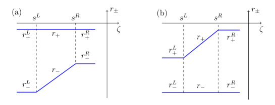
Figure 1: Diagrams of Riemann invariants for the rarefaction wave solutions of the DNLS equation in the dispersionless limit: (a) $r_{+}=\mathrm{const}$; (b) $r_{-}=\mathrm{const}$.

In a similar way we obtain the second solution

$$r_{+}=-\frac{1}{3}r_{-}^{0}+\frac{2}{3}\cdot\frac{x}{t},\quad r_{-}=r_{-}^{0}=\mathrm{const},$$ (78)

hence

$$\eqalign{\rho_{\pm}(x,t)=\frac{1}{2}\left(\sqrt{\frac{1}{3}r_{-}^{0}-\frac{2}{3}\cdot\frac{x}{t}}\pm\sqrt{-r_{-}^{0}}\right)^{2},\\ u_{\pm}(x,t)=\pm 2\sqrt{-r_{-}^{0}\left(\frac{1}{3}r_{-}^{0}-\frac{2}{3}\cdot\frac{x}{t}\right)}.}$$ (79)

In this case we have

$$r_{-}^{0}\leq s^{L}=\frac{3}{2}r_{+}^{L}+\frac{1}{2}r_{-}^{0}<s^{R}=\frac{3}{2}r_{+}^{R}+\frac{1}{2}r_{-}^{0}<\frac{1}{2}r_{-}^{0}.$$ (80)

Diagrams of the Riemann invariants for these rarefaction wave solutions are shown in Fig. 1: the case (a) corresponds to Eqs. (73), (74) and the case (b) to Eqs. (78). Corresponding plots of densities are demonstrated in Fig. 2 by thick lines together with plateau distributions at the edges of the rarefaction waves. Dashed thick lines show both branches of the solutions (75) and (79). It is worth noticing that the edge velocities are determined by the Riemann invariants only and do not depend on the choice of the branch into which the Riemann invariants are mapped.

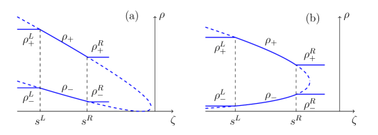
Figure 2: Density distributions in the rarefaction wave solutions of the DNLS equation: (a) $r_{+}=\mathrm{const}$; (b) $r_{-}=\mathrm{const}$.

It is useful to give another graphic representation of the rarefaction waves. From definition (13) of we Riemann invariants we find that they are constant along parabolas

$$\rho=-\frac{1}{2r}\left(\frac{u}{2}-r\right)^{2}$$ (81)

in the $(u,\rho)$-plane, where $r$ is the value of the corresponding Riemann invariant. If a rarefaction wave corresponds to $r_{+}=\mathrm{const}$, then both its left and right points must lie on the same parabola shown in Fig. 3(a) by a blue line. These points can be represented as crossing points of this blue parabola with other two parabolas that represent curves with constant $r_{-}^{L}$ and $r_{-}^{R}$ and are shown by red lines. We have two pairs of “left” and “right” points and obtain, consequently, two types of rarefaction waves described by the diagram Fig. 1(a). These transitions $L_{a}\to R_{a}$ and $L_{b}\to R_{b}$ correspond to different signs in the formulas (75). As we see, both transitions give the growth of $\rho$ with increase of $\zeta$ in agreement with the plots in Fig. 2(a). In a similar way, the situations corresponding to the diagram Fig. 1(b) with constant Riemann invariant $r_{-}$ are represented by the parabolas shown in Fig. 3(b). Now transitions from the “left” points to the “right” ones give the growth of $\rho$ in one case and its decrease in another case, as it is shown in Fig. 2(b). It is important to notice that according to Eq. (75) these transitions connect the points with the same signs of $u$, that is they do not intersect the ordinate axis separating the monotonicity regions. Thus, these rarefaction waves connect the states belonging to the same regions of monotonicity of the Riemann invariants. In the next sections we shall generalize this graphical representation to other wave structures what will be quite helpful in classification of possible wave structures evolving from initial discontinuities.

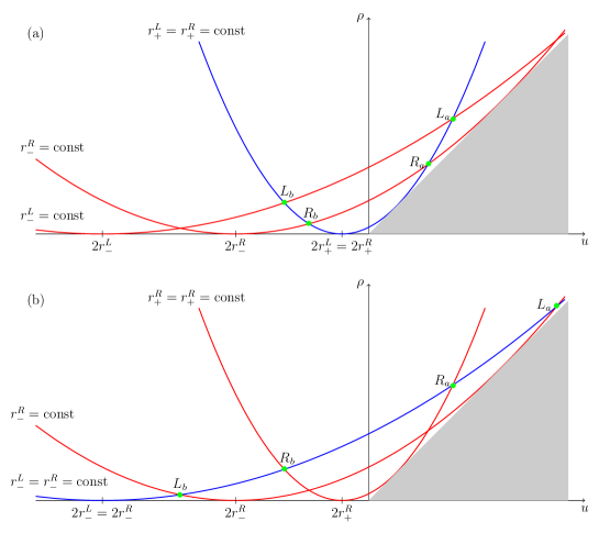
Figure 3: Curves of constant Riemann invariants in the $(u,\rho)$-plane and transitions corresponding to rarefaction waves. Plot (a) represents the rarefaction waves with $r_{+}=\mathrm{const}$ and (b) with $r_{-}=\mathrm{const}$. Grey areas $u>\rho$ correspond to modulationally unstable states with complex characteristic velocities (11).

Both solutions for $\rho_{-}$ can describe flow of liquid into vacuum—in case (75) from left to right and in case (79) from right to left. It is worth noticing a curious particular solution for $u^{L}=0$, when $r_{+}^{0}=0$, $r_{-}=2x/(3t)$ and we get $\rho=-x/(3t)$, $u=0$. It is easy to see that dispersionless equations (9) admit such a solution.

Considered here wave structures satisfy the conditions (a) $r_{+}^{L}=r_{+}^{R}$, $r_{-}^{L}<r_{-}^{R}$ or (b) $r_{+}^{L}<r_{+}^{R}$, $r_{-}^{L}=r_{-}^{R}$. It is natural to ask, what happens if we have the initial conditions satisfying opposite inequalities, and to answer this question we have to consider the DSW structures.

7.2 Cnoidal dispersive shock waves

The other two possible solutions of Eqs. (72) are sketched in Fig. 4, and they satisfy the boundary conditions (a) $r_{+}^{L}=r_{+}^{R}$, $r_{-}^{L}>r_{-}^{R}$ or (b) $r_{+}^{L}>r_{+}^{R}$, $r_{-}^{L}=r_{-}^{R}$. In the dispersionless approximation these multi-valued solutions are nonphysical. However, following to Gurevich and Pitaevskii [9], we can give them clear physical sense by understanding $r_{i}$ as four Riemann invariants of the Whitham system that describe evolution of a modulated nonlinear periodic wave. Naturally, now $r_{i}$ are the self-similar solutions of the Whitham equations (65), that is of the equations

$$(v_{i}-\zeta)\frac{dr_{i}}{d\zeta}=0,\qquad i=1,2,3,4,$$ (82)

which are obvious generalizations of (73):

$$\eqalign{(a)\quad r_{1}=r_{-}^{R},\quad r_{3}=r_{+}^{R},\quad r_{4}=r_{-}^{L},\quad v_{2}(r_{-}^{R},r_{2},r_{-}^{L},r_{+}^{L})=\zeta,\\ (b)\quad r_{1}=r_{-}^{R},\quad r_{2}=r_{+}^{R},\quad r_{4}=r_{+}^{L},\quad v_{3}(r_{-}^{R},r_{+}^{R},r_{3},r_{+}^{L})=\zeta,}$$ (83)

where the last relations determine implicitly dependence of $r_{2}$ and $r_{3}$, correspondingly, on $\zeta$. Sketches of these solutions are shown in Fig. 4. Velocities of the edges of the oscillatory zone whose envelopes are described by the solutions of the Whitham equations are given by

$$\eqalign{(a)&s^{L}=v_{2}(r_{-}^{R},r_{-}^{R},r_{-}^{L},r_{+}^{L})=2r_{-}^{R}+\frac{(r_{+}^{L}-r_{-}^{L})^{2}}{2(r_{+}^{L}+r_{-}^{L}-2r_{-}^{R})},\\ &s^{R}=v_{2}(r_{-}^{R},r_{-}^{L},r_{-}^{L},r_{+}^{L})=\frac{1}{2}(r_{-}^{R}+2r_{-}^{L}+r_{+}^{L}),\\ (b)&s^{L}=v_{3}(r_{-}^{R},r_{+}^{R},r_{+}^{R},r_{+}^{L})=\frac{1}{2}(r_{-}^{R}+2r_{+}^{R}+r_{+}^{L}),\\ &s^{R}=v_{2}(r_{-}^{R},r_{-}^{R},r_{-}^{L},r_{+}^{L})=2r_{-}^{R}+\frac{(r_{+}^{L}-r_{-}^{L})^{2}}{2(r_{+}^{L}+r_{-}^{L}-2r_{-}^{R})},}$$ (84)

correspondingly.

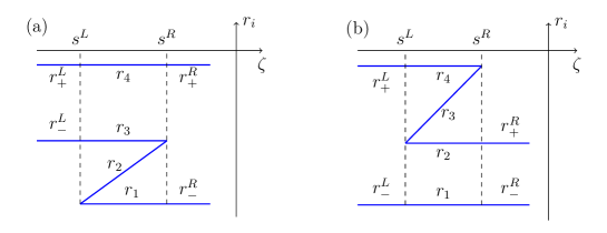
Figure 4: Sketches of Riemann invariants for the DSW solutions of the DNLS equation: (a) $r_{1},r_{3},r_{4}$ are constant and $r_{2}$ is determined by the equation $v_{2}=\zeta$; (b) (a) $r_{1},r_{2},r_{4}$ are constant and $r_{3}$ is determined by the equation $v_{3}=\zeta$.

If we substitute the solutions (83) into formulae (62) and (62), then we determine the dependence of the parameters $\nu_{i}$ on $\zeta$. There are two possibilities shown in Fig. 5: the diagram Fig. 4(a) is mapped by both sets of formulae (62) and (63) into the type Fig. 5(i), whereas the diagram Fig. 4(b) is mapped by the formulae (62) into the type Fig. 5(ii) and by the formulae (63) into the type Fig. 5(i).

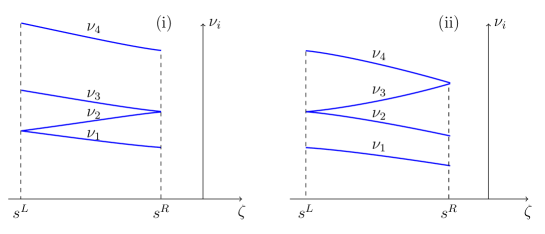
Figure 5: Dependence of the parameters $\nu_{i}$ on $\zeta$ in self-similar solutions of the Whitham equations.

The solutions obtained here are interpreted as formation of cnoidal dispersive shock waves evolving from initial discontinuities with such a type of the boundary conditions. Indeed, Eq. (41) upon substitution of obtained $\nu_{i}$ yields the plots shown in Fig. 6(a)I,II and Fig. 6(b)II, whereas Eq. (49) yields the plot Fig. 6(b)I. We summarize the appearing possibilities in the following list:

• Fig. 4(a) $\stackrel{{\scriptstyle(\ref{312.3a})}}{{\longrightarrow}}$  Fig. 5(i) $\longrightarrow$  Fig. 6(a)    plot I

• Fig. 4(a) $\stackrel{{\scriptstyle(\ref{312.3b})}}{{\longrightarrow}}$  Fig. 5(i) $\longrightarrow$  Fig. 6(a)    plot II

• Fig. 4(b) $\stackrel{{\scriptstyle(\ref{312.3a})}}{{\longrightarrow}}$  Fig. 5(i) $\longrightarrow$  Fig. 6(b)    plot II

• Fig. 4(b) $\stackrel{{\scriptstyle(\ref{312.3b})}}{{\longrightarrow}}$  Fig. 5(ii) $\longrightarrow$  Fig. 6(b)    plot I

As we see, each solution of Whitham equations expressed in terms of Riemann invariants is mapped into two different DSW structures which satisfy the boundary conditions compatible with given values of the Riemann invariants. Such a behavior is typical for non-convex dispersive hydrodynamics and has already been discussed in simpler situation of mKdV (Gardner) equation in Ref. [20].

This two-valued connection of Riemann invariants with solutions in terms of physical variables is similar to the situation described above for the rarefaction waves: the diagram Fig. 1(a) yields two decreasing with $\zeta$ density distributions shown in Fig. 2(a) whereas the diagram Fig. 1(b) yields decreasing and increasing distributions shown in Fig. 2(b). These two types of wave structures will serve us as building blocks appearing in evolution of arbitrary initial discontinuity. It is clear that these cnoidal DSWs are described by the same diagrams of Fig. 3 as the rarefaction waves, but with inverted “left” and “right” points. Hence, the cnoidal DSWs still connect the states belonging to the same regions of monotonicity of the dispersionless Riemann invariants. But there must be waves that connects the states at opposite sides of the $\rho$-axis $u=0$ in the $(u,\rho)$-plane and they also appear as elementary building blocks which are described by the self-similar solutions of the Whitham equations. We shall turn to this type of waves in the next subsection.

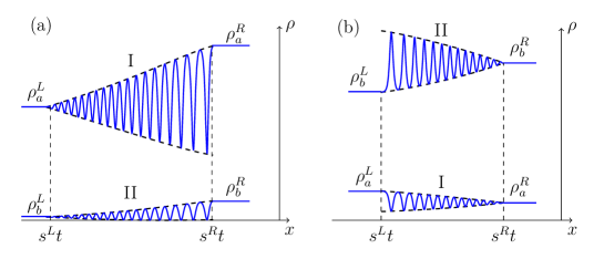
Figure 6: Dispersive shock waves evolved from initial discontinuities for (a) $r^{L}_{+}=r_{4}=r^{R}_{+}$, (b) $r^{L}_{-}=r_{1}=r^{R}_{-}$. The bold dashed lines indicate envelopes of modulated nonlinear waves.

7.3 Trigonometric (contact) dispersive shock waves

At first we shall consider the situation in which the Riemann invariants have equal values at both edges of the shock, i.e., when $r_{-}^{L}=r_{-}^{R}$, $r_{+}^{L}=r_{+}^{R}$. In this case we obtain a new type of wave structure which we shall call a contact dispersive shock wave since it has some similarity with contact discontinuities in the theory of viscous shock waves (see, e.g., [35]). For this situation, the parabolas corresponding to $r_{-}^{L}=\mathrm{const}$ and $r_{-}^{R}=\mathrm{const}$ in Fig. 3(a) coincide with each other and cnoidal DSWs disappear. Instead, there appears the path connecting the identical left and right states labeled by the crossing points of two parabolas as is shown in Fig. 7. Such waves can arise only if the boundary points are located on the opposite sides of the line $u=0$, i.e. in the different regions of monotonicity.

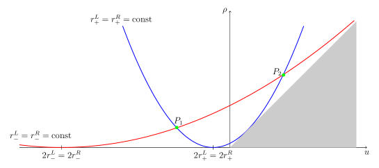
Figure 7: Curves of constant Riemann invariants in the $(u,\rho)$-plane for transitions corresponding to trigonometric dispersive shock waves. The boundary points have identical Riemann invariants $r_{-}^{L}=r_{-}^{R}$, $r_{+}^{L}=r_{+}^{R}$.

Along the arc of the parabola connecting the points $P_{1}$ and $P_{2}$ the two biggest Riemann invariants must be equal to each other, $r_{3}=r_{4}$, and at the left soliton edge they must equal to their boundary value $r_{3}=r_{4}=r_{2}=r_{+}^{L}=r_{+}^{R}$. Hence, we arrive at the diagram of the Riemann invariants shown in Fig. 8. Along this solution we have $m=0$ and the solutions of the Whitham equations is determined by the formula

$$v_{3}=v_{4}=2r_{4}+\frac{(r_{+}^{L}-r_{-}^{L})^{2}}{2(r_{+}^{L}+r_{-}^{L}-2r_{4})}=\zeta$$ (85)

from which we obtain

$$r_{3}=r_{4}=\frac{1}{4}\left[r_{+}^{L}+r_{-}^{L}+\zeta+\sqrt{(r_{+}^{L}+r_{-}^{L}-\zeta)^{2}+2(r_{+}^{L}-r_{-}^{L})^{2}}\right].$$ (86)

At the left soliton edge we have $r_{4}=r_{+}^{L}$ and at the right small-amplitude edge $r_{4}=0$. Therefore Eqs. (69) yields velocities of the edges:

$$s^{L}=\frac{3}{2}r_{+}^{L}+\frac{1}{2}r_{-}^{L},\qquad s^{R}=\frac{(r_{+}^{L}-r_{-}^{L})^{2}}{2(r_{+}^{L}+r_{-}^{L})}.$$ (87)

The sign of the square root in Eq. (86) is chosen in such a way that this formula gives $r_{4}=r_{+}^{L}$ at the left edge with $\zeta=(3r_{+}^{L}+r_{-}^{L})/2$.

Figure 8: Diagram of Riemann invariants for the trigonometric DSW solutions of the DNLS equation.

As one can see from Eqs. (62), in this case $\nu_{3}=\nu_{4}$ and $\nu$ oscillates in the interval $\nu_{1}\leq\nu\leq\nu_{2}$. Then Eq. (46) yields the plot shown in Fig. 9(a) with dark algebraic solitons at the left soliton edge. In case of Eqs. (63) we have $\nu_{1}=\nu_{2}$, hence $\nu$ oscillates in the interval $\nu_{3}\leq\nu\leq\nu_{4}$, and Eq. (52) yields the plot Fig. 9(b) with bright algebraic solitons at the soliton edge. Again the same solution of the Whitham equations represented by a single diagram Fig. 8 is mapped into two different wave structures.

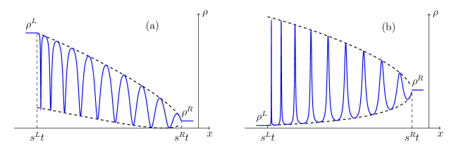
Figure 9: Plots of $\rho$ the trigonometric DSW solutions of the DNLS equation, (a) transition $P_{2}\to P_{1}$, (b) transition $P_{1}\to P_{2}$ in Fig. 7. Dashed thick lines show the envelop functions obtained by solving the Whitham equations.

7.4 Combined shocks

Now we turn to the last elementary wave structures connecting two plateau states. They can also be symbolized by single parabolic arcs between two points in the $(u,\rho)$-plane. This type of paths is illustrated in Fig. 10 and obviously it is a generalization of the preceding structure. In this case, the boundary points are also located in different monotonicity regions. One of the Riemann invariants still remains constant ($r_{-}^{L}=r_{-}^{R}$), however, the boundary values of the other Riemann invariant are different: we have $r_{+}^{L}<r_{+}^{R}$ in case (a) and $r_{+}^{L}>r_{+}^{R}$ in case (b). The corresponding diagrams of Riemann invariants are shown in Fig. 11. As we see, in case (a) the oscillating region located between two plateaus consists of two subregions—one with four different Riemann invariants, what corresponds to a cnoidal DSW, and another one with $r_{3}=r_{4}$, what corresponds to a trigonometric DSW, and there is no any plateau between them. Thus, this diagrams leads to a combined wave structure of “glued” cnoidal and trigonometric DSWs. This structure is illustrated in Fig. 12(a). At the soliton edge the cnoidal DSW matches with the left plateau and the edge with $m=0$ it degenerates into the trigonometric shock. Velocities of the edge points are equal to

$$\eqalign{s_{1}^{L}=v_{3}(r_{-}^{L},r_{+}^{R},r_{+}^{R},r_{+}^{L})=\frac{1}{2}(r_{-}^{L}+2r_{+}^{R}+r_{+}^{L}),\\ s_{2}^{L}=v_{3}(r_{-}^{L},r_{+}^{R},r_{+}^{L},r_{+}^{L})=2r_{+}^{L}+\frac{(r_{+}^{R}-r_{-}^{R})^{2}}{2(r_{+}^{R}+r_{-}^{R}-2r_{+}^{L})},\\ s^{R}=v_{3}(r_{-}^{L},r_{+}^{R},0,0)=\frac{(r_{+}^{R}-r_{-}^{R})^{2}}{2(r_{+}^{R}+r_{-}^{R})}.}$$ (88)

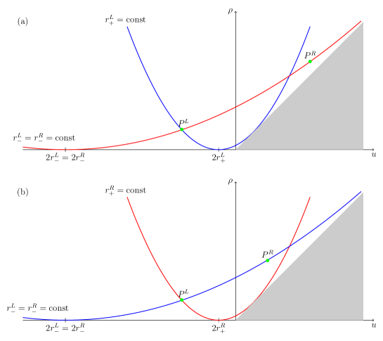
Figure 10: Curves of constant Riemann invariants in the $(u,\rho)$-plane and transitions corresponding to combined waves. Plot (a) represents the rarefaction waves with $r_{+}=\mathrm{const}$ combined with the cnoidal shock and plot (b) corresponds to the trigonometric shock with $r_{-}=\mathrm{const}$ combined with the cnoidal shock.

In a similar way, in case (b) we have a single trigonometric DSW region glued with a rarefaction wave, as is shown in Fig. 12(b). In this case the edge velocities are given by

$$\eqalign{s_{1}^{L}=\frac{1}{2}(3r_{+}^{L}+r_{-}^{L}),\\ s_{2}^{L}=\frac{1}{2}(3r_{+}^{R}+r_{-}^{R}),\\ s^{R}=v_{3}(r_{-}^{L},r_{+}^{R},0,0)=\frac{(r_{+}^{R}-r_{-}^{R})^{2}}{2(r_{+}^{R}+r_{-}^{R})}.}$$ (89)

In both cases, the oscillatory wave is described by the formula (49) or its limit (52) with oscillations of $\nu$ in the interval $\nu_{3}\leq\nu\leq\nu_{4}$.

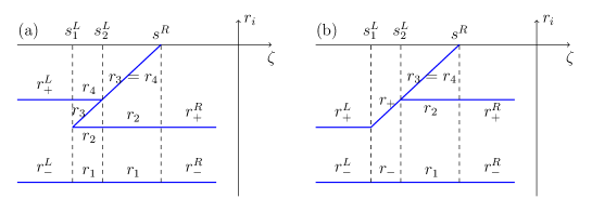
Figure 11: (a) Diagram of the Riemann invariants for the cnoidal shock wave combined with the trigonometric shock wave. (b) Diagram of the Riemann invariants for the rarefaction wave combined with the trigonometric shock wave.

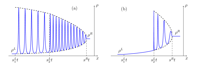
Figure 12: (a) Combined shock wave consisting of the cnoidal and trigonometric dispersive shock waves. (b) Combined shock wave consisting of the rarefaction wave and the trigonometric shock wave.

Now, after description of all elementary wave structures arising in evolution of discontinuities in the DNLS equation theory, we are in position to formulate the main principles of classification of all possible wave structures.

8 Classification of wave patterns

Classification of possible structures is very simple in the KdV equation case when any discontinuity evolves into either rarefaction wave, or cnoidal DSW [9]. It becomes more complicated in the NLS equation case [12] and similar situations as, e.g., for the Kaup-Boussinesq equation [16, 17], where the list consists of eight or ten structures, correspondingly, which can be found after simple enough inspection of available possibilities which are studied one by one. However, the situation changes drastically when we turn to non-convex dispersive hydrodynamics: even in the case of unidirectional Gardner (mKdV) equation we get eight different patterns (instead of two in KdV case) due to appearance of new elements (kinks or trigonometric and combined dispersive shocks), but these patterns can be labeled by two parameters only and therefore these possibilities can be charted on a two-dimensional diagram. In our present case the initial discontinuity (71) is parameterized by four parameters $u^{L},\rho^{L},u^{R},\rho^{R}$, hence the number of possible wave patterns considerably increases and it is impossible to present them in a two-dimensional chart. Therefore it seems more effective to formulate the principles according to which one can predict the wave pattern evolving from a discontinuity with given parameters. Similar method was used [33, 34] in classification of wave patterns evolving from initial discontinuities according to the generalized NLS equation and the Landau-Lifshitz equation for easy-plane magnetics or polarization waves in two-component Bose-Einstein condensate.

We begin with the consideration of the classification problem from the case when both boundary points lie on one side of the axis $u=0$ separating two monotonicity regions in the $(u,\rho)$-plane. At first we shall consider situation when the boundary points lie in the left monotonicity region $u<0$. We show in Fig. 13(a) the two parabolas corresponding to the constant dispersionless Riemann invariants $r_{\pm}^{L}$ related with the left boundary state. Evidently, they cross at some point $L(u^{L},\rho^{L})$ representing the left boundary. These two parabolas cut the left monotonicity region into six domains labeled by the symbols $A,B,\ldots,F$. Depending on the domain, in which the point $R$ with coordinates $(u^{R},\rho^{R})$, representing the right boundary condition, is located, one gets one of the six following possible orderings of the left and right Riemann invariants:

$$\eqalign{\mbox{A}:\quad\lambda_{-}^{R}<\lambda_{+}^{R}<\lambda_{-}^{L}<\lambda_{+}^{L},\\ \mbox{B}:\quad\lambda_{-}^{R}<\lambda_{-}^{L}<\lambda_{+}^{R}<\lambda_{+}^{L},\\ \mbox{C}:\quad\lambda_{-}^{L}<\lambda_{-}^{R}<\lambda_{+}^{R}<\lambda_{+}^{L},\\ \mbox{D}:\quad\lambda_{-}^{R}<\lambda_{-}^{L}<\lambda_{+}^{L}<\lambda_{+}^{R},\\ \mbox{E}:\quad\lambda_{-}^{L}<\lambda_{-}^{R}<\lambda_{+}^{L}<\lambda_{+}^{R},\\ \mbox{F}:\quad\lambda_{-}^{L}<\lambda_{+}^{L}<\lambda_{-}^{R}<\lambda_{+}^{R}.}$$ (90)

All these six domains and corresponding orderings yield six possible wave structures evolving from initial discontinuities. Let us consider briefly each of them.

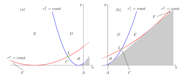
Figure 13: (a) Domains corresponding to different wave structures for evolution on an initial discontinuity whose both edges lie in the left monotonicity region $u<0$. (b) Domains corresponding to different wave structures for evolution on an initial discontinuity whose both edges lie in the right monotonicity region $u>0$.

In case (A) two rarefaction waves are separated by an empty region. Evolution of Riemann invariants and sketch of wave structure are shown in Fig. 14(A).

In case (B) two rarefaction waves are connected by a plateau whose parameters are determined by the dispersionless Riemann invariants $r_{\pm}^{P}$ equal to $r_{-}^{P}=r_{-}^{R}$ and $r_{+}^{P}=r_{+}^{L}$. Here left and right “fluids” flow away from each other with small enough relative velocity and rarefaction waves are able now to provide enough flux to create a plateau in the region between them (see Fig. 14(B)).

In case (C) we obtain a dispersive shock wave on the left side of the structure, a rarefaction wave on its right side and a plateau in between (see Fig. 14(C)).

In case (D) we get the same situation as in the case (C), but now the dispersive shock wave and rarefaction wave exchange their places (see Fig. 14(D)).

In case (E) two DSWs are produced with a plateau between them. Here we have a collision of left and right fluids (see Fig. 14(E)).

In case (F) the plateau observed in the case (E) disappears. It is replaced by a nonlinear wave which can be presented as a non-modulated cnoidal wave (see Fig. 14(F)).

The possible structures for this part of the $(u,\rho)$-plane coincide qualitatively with the patterns found in similar classification problem for the nonlinear Schrödinger equation [12] and this case was already studied in Ref. [32].

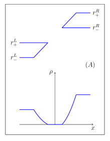
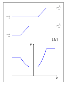
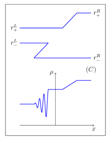
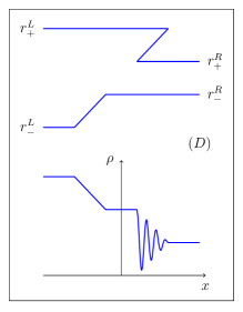
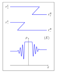
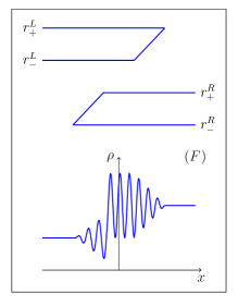
Figure 14: Sketches of behavior of the Riemann invariants and of the corresponding wave structures for six possible choices of the boundary conditions.

If we turn to consideration of the classification problem for the case when both boundary points lie to the right of the line $u=0$, then we get the diagram in the $(u,\rho)$-plane shown in Fig. 13(b). We see that the parabolas cut again this right monotonicity region into six domains. For this case the Riemann invariants can have the same orderings (90) as in the previous case. Depending on the location of the right boundary point in a certain domain, the corresponding wave structure will be formed. Qualitatively these structures coincide with those for the previous case.

At last, we have to study the situation when the boundary points lie on different sides of the line $u=0$, that is in different monotonicity regions. As we have seen in the previous section, in this case new complex structures, namely, combined shocks, appear. It is easy to see that if the left boundary corresponds to the point in the left monotonicity region, then we get again six wave patters, and if it correspond to the point in the right monotonicity region, we get six more patterns, twelve in total. In principle, they can be considered as generalizations of those shown in Fig. 14 with simple elements (rarefaction waves and cnoidal DSWs) replaced by combined shocks. Instead of listing all possible patterns, we shall formulate the general principles of their construction and illustrate them by a typical example. This will provide the method by which one can predict the wave pattern evolving from any given initial discontinuity.

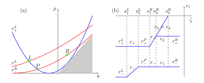
Figure 15: (a) Arcs of parabolas of constant Riemann invariants that join the left $L$ and right $R$ states with plateau $P$ in between. (b) Diagram of Riemenn invariants corresponding to the path in the $(u,\rho)$-plane shown in (a).

For given boundary parameters, we can construct the parabolas corresponding to constant Riemann invariants $r_{\pm}^{L,R}$: each left or right pair of these parabolas crosses at the point $L$ or $R$ representing the left or right boundary state’s plateau. Our task is to construct the path joining these two points, then this path will represent the arising wave structure. We already know the answer for the case when the left and right points lie on the same parabola, see, e.g., Fig. 7. If this is not the case and the right point $R$ lies, say, below the parabola $r_{-}^{L}=\mathrm{const}$, see Fig. 15(a), then we can reach $R$ by means of more complicated path consisting of two arcs of parabolas $LP$ and $PR$ joined at the point $P$. Evidently, this point $P$ represents the plateau between two waves represented by the arcs. At the same time, each arc corresponds to a wave structure discussed in the preceding section. Having constructed a path from the left boundary point to the right one, it is easy to draw the corresponding diagram of Riemann invariants. To construct the wave structure, we use the formulae connecting the zeroes $\nu_{i}$ of the resolvent with the Riemann invariants $r_{i}$ and expressions for the solutions parameterized by $\nu_{i}$. This solves the problem of construction of the wave structure evolving from the initial discontinuity with given boundary conditions. In fact, there are two paths with a single intersection point that join the left and right boundary points and we choose the physically relevant path by imposing the condition that velocities of edges of all regions must increase from left to right.

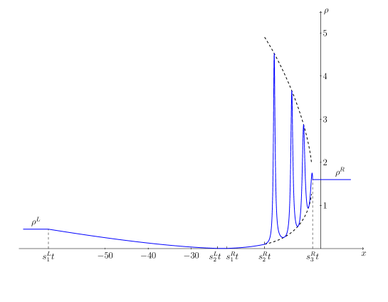
Figure 16: Distribution of $\rho$ in evolutions of the initial discontinuity with $\rho^{L}=0.45$, $u^{L}=-4$, $\rho^{R}=1.6$, $u^{R}=1.5$, what corresponds to the transition $L\to R\in B(u>0)$ as in Fig. 15(a) and the diagram of the Riemann invariants shown in Fig. 15(b). The plateau between two rarefaction waves has the parameters $\rho^{P}=0.005$, $u^{P}=-2.27$. The edge points have velocities $s_{1}^{L}=-6.32$, $s_{2}^{L}=-2.39$, $s_{1}^{R}=-2.18$, $s_{2}^{R}=-1.3$, $s_{3}^{R}=-0.19$. The plot was calculated for $t=10$. Dashed thick lines show envelope functions $\nu_{3}$ and $\nu_{4}$ given by Eqs. (63) for the trigonometric shock with $r_{3}=r_{4}$.

For example, let us consider the case $\rho^{L}=0.45$, $u^{L}=-4$, $\rho^{R}=1.6$, $u^{R}=1.5$ which corresponds to Fig. 15(a) with the transition $L\to R\in B(u>0)$. In this case $r_{-}^{L}=-3.87$, $r_{+}^{L}=-1.035$, $r_{-}^{R}=-1.25$, $r_{+}^{R}=-0.45$ and we see that the arc $PB$ of the parabola with $r_{-}^{R}=\mathrm{const}$ in the above transition crosses the axis $u=0$ as is illustrated in Fig. 15(a). Thus, we arrive at the diagram of Riemann invariants shown in Fig. 15(b). Consequently, at the left edge we have a standard rarefaction wave (the arc $LP$ does not cross the axis $u=0$) and at the right edge the combination of a trigonometric shock with a rarefaction wave. Between these waves we get a plateau characterized by the Riemann invariants $r_{-}^{P}=r_{-}^{R}$ and $r_{+}^{P}=r_{+}^{L}$. This plateau is represented by a single point $P$ in Fig. 15(a). The rarefaction waves are described by the formulas (75) (left wave) and (79) (right wave) with “minus” sight chosen in them. The profile of the oscillatory wave structure can be obtained by substitution of the solution of the Whitham equations

$$r_{1}=r_{-}^{R},\quad r_{2}=r_{+}^{R},\quad v_{3}(r_{-}^{R},r_{+}^{R},r_{3},r_{3})=v_{4}(r_{-}^{R},r_{+}^{R},r_{3},r_{3})=\zeta,$$

into Eq. (52) with $\nu_{i}$ given by Eqs. (63). The velocities of the edge points are equal to

$$\eqalign{s_{1}^{L}=\frac{1}{2}(r_{+}^{L}+3r_{-}^{L}),\quad s_{2}^{L}=\frac{1}{2}(r_{+}^{L}+3r_{-}^{R}),\\ s_{1}^{R}=\frac{1}{2}(3r_{+}^{L}+r_{-}^{R}),\quad s_{2}^{R}=\frac{1}{2}(3r-+^{R}+r_{-}^{R}),\quad s_{3}^{R}=\frac{(r_{+}^{R}-r_{-}^{R})^{2}}{2(r_{+}^{R}+r_{-}^{R})}.}$$

The resulting wave pattern is shown in Fig. 16. It is easy to see, that it represents a deformation of the plot Fig. 14(B): due to crossing the axis $u=0$ the right rarefaction waves acquires a tail in the form of trigonometric DSW. It should be stressed that appearance of such a tail is impossible in the theory of dispersive shock waves in the NLS equation case.

In a similar way we can construct all twelve possible wave patterns for this type on the boundary conditions.

9 Conclusion

In this paper, we have developed the Whitham method of modulations for evolution of waves governed by the DNLS equation. The Riemann problem of evolution of an initial discontinuity is solved for this specific case of non-convex dispersive hydrodynamics. It is found that the set of possible wave structures is much richer than in the convex case (as, e.g., in the NLS equation theory) and includes, as structural elements, trigonometric shock combined with rarefaction waves or cnoidal dispersive shocks. Evolution of these trigonometric shocks is described by the degenerate limits of the Whitham modulation equations. In the resulting scheme, one solution of the Whitham equations corresponds to two different wave patterns, and this correspondence is provided by a two-valued mapping of Riemann invariants to physical modulation parameters. Thus, the algebraic resolvents introduced in Ref. [28] for effectivization of periodic solutions of integrable equations occurred to be crucially important also for establishing the relations between Riemann invariants and modulation parameters of periodic solutions. To determine the pattern evolving from given discontinuity, we have developed a graphical method which is quite flexible and was also applied to other systems with non-convex hydrodynamics—generalized NLS equation for propagation of light pulses in optical fibers [33] and Landau-Lifshitz equation for dynamics of magnetics with uniaxial easy-plane anisotropy [34]. The developed theory can find applications to physics of Alfvén waves in space plasma.

References

References

- [1] Riemann B 1860 Abh. Ges. Wiss. Göttingen, Math.-phys. Kl. 8 43
- [2] Rankine W J M 1870 Phil. Trans. 160 277
- [3] Hugoniot H 1887 Journal de l’École Polytechnique 57 3
- [4] Hugoniot H 1889 Journal de l’École Polytechnique 58 1
- [5] Kotchine N E 1926 Rend. Circ. Matem. Palermo 50 305
- [6] Lax P D 2006 Hyperbolic Partial Differential Equations (New York: AMS)
- [7] Dafermos C M 2010 Hyperbolic Conservation Laws in Continuum Physics (Berlin: Springer)
- [8] El G A and Hoefer M A 2016 Physica D 333 11
- [9] Gurevich A V and Pitaevskii L P 1973 Zh. Eksp. Teor. Fiz. 65 590 [Gurevich A V and Pitaevskii L P 1974 Sov. Phys. JETP 38 291]
- [10] Whitham G B 1965 Proc. Roy. Soc. London, 283 238
- [11] Gardner C S, Greene J M, Kruskal M D, and Miura R M, 1967 Phys. Rev. Lett. 19 1095
- [12] El G A, Geogjaev V V, Gurevich A V, and Krylov A L, (1995) Physica D 87 186
- [13] Forest M G and Lee J E 1986 in Oscillation Theory, Computation and Methods of Compensated Compactness eds Dafermos C, Erickson J L, Kinderlehrer D and Slemrod M, IMA Volumes on Mathematics and its Applications 2 (New York: Springer)
- [14] Pavlov M V 1987 Teor. Mat. Fiz. 71 351 [Pavlov M V 1987 Theor. Math. Phys. 71 584]
- [15] Zakharov V E and Shabat A B 1971 Zh. Exp. Teor. Fiz. 61 118 [Zakharov V E and Shabat A B 1972 Sov. Phys. JETP 34 62]
- [16] El G A, Grimshaw R H J, Pavlov M V 2001 Stud. Appl. Math. 106 157
- [17] Congy T, Ivanov S K, Kamchatnov A M, and Pavloff N 2017 Chaos 27 083107
- [18] Marchant T R 2008 Wave Motion 45 540
- [19] Esler J G and Pearce J D 2011 J. Fluid Mech. 667 555
- [20] Kamchatnov A M, Kuo Y-H, Lin T-C, Horng T-L, Gou S-C, Clift R, El G A, and Grimshaw R H J 2012 Phys. Rev. E 86 036605
- [21] Pavlov M V 1994 Doklady Akad. Nauk 339 157 [Pavlov M V 1995 Russian Acad. Sci. Dokl. Math. 50 400]
- [22] El G A, Hoefer M A, and Shearer M, 2017 SIAM Review 59 3
- [23] Driscoll C F and O’Neil T M 1975 J. Math. Phys. 17 1196
- [24] Kennel C F, Buti B, Hada T, and Pellat R 1988 Phys. Fluids 31 1949
- [25] Akhmanov S A, Vysloukh V A, and Chirkin A S 1986 Usp. Fiz. Nauk 149 449 [Akhmanov S A, Vysloukh V A, and Chirkin A S 1986 Sov. Phys. Uspekhi 1986 29 642l
- [26] Kaup D J and Newell A C 1978 J. Math. Phys. 19 798
- [27] Wadati M, Konno K, and Ichikawa Y H 1979 J. Phys. Soc. Jpn. 46 1698
- [28] Kamchatnov A M 1990 J. Phys. A: Math. Gen.23 2945
- [29] Kamchatnov A M 1990 Zh. Exp. Teor. Fiz. 97 144 [Kamchatnov A M 1990 Sov. Phys. JETP 70 80]
- [30] Kamchatnov A M 2000 Nonlinear Periodic Waves and Their Modulations: An Introductory Course (Singapore: World Scientific)
- [31] Kamchatnov A M 2014 J. Phys. A: Math. Theor. 47 145203
- [32] Gurevich A V, Krylov A L, and El G A 1992 Zh. Exp. Teor. Fiz. 102 1524 [Gurevich A V, Krylov A L, and El G A 1992 Sov. Phys. JETP 75 825]
- [33] Ivanov S K and Kamchatnov A M 2017 Riemann problem for the photon fluid: self-steepening effects, arXiv:1709.04155
- [34] Ivanov S K, Kamchatnov A M, Congy T, and Pavloff N 2017 Solution of the Riemann problem for polarization waves in a two-component Bose-Einstein condensate, arXiv:1709.04193
- [35] Landau L D and Lifshitz E M 1959 Fluid Mechanics (Oxford: Pergamon)