Thermodynamic Bounds on Precision in Ballistic Multi-Terminal Transport

Abstract

For classical ballistic transport in a multi-terminal geometry, we derive a universal trade-off relation between total dissipation and the precision, at which particles are extracted from individual reservoirs. Remarkably, this bound becomes significantly weaker in presence of a magnetic field breaking time-reversal symmetry. By working out an explicit model for chiral transport enforced by a strong magnetic field, we show that our bounds are tight. Beyond the classical regime, we find that, in quantum systems far from equilibrium, correlated exchange of particles makes it possible to exponentially reduce the thermodynamic cost of precision.

Heisenberg’s uncertainty principle is a paradigm example for the ubiquitous interplay between fluctuations and precision. It entails that the accuracy of simultaneous measurements of non-commuting observables is subject to a fundamental lower bound arising from intrinsic fluctuations in the underlying quantum states. Quite remarkably, the precision of non-equilibrium thermodynamic processes might be restricted through thermal fluctuations in a similar way: Barato and Seifert recently suggested that steady-state biomolecular process are subject to a universal trade-off between entropy production and dispersion in the generated output Barato and Seifert (2015). Since its discovery, this thermodynamic uncertainty relation has triggered significant research efforts. A general proof based on methods from large-deviation theory was given by Gingrich et al. for Markov jump processes satisfying a local detailed balance condition Gingrich et al. (2016, 2017). Further developments include extensions to finite-time Pietzonka et al. (2017); Horowitz and Gingrich (2017) and discrete-time Proesmans and Van den Broeck (2017) processes, Brownian clocks Barato and Seifert (2016) and systems obeying Langevin dynamics Hyeon and Hwang (2017); Dechant and Sasa (2017).

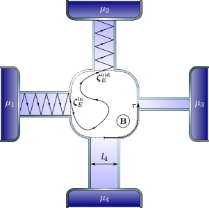
Figure 1: Four-terminal setup as an example for multi-terminal ballistic transport. A two-dimensional target is connected to four reservoirs denoted by their chemical potentials $\mu_{1},\dots,\mu_{4}$ via perfect leads of width $l_{1},\dots,l_{4}$. The solid line crossing the conductor shows the trajectory of a classical particle with energy $E$, which enters the target region at the point $\boldsymbol{\zeta}_{E}^{{{\rm in}}}\equiv(\tau^{{{\rm in}}},p_{\tau}^{{{\rm in}}})$ in the reduced phase space and leaves it at $\boldsymbol{\zeta}^{{{\rm out}}}_{E}\equiv(\tau^{{{\rm out}}},p_{\tau}^{{{\rm out}}})$ after being deflected by the target potential and the magnetic field $\mathbf{B}$. The coordinate $\tau$ parameterizes the boundary of the target region and $p_{\tau}$ denotes the corresponding canonical momentum. Since the particle follows Hamiltonian laws of motion, the scattering map (2) is one-to-one. Because $\tau$ and $p_{\tau}$ are canonical variables, the Poincaré-Cartan theorem implies that this map is also volume preserving Ott (2009).

In light of these results, the question arises, whether a fundamental bound on the precision of thermodynamic processes can be derived from first principles. An ideal stage to investigate this problem is provided by ballistic conductors, that is, devices, whose dimensions are smaller than the mean free path of transport carriers. In such systems, the transfer of particles is governed by reversible laws of motion, while all irreversible effects are relegated to external reservoirs, a mechanism also know as moderate damping Humphrey et al. (2002); Humphrey and Linke (2005). This structural simplicity does not only enable the use of physically transparent models; it also leads to a direct link between micro-dynamics and thermodynamic observables. Features such as the inertia of carriers or Lorentz-type forces, which are not covered by Markov jump processes or overdamped diffusion, are thereby naturally included. These advantages have made ballistic models an important source of insights on classical Stark et al. (2014); Horvat et al. (2009); Casati et al. (2008, 2007) and quantum Brandner et al. (2013); Brandner and Seifert (2013); Sothmann et al. (2014); Brandner and Seifert (2015); Sánchez et al. (2015) transport mechanisms. Here, we use this framework to derive a thermodynamic uncertainty relation for classical ballistic transport, which can be traced back to elementary properties of Hamiltonian dynamics.

Scattering theory provides a powerful tool to describe ballistic transport in both, the classical and the quantum regime. In this approach, the conductor is modeled as a target that is connected to $N$ perfect, effectively infinite leads. Each lead is attached to a reservoir with fully transparent interface injecting thermalized, non-interacting particles. Once inside the conductor, the particles follow deterministic dynamics until they are absorbed again into one of the reservoirs, Fig. 1.

On the classical level, the current flowing in the lead $\alpha$ towards the target corresponds to a phase-space variable $J_{\alpha}[\boldsymbol{\xi}_{t}]$, where the vector $\boldsymbol{\xi}_{t}$ contains the positions and momenta of all particles in the conductor at the time $t$. In the steady state, the mean value and fluctuations of this current are given by

$$J_{\alpha} \equiv\lim_{t\rightarrow\infty}\frac{1}{t}\int_{0}^{t}\!\!\!dt^{\prime}\left\langle J_{\alpha}[\boldsymbol{\xi}_{t^{\prime}}]\right\rangle\quad\text{and}$$ (1)

$$S_{\alpha} \equiv\lim_{t\rightarrow\infty}\frac{1}{t}\int_{0}^{t}\!\!\!dt^{\prime}\!\!\!\int_{0}^{t}\!\!\!dt^{\prime\prime}\left\langle\left(J_{\alpha}[\boldsymbol{\xi}_{t^{\prime}}]-J_{\alpha}\right)\!\left(J_{\alpha}[\boldsymbol{\xi}_{t^{\prime\prime}}]-J_{\alpha}\right)\right\rangle,$$

where the average $\langle\bullet\rangle$ has to be taken over the ensemble of trajectories of injected particles SM .

Exploiting that the injected particles are statistically independent and non-interacting, the expressions (1) can be made more explicit. Focusing on two-dimensional systems from here onwards, to this end, we decompose the trajectory of a single particle with energy $E$ into an incoming and an outgoing part connected by the scattering map

$$\mathcal{S}_{E,\mathbf{B}}:\;\boldsymbol{\zeta}_{E}^{{{\rm in}}}\mapsto\mathcal{S}_{E,\mathbf{B}}[\boldsymbol{\zeta}_{E}^{{{\rm in}}}]=\boldsymbol{\zeta}_{E}^{{{\rm out}}}.$$ (2)

The vectors $\boldsymbol{\zeta}_{E}^{{{\rm in}}}$ and $\boldsymbol{\zeta}_{E}^{{{\rm out}}}$ thereby contain the position and momentum of the particle as it enters and leaves the target region and $\mathbf{B}$ denotes an external magnetic field applied to the target, Fig. 1. Using (2), we further introduce the dimensionless transmission coefficients

$$\mathcal{T}^{\alpha\beta}_{E,\mathbf{B}}=\frac{1}{h}\int_{\beta}\!d\boldsymbol{\zeta}^{{{\rm in}}}_{E}\int_{\alpha}\!d\boldsymbol{\zeta}_{E}\;\delta\bigl{[}\mathcal{S}_{E,\mathbf{B}}[\boldsymbol{\zeta}^{{{\rm in}}}_{E}]-\boldsymbol{\zeta}_{E}\bigr{]},$$ (3)

where indices on integrals imply that the corresponding position variable runs only over the boundary between the target region and the respective lead, $m$ is the mass of a single particle and $h$ Planck’s constant. This definition allows us to compactly rewrite the mean currents and fluctuations (1) as SM

$$J_{\alpha} =\frac{1}{h}\int_{0}^{\infty}\!\!\!dE\;\sum_{\beta}\mathcal{T}^{\alpha\beta}_{E,\mathbf{B}}\bigl{(}u^{\alpha}_{E}-u^{\beta}_{E}\bigr{)}\quad\text{and}$$ (4)

$$S_{\alpha} =\frac{1}{h}\int_{0}^{\infty}\!\!\!dE\sum_{\beta\neq\alpha}\mathcal{T}^{\alpha\beta}_{E,\mathbf{B}}\bigl{(}u^{\alpha}_{E}+u^{\beta}_{E}\bigr{)}.$$

The chemical potentials $\mu_{\alpha}$ and temperature $T$ of the reservoirs enter these expressions via the Maxwell-Boltzmann distributions

$$u^{\alpha}_{E}\equiv\exp\left[-(E-\mu_{\alpha})/(k_{{{\rm B}}}T)\right],$$ (5)

where $k_{{{\rm B}}}$ denotes Boltzmann’s constant. Note that the formulas (4) involve only single-particle quantities, while the original definitions (1) depend on the full phase-space vector $\boldsymbol{\xi}_{t}$ of the many-particle system.

Maintaining the stationary currents $J_{\alpha}$ requires a strictly positive rate of entropy production Seifert (2012); Stark (2013); Stark et al. (2014)

$$\sigma\equiv k_{{{\rm B}}}\sum_{\alpha}\mathcal{F}_{\alpha}J_{\alpha}=\frac{k_{{{\rm B}}}}{h}\int_{0}^{\infty}\!\!\!dE\sum_{\alpha\beta}\mathcal{T}^{\alpha\beta}_{E,\mathbf{B}}\mathcal{F}_{\alpha}\bigl{(}u^{\alpha}_{E}-u^{\beta}_{E}\bigr{)},$$ (6)

which arises due to heat dissipation in the reservoirs. Thus, $\sigma$ can be regarded as the thermodynamic cost of the transport process, which is driven by the dimensionless thermodynamic forces $\mathcal{F}_{\alpha}\equiv(\mu_{\alpha}-\mu)/(k_{{{\rm B}}}T)$ with $\mu$ denoting a reference chemical potential.

We will now show that this cost puts a universal lower bound on the relative uncertainty Barato and Seifert (2015)

$$\varepsilon_{\alpha}\equiv S_{\alpha}/J_{\alpha}^{2}$$ (7)

of each individual current. To this end, we consider the quadratic form

$$A_{\alpha}\equiv\sigma/k_{{{\rm B}}}+2\psi J_{\alpha}x+\psi S_{\alpha}x^{2},$$ (8)

where $x,\psi\in\mathbb{R}$. For systems without an external magnetic field, $A_{\alpha}$ can be written as

$$A_{\alpha}=\sum_{\beta,\gamma\neq\alpha}\!\! \mathcal{V}^{\beta\gamma}\mathcal{D}_{\beta\gamma}\bigl{(}e^{\mathcal{D}_{\beta\gamma}}-1\bigr{)}/2$$ (9)

$$+\sum_{\beta\neq\alpha} \mathcal{V}^{\alpha\beta}\Bigl{\{}\bigl{(}\mathcal{D}_{\alpha\beta}+2\psi x\bigr{)}\bigl{(}e^{\mathcal{D}_{\alpha\beta}}-1\bigr{)}+\psi x^{2}\bigl{(}e^{\mathcal{D}_{\alpha\beta}}+1\bigr{)}\Bigr{\}}$$

with $\mathcal{V}^{\alpha\beta}\equiv\int_{0}^{\infty}\!dE\;\mathcal{T}^{\alpha\beta}_{E}u^{\beta}_{E}/h\geq 0$ and $\mathcal{D}_{\alpha\beta}\equiv\mathcal{F}_{\alpha}-\mathcal{F}_{\beta}$. Here, we used that, at vanishing magnetic field, the transmission coefficients obey $\mathcal{T}^{\alpha\beta}_{E}=\mathcal{T}^{\beta\alpha}_{E}$ as a consequence of time-reversal symmetry Onsager (1931); Casimir (1945); Callen (1985); SM . Next, we observe that, for any $x$, the second sum in (9) is non-negative if $0\leq\psi\leq 2$ . Hence, under this condition, the quadratic form $A_{\alpha}$ is positive semidefinite, since the first sum in (9) is generally non-negative. Consequently, setting $\psi=2$ in (8) and taking the minimum with respect to $x$ yields

$$\sigma\varepsilon_{\alpha}\geq 2k_{{{\rm B}}}.$$ (10)

For systems, where time-reversal symmetry is broken by means of an external magnetic field, the transmission coefficients $\mathcal{T}^{\alpha\beta}_{E,\mathbf{B}}$ are in general not symmetric with respect to $\alpha$ and $\beta$. However, they still fulfill the weaker constraint $\sum_{\beta}\mathcal{T}^{\alpha\beta}_{E,\mathbf{B}}=\sum_{\beta}\mathcal{T}^{\beta\alpha}_{E.\mathbf{B}}$, which follows from the volume-preserving property of the scattering map (2) Stark (2013); Stark et al. (2014); SM . Using this sum rule, the quadratic form (8) can be expressed as

$$A_{\alpha}=\sum_{\beta\neq\alpha}\sum_{\gamma}\mathcal{V}^{\beta\gamma}_{\mathbf{B}}\bigl{(}e^{\mathcal{D}_{\beta\gamma}}-1-\mathcal{D}_{\beta\gamma}\bigr{)}$$ (11)

$$+\sum_{\beta}\mathcal{V}^{\alpha\beta}_{\mathbf{B}}\Bigl{\{}\bigl{(}1+2\psi x\bigr{)}\bigl{(}e^{\mathcal{D}_{\alpha\beta}}-1\bigr{)}+\psi x^{2}\bigl{(}e^{\mathcal{D}_{\alpha\beta}}+1\bigr{)}-\mathcal{D}_{\alpha\beta}\Bigr{\}},$$

where $\mathcal{V}^{\alpha\beta}_{\mathbf{B}}\geq 0$ is defined analogous to $\mathcal{V}^{\alpha\beta}$ in (9). Minimizing the term inside the curly brackets shows that the second sum is (11) is non-negative for any $x$ if

$$0\leq\psi\leq\min_{y\in\mathbb{R}}\frac{(1-e^{y}+ye^{y})(e^{y}+1)}{(e^{y}-1)^{2}}\equiv\psi^{\ast}\simeq 0.89612.$$ (12)

Moreover, the first contribution in (11), which does not depend on $x$, is non-negative due to the convexity of the exponential function. Hence, by using the same argument as in the derivation of (10), we arrive at

$$\sigma\varepsilon_{\alpha}\geq\psi^{\ast}k_{{{\rm B}}}.$$ (13)

The bounds (10) and (13) constitute our first main result. Following from elementary microscopic principles, respectively, time-reversal symmetry and the conservation of phase-space volume, they hold for any scattering potential, any number of terminals and arbitrary far from equilibrium. On the macroscopic level, they imply that any increase in the precision $1/\varepsilon_{\alpha}$, at which particles are extracted from the reservoir $\alpha$, inevitably leads to a proportional increase of the minimal thermodynamic cost $\sigma$ of the transport process. The symmetric bound (10) thereby has exactly the same form as the recently discovered thermodynamic uncertainty relation for Markov jump processes Barato and Seifert (2015); Gingrich et al. (2016, 2017). Remarkably, (13) shows that the minimal cost of precision is reduced by a factor $\psi^{\ast}/2$ in systems, where an external magnetic field breaks the time-reversal symmetry of scattering paths.

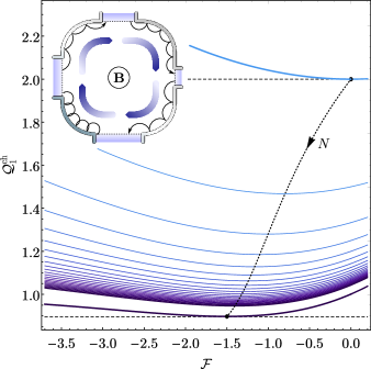
Figure 2: Chiral transport. Bouncing orbits enforced by a strong magnetic field $\mathbf{B}$ sustain clockwise oriented currents between adjacent leads (inset). From top to bottom, the blue blue lines show the cost-precision ratio $\mathcal{Q}_{1}$ defined in (15) as a function of the rescaled bias increment $\mathcal{F}$ for systems with $N=2,\dots,25$ terminals and for the limiting case $N\rightarrow\infty$. Interpolating between the minima of $\mathcal{Q}_{1}$, the dotted line crosses the two dashed lines, respectively indicating the bounds (10) and (13), at $N=2$ and $N\rightarrow\infty$.

To show that our bounds are tight, we consider an $N$-terminal conductor with flat target potential. An external magnetic field $\mathbf{B}$ forces incoming particles with mass $m$ and charge $q$ on bouncing orbits along the boundary of the target region, Fig. 2. This scattering mechanism is captured by the transmission coefficients

$$\mathcal{T}^{\alpha\beta}_{E,\mathbf{B}}=\sqrt{2mE}\bigl{\{}\pi R_{E,\mathbf{B}}\delta_{\alpha\beta-1}+\left(2l_{\alpha}-\pi R_{E,\mathbf{B}}\right)\delta_{\alpha\beta}\bigr{\}}$$ (14)

with periodic indices $\alpha,\beta=1,\dots,N$ Stark et al. (2014). Here, the direction of the magnetic field has been chosen such that the Larmor circles with radius $R_{E,\mathbf{B}}\equiv\sqrt{2mE}/(q|\mathbf{B}|)$ are oriented counterclockwise.

For a strong magnetic field, the typical Larmor radii are small compared to the dimensions of the conductor. Under this condition, the transmission coefficients are given by (14) throughout the relevant range of energies. Due to the asymmetric structure of these coefficients, a chiral steady state emerges, where currents flow in clockwise direction between neighboring reservoirs Sánchez et al. (2015). To generate a net transfer of particles, an external bias has to be applied breaking the $N$-fold rotational symmetry of the system. For simplicity, here we choose the chemical potentials of the reservoirs to increase linearly in steps proportional to $1/N$, that is we set $\mathcal{F}_{\alpha}\equiv\alpha\mathcal{F}/N$. The mean currents and fluctuations can then be evaluated explicitly by inserting (14) into (4). Using the abbreviation $\mathcal{E}\equiv\exp[\mathcal{F}/N]$, we thus obtain the expressions

$$\mathcal{Q}_{1} =\frac{\mathcal{F}}{N}\left\{1+(N-1)\mathcal{E}^{N}-\frac{\mathcal{E}^{N}-1}{\mathcal{E}-1}\right\}\frac{\mathcal{E}+\mathcal{E}^{N}}{(\mathcal{E}-\mathcal{E}^{N})^{2}},$$ (15)

$$\mathcal{Q}_{\alpha} =\frac{\mathcal{F}}{N}\left\{1+(N-1)\mathcal{E}^{N}-\frac{\mathcal{E}^{N}-1}{\mathcal{E}-1}\right\}\frac{\mathcal{E}^{2}+\mathcal{E}}{\mathcal{E}^{\alpha}(\mathcal{E}-1)^{2}}\hskip 13.3103pt(\alpha>1)$$

for the dimensionless product $\mathcal{Q}_{\alpha}\equiv\sigma\varepsilon_{\alpha}/k_{{{\rm B}}}$ of total dissipation (6) and relative uncertainty (7).

In the simplest case $N=2$, the transmission coefficients (14) are still symmetric and (15) reduces to

$$\mathcal{Q}_{\alpha}=\mathcal{F}\coth[\mathcal{F}/4]/2=2+\mathcal{F}^{2}/24+\mathcal{O}\bigl{(}\mathcal{F}^{4}\bigr{)}.$$ (16)

Hence, $\mathcal{Q}_{\alpha}$ reaches its minimum at $\mathcal{F}=0$ and the bound (10) is saturated in the linear response regime. As $N$ increases, the minimum of $\mathcal{Q}_{1}$ becomes successively smaller and shifts to negative values of $\mathcal{F}$, Fig. 2. For large $N$, we obtain the asymptotic expression

$$\bigl{.}\lim_{N\rightarrow\infty}\mathcal{Q}_{1}\bigr{|}_{\mathcal{F}<0}=\frac{(1-e^{\mathcal{F}}+\mathcal{F}e^{\mathcal{F}})(e^{\mathcal{F}}+1)}{(e^{\mathcal{F}}-1)^{2}},$$ (17)

which should be compared with (12). In fact, (17) reaches its minimal value $\psi^{\ast}$ at $\mathcal{F}\simeq-1.49888$. This result shows that the cost-precision ratio $\mathcal{Q}_{1}$ can come arbitrary close to its lower bound (13) as the number of terminals increases. By contrast, $\mathcal{Q}_{\alpha>1}$ asymptotically grows as $N^{2}$ at any $\mathcal{F}\neq 0$. This divergence is a consequence of the chiral transmission coefficients (14) enabling the exchange of particles only between clockwise-adjacent reservoirs: the currents $J_{\alpha>1}$ are effectively driven by the bias $\mathcal{F}/N$ and hence vanish as $1/N$, while the fluctuations $S_{\alpha>1}$ and the total dissipation $\sigma$ stay finite for large $N$.

So far, we have shown that precision in classical ballistic transport requires a minimal thermodynamic cost, which can be substantially reduced in systems with broken time-reversal symmetry. Although our derivations were performed in a 2-dimensional setting, it is straightforward to establish (10) and (13) also in 1 and 3 dimensions. Rather then spelling out the details of this procedure, in the last part of this article, we develop a perspective beyond the classical regime.

For a quantum theory of ballistic transport, the phase-space variable $J_{\alpha}[\boldsymbol{\xi}_{t}]$ in (1) has to be promoted to an operator in the Heisenberg picture. Replacing classical trajectories with quantum states, the ensemble average in (1) can then be evaluated using standard techniques from quantum scattering theory Gaspard (2013, 2015). In this formalism, the crucial role of the scattering map (2) is played by the complex scattering matrices $\mathbf{S}_{E,\mathbf{B}}^{\alpha\beta}$, which connect the amplitudes of incoming waves in the lead $\beta$ and outgoing waves in the lead $\alpha$, respectively Nazarov and Blanter (2009). For fermionic particles, the mean current is thus obtained as

$$J_{\alpha}=\frac{1}{h}\int_{0}^{\infty}\!\!\!dE\sum_{\beta}\hat{\mathcal{T}}^{\alpha\beta}_{E,\mathbf{B}}\bigl{(}f^{\alpha}_{E}-f^{\beta}_{E}\bigr{)}.$$ (18)

Notably, this expression has the same structure as its classical correspondent (4) with the quantum transmission coefficients defined as

$$\hat{\mathcal{T}}^{\alpha\beta}_{E,\mathbf{B}}\equiv 2\;{{{\rm tr}}}\bigl{[}\mathbf{T}_{E,\mathbf{B}}^{\alpha\beta}\bigr{]}\quad\text{with}\quad\mathbf{T}_{E,\mathbf{B}}^{\alpha\beta}\equiv\mathbf{S}^{\alpha\beta}_{E,\mathbf{B}}\bigl{(}\mathbf{S}^{\alpha\beta}_{E,\mathbf{B}}\bigr{)}^{\dagger}$$ (19)

and the Maxwell-Boltzmann distribution (5) replaced by the Fermi-Dirac distribution

$$f^{\alpha}_{E}\equiv 1/\bigl{(}1+\exp[(E-\mu_{\alpha})/(k_{{{\rm B}}}T)]\bigr{)}.$$ (20)

The anatomy of current fluctuations in the quantum regime is, however, more complicated than in the classical case; $S_{\alpha}=S^{{{\rm cl}}}_{\alpha}-S_{\alpha}^{{{\rm qu}}}$ involves two components Nazarov and Blanter (2009)

$$S_{\alpha}^{{{\rm cl}}} \equiv\frac{1}{h}\!\int_{0}^{\infty}\!\!\!dE\sum_{\beta\neq\alpha}\hat{\mathcal{T}}^{\alpha\beta}_{E,\mathbf{B}}\bigl{(}f^{\alpha}_{E}(1-f^{\beta}_{E})+f^{\beta}_{E}(1-f^{\alpha}_{E})\bigl{)},$$ (21)

$$S_{\alpha}^{{{\rm qu}}} \equiv\frac{2}{h}\!\int_{0}^{\infty}\!\!\!dE\sum_{\beta\gamma}{{{\rm tr}}}\bigl{[}\mathbf{T}^{\alpha\beta}_{E,\mathbf{B}}\mathbf{T}^{\alpha\gamma}_{E,\mathbf{B}}\bigr{]}\bigl{(}f^{\alpha}_{E}-f^{\beta}_{E}\bigr{)}\bigl{(}f^{\alpha}_{E}-f^{\gamma}_{E}\bigr{)},$$

both of which are non-negative. Depending only on single-particle quantities, $S^{{{\rm cl}}}_{\alpha}$ can be regarded as the quantum analogue of the classical expression (4) with additional Pauli-blocking factors accounting for the exclusion principle. By contrast, the contribution $S^{{{\rm qu}}}_{\alpha}$, which is of second order in the transmission matrices $\mathbf{T}^{\alpha\beta}_{E,\mathbf{B}}$ and hence describes the correlated exchange of two particles, has no classical counterpart Nazarov and Blanter (2009).

The two-component structure (21) of the current fluctuations suggests to divide the relative uncertainty $\varepsilon_{\alpha}=\varepsilon_{\alpha}^{{{\rm cl}}}-\varepsilon_{\alpha}^{{{\rm qu}}}$ into a quasi-classical part $\varepsilon^{{{\rm cl}}}_{\alpha}\equiv S^{{{\rm cl}}}_{\alpha}/J_{\alpha}^{2}$ and a quantum correction $\varepsilon_{\alpha}^{{{\rm qu}}}\equiv S^{{{\rm qu}}}_{\alpha}/J_{\alpha}^{2}$. By following the lines leading to (10) and (13) it is then possible to establish the bounds SM ; Nenciu (2007)

$$\sigma\varepsilon^{{{\rm cl}}}_{\alpha}\geq 2k_{{{\rm B}}}\quad\text{and}\quad\sigma\varepsilon^{{{\rm cl}}}_{\alpha}\geq\psi^{\ast}k_{{{\rm B}}},$$ (22)

respectively for quantum systems with and without time-reversal symmetry, where $\sigma=k_{{{\rm B}}}\sum_{\alpha}\mathcal{F}_{\alpha}J_{\alpha}$. As in the classical case, this result follows from the symmetry $\hat{\mathcal{T}}^{\alpha\beta}_{E}=\hat{\mathcal{T}}^{\beta\alpha}_{E}$ of the quantum transmission coefficients (19) for $\mathbf{B}=0$ and from the sum rules $\sum_{\beta}\hat{\mathcal{T}}^{\alpha\beta}_{E,\mathbf{B}}=\sum_{\beta}\hat{\mathcal{T}}^{\beta\alpha}_{E,\mathbf{B}}$ for $\mathbf{B}\neq 0$ Nazarov and Blanter (2009). It implies in particular that the classical relations (10) and (13) are recovered close to equilibrium, i.e., for small affinities $\mathcal{F}_{\alpha}$, and in the semi-classical regime, where the fugacities $\varphi_{\alpha}\equiv\exp[\mu_{\alpha}/(k_{{{\rm B}}}T)]$ are small Callen (1985); in both cases the quantum fluctuations $S^{{{\rm qu}}}_{\alpha}$ are negligible.

In general, however, the quantum corrections $\varepsilon^{{{\rm qu}}}_{\alpha}$ will spoil the bounds (10) and (13) as the following simple model shows. Consider a two-terminal conductor with narrow leads allowing only for a single open transport channel, i.e., the system is effectively 1-dimensional and the scattering matrices $\mathbf{S}^{{{\alpha\beta}}}_{E,\mathbf{B}}$ reduce to complex numbers. The target acts as a perfect energy filter, which is fully transparent in a small window $\Delta$ around the reference chemical potential $\mu$ and opaque at all other energies. Such filters are standard tools in mesocopic physics Yamamoto and Hatano (2015); Whitney (2014); Benenti et al. (2017) and can be implemented, for example, with quantum Hall edge states Samuelsson et al. (2017). Setting $\mathcal{F}_{1}\equiv-\mathcal{F}_{2}\equiv\mathcal{F}/2$ and neglecting second-order corrections in $\Delta/(k_{{{\rm B}}}T)$, we obtain

$$\sigma\varepsilon_{\alpha}^{{{\rm cl}}}=k_{{{\rm B}}}\mathcal{F}\coth[\mathcal{F}/2]\;\;\text{and}\;\;\sigma\varepsilon_{\alpha}=k_{{{\rm B}}}\mathcal{F}/\sinh[\mathcal{F}/2]$$ (23)

by evaluating (18) and (21). Hence, while the product of total dissipation $\sigma$ and quasi-classical uncertainty $\varepsilon_{\alpha}^{{{\rm cl}}}$ is bounded by $2k_{{{\rm B}}}$, the full cost-precision ratio $\sigma\varepsilon_{\alpha}$ can become arbitrary small. Specifically, as $\mathcal{F}$ becomes large, the current $J_{\alpha}$ saturates to a finite value, $\sigma$ grows linearly and the fluctuations $S_{\alpha}$ are exponentially suppressed.

This example shows that a combination of quantum effects and energy filtering makes it possible to exponentially reduce the minimal thermodynamic cost of precision. Whether or not this phenomenon can be captured in a generalized trade-off relation, where either cost or precision enters non-linearly, remains an intriguing question for future research. Further prospects include the extension of our theory to systems with temperature gradients or bosonic particles.

Notably, the number $\psi^{\ast}$, which enters the non-symmetric bounds (13) and (22), also appears in a recently found trade-off relation between power and efficiency of stochastic heat engines Shiraishi et al. (2016). These figures are indeed connected with the minimal cost of precision Pietzonka and Seifert (2017). Using our approach, it might thus be possible to bound the performance of ballistic thermoelectric engines, a class of devices that is currently subject to active investigations, see for example Horvat et al. (2009); Saito et al. (2010); Brandner et al. (2013); Brandner and Seifert (2013); Sothmann et al. (2014); Stark et al. (2014); Whitney (2014); Brandner and Seifert (2015); Sánchez et al. (2015); Yamamoto and Hatano (2015); Samuelsson et al. (2017); Benenti et al. (2017). At this point, we conclude by stressing that any violation of our classical bounds constitutes a clear signature of quantum effects. Therefore, our work provides a valuable new benchmark to probe non-classical transport mechanisms in future theoretical and experimental studies.