title
\addtokomafontsection
\addtokomafontsubsection
\addtokomafontsubsubsection
\addtokomafontparagraph
A General Framework for Portfolio Theory. Part II:
drawdown risk measures
Stanislaus Maier-Paape 1 and Qiji Jim Zhu 2 1 Institut für Mathematik, RWTH Aachen, Templergraben 55, D-52062 Aachen, Germany maier@instmath.rwth-aachen.de 2 Department of Mathematics, Western Michigan University, 1903 West Michigan Avenue, Kalamazoo, Michigan, USA qiji.zhu@wmich.edu
Abstract
The aim of this paper is to provide several examples of convex risk measures necessary for the application
of the general framework for portfolio theory of Maier–Paape and Zhu, presented in Part I of this series [12].
As alternative to classical portfolio risk measures such as the standard deviation we in particular construct risk measures
related to the current drawdown of the portfolio equity. Combined with the results of Part I [12],
this allows us to calculate efficient portfolios based on a drawdown risk measure constraint.
Keywords admissible convex risk measures, current drawdown, efficient frontier, portfolio theory,
fractional Kelly allocation, growth optimal portfolio, financial mathematics
Modern portfolio theory due to Markowitz [13] has been the state of the art in mathematical asset allocation for over 50 years.
Recently, in Part I of this series (see Maier–Paape and Zhu [12]), we generalized portfolio theory such that
efficient portfolios can now be considered for a wide range of utility functions and risk measures. The so found portfolios provide an efficient
trade–off between utility and risk just as in the Markowitz portfolio theory. Besides the expected return of the portfolio, which was used by
Markowitz, now general concave utility functions are allowed, e.g. the log utility used for growth optimal portfolio theory
(cf. Kelly [6], Vince [16], [17], Vince and Zhu [19], Zhu [21, 22], Hermes and Maier–Paape [5]).
Growth optimal portfolios maximize the expected log returns of the portfolio yielding fastest compounded growth.
Besides the generalization in the utility functions, as a second breakthrough, more realistic risk measures are now allowed.
Whereas Markowitz and also the related capital market asset pricing model (CAPM) of Sharpe [15] use the standard
deviation of the portfolio return as risk measure, the new theory of Part I in [12] is applicable to a large class
of convex risk measures.
The aim of this Part II is to provide and analyze several such convex risk measures related to the expected log drawdown of the portfolio returns.
Drawdown related risk measures are believed to be superior in yielding risk averse strategies when compared to the standard deviation risk measure.
Furthermore, empirical simulations of Maier–Paape [10] have shown that (drawdown) risk averse strategies are also in great
need when growth optimal portfolios are considered since using them regularly generates tremendous drawdowns (see also van Tharp [20]).
A variety of examples will be provided in Part III [1].
The results in this Part II are a natural generalization of Maier–Paape [11], where drawdown related risk measures for a
portfolio with only one risky asset were constructed. In that paper, as well as here, the construction of randomly drawn equity curves,
which allows the measurement of drawdowns, is given in the framework of the growth optimal portfolio theory (see Section 3 and furthermore
Vince [18].) Therefore, we use Section 2 to provide basics of the growth optimal theory and introduce our setup.
In Section 4 we introduce the concept of admissible convex risk measures, discuss some of their properties and show that the “risk part”
of the growth optimal goal function provides such a risk measure. Then, in Section 5 we apply this concept to the expected log drawdown of the portfolio
returns. It is worth to note that some of the approximations of these risk measures yield, in fact, even positively homogeneous risk measures,
which are strongly related to the concept of deviation measures of Rockafellar, Uryasev and Zabarankin [14]. According to the theory of
Part I [12] such positively homogeneous risk measures provide – as in the CAPM model – an affine structure of the efficient portfolios when the identity utility
function is used. Moreover, often in this situation even a market portfolio, i.e. a purely risky efficient portfolio, related to drawdown risks
can be provided as well.
Finally, note that the main Assumption 2.3 on the trade return matrix of (2.1) together with a no arbitrage
market provides the basic market setup for application of the generalized portfolio theory of Part I [12]. This is shown in the Appendix
(Corollary A.11). In fact, the appendix is used as a link between Part I and Part II and shows how the theory of Part I can
be used with risk measures constructed here. Nonetheless, Parts I and II can be read independently.
Acknowledgement: We thank René Brenner for support in generating the contour plots of the risk measures and Andreas Platen
for careful reading of an earlier version of the manuscript.
2 Setup
For we denote the -th trading system by (system k). A trading system is an investment strategy applied to a
financial instrument. Each system generates periodic trade returns, e.g. monthly, daily or the like. The net trade return of the -th
period of the -th system is denoted
by , . Thus, we have the joint return matrix
and we denote
(2.1)
For better readability, we define the rows of , which represent the returns of the -th period of our systems, as
Following Vince [17], for a vector of portions , where stands for the portion
of our capital invested in (system k), we define the Holding Period Return (HPR) of the -th period as
(2.2)
where is the scalar product in . The Terminal Wealth Relative (TWR) representing the gain (or loss) after the given periods,
when the vector is invested over all periods, is then given as
Since a Holding Period Return of zero for a single period means a total loss of our capital, we restrict to the domain
given by the following definition:
Definition 2.1.
A vector of portions is called admissible if holds, where
Moreover, we define
(2.4)
Note that in particular (the interior of ) and , the boundary of . Furthermore, negative
are in principle allowed for short positions.
Lemma 2.2.
The set in Definition 2.1 is polyhedral and thus convex, as is .
Proof.
For each the condition
defines a half space (which is convex). Since is the intersection of a finite set of half spaces, it is itself convex, in fact even polyhedral.
A similar reasoning yields that is convex, too.
∎
In the following we denote by the unit sphere in , where
denotes the Euclidean norm.
Assumption 2.3.
(no risk free investment)
We assume that the trade return matrix in (2.1) satisfies
(2.5)
In other words, Assumption 2.3 states that no matter what “allocation vector” is
used, there will always be a period resulting in a loss for the portfolio.
Remark 2.4.
(a)
Since implies that , Assumption 2.3
also yields the existence of a period resulting in a gain for each , i.e.
(2.6)
(b)
Note that with Assumption 2.3 automatically follows, i.e. that all
trading systems are linearly independent.
(c)
It is not important whether or not the trading systems are profitable, since we allow short positions
(cf. Assumption 1 in [5]).
Lemma 2.5.
Let the return matrix (as in (2.1)) satisfy Assumption 2.3. Then the set in
(2.1) is compact.
Proof.
Since is closed the lemma follows from (2.5) yielding for sufficiently large.
Thus is bounded as well.
∎
3 Randomly drawing trades
Given a trade return matrix, we can construct equity curves by randomly drawing trades.
Setup 3.1.
(trading game)
Assume trading systems with trade return matrix from (2.1). In a trading game the rows of are drawn randomly.
Each row has a probability of , with . Drawing randomly and independently times from
this distribution results in a probability space
and a terminal wealth relative
(for fractional trading with portion is used)
(3.1)
In the rest of the paper we will use the natural logarithm .
Theorem 3.2.
For each the random variable ,
has expected value
(3.2)
where is the weighted geometric mean of the holding period
returns (see (2.2)) for all .
Proof.
For fixed
holds. For each
is independent of because each is an independent drawing.
We thus obtain
∎
Next we want to split up the random variable into chance and risk parts.
Since corresponds to a winning trade series and
analogously corresponds to a losing trade series we define the random variables corresponding to up trades
and down trades:
As in [11] we next search for explicit formulas for and ,
respectively. By definition
(3.6)
Assume is for the moment fixed and the random variable counts how many
of the are equal to , i.e. if in total of the ’s in are equal to . With similar counting
random variables we obtain integer counts and thus
(3.7)
with obviously . Hence for this fixed we obtain
(3.8)
Therefore the condition on in the sum (3.6) is equivalently expressed as
(3.9)
To better understand the last sum, Taylor expansion may be used exactly as in Lemma 4.5 of [11] to obtain
Lemma 3.5.
Let integers with be given. Let furthermore be a vector of admissible portions where is fixed and .
Then there exists some (depending on and ) such that for all the
following holds:
(a)
(b)
Proof.
The conclusions follow immediately from and .
∎
With Lemma 3.5 we hence can restate (3.9). For and all
the following holds
(3.10)
Note that since is finite and is compact, a (maybe smaller) can be
found such that (3.10) holds for all and .
is clear from (3.3) even for all .
The rest of the proof is along the lines of the proof of the univariate case Theorem 4.6 in [11], but will be given
for convenience. Starting with (3.6) and using (3.7) and (3.10) we get for
Since there are many for which holds we furthermore get from (3.18)
as claimed.
∎
A similar result holds for .
Theorem 3.8.
We assume that the conditions of Theorem 3.7 hold. Then:
(a)
For and
(3.15)
holds, where
(3.16)
(b)
For all and with
(3.17)
i.e. is always an upper bound for the expectation of the down–trade log series.
Remark 3.9.
For large either or or both shall assume
the value in case that at least one of the logarithms in their definition is not defined. Then (3.17)
holds for all .
Proof.
of Theorem 3.8:
ad(a) follows from (3.4) again for all .
Furthermore,
by definition
(3.18)
The arguments given in the proof of Theorem 3.7 apply similarly, where instead of (3.10) we use
Lemma 3.5 (b) to get for
(3.19)
for all with
(3.20)
ad(b)
According to the extension of Lemma 3.5 in Remark 3.6, we also get
(3.21)
for all with (3.20).
Therefore, no matter how large is, the summands of in (3.15) will always contribute
to in (3.18), but — at least for large — there may be even more (negative)
summands from other . Hence (3.17) follows for all .
holds and yields (again) with Theorem 3.7 and 3.8 for
Remark 3.11.
Using Taylor expansion in (3.15) we therefore obtain a first order approximation in of the expected down-trade log series
(3.4), i.e. for and the
following holds:
(3.22)
In the sequel we call the first and the second approximation of the expected down–trade log series.
Noting that for when we extend , we can
improve part (b) of Theorem 3.8:
Corollary 3.12.
In the situation of Theorem 3.8 for all and such that ,
we get:
(a)
(3.23)
(b)
Furthermore is continuous in and (in even positive homogeneous) and
(3.24)
Proof.
(a)
is already clear with the statement above. To show (b), the continuity in of the second approximation
in (3.22) is clear. But even continuity in follows with a short argument:
Using (3.16)
(3.25)
Since is continuous in is
continuous, too, and clearly is non–positive.
∎
4 Admissible convex risk measures
For the measurement of risk, various different approaches have been taken (see for instance [3] for an introduction).
For simplicity, we collect all for us important properties of risk measures in the following three definitions.
Definition 4.1.
(admissible convex risk measure)
Let be a convex set with . A function is called an
admissible convex risk measure (ACRM) if the following properties are satisfied:
(a)
for all .
(b)
is a convex and continuous function.
(c)
For any the function restricted to the set is strictly increasing in ,
and hence in particular for all .
Definition 4.2.
(admissible strictly convex risk measure)
If in the situation of Definition 4.1 the function satisfies only
(a) and (b) but is moreover strictly convex, then is called an
admissible strictly convex risk measure (ASCRM).
Some of the here constructed risk measures are moreover positive homogeneous.
Definition 4.3.
(positive homogeneous)
The risk function is positive homogeneous if
Remark 4.4.
It is easy to see that an admissible strictly convex risk measure automatically satisfies (c) in
Definition 4.1 and thus it is also an admissible convex risk measure.
In fact, if then for some and we obtain for
Examples 4.5.
(a)
The function with , for some symmetric
positive definite matrix is an admissible strictly
convex risk measure (ASCRM).
(b)
For a fixed vector , with for , both,
define admissible convex risk measures (ACRM).
The structure of the ACRM implies nice properties about their level sets:
Lemma 4.6.
Let be an admissible convex risk measure. Then the following holds:
(a)
The set , is convex
and contains .
Furthermore, if is bounded and we have:
(b1)
The boundary of is characterized by
.
(b2)
is a codimension one manifold which varies continuously in .
Proof.
is a convex set, because is a convex function on the convex domain .
Thus (a) is already clear.
ad (b): Assuming is bounded immediately yields
and
, the latter being a codimension
one manifold and continuously varying in due to Definition 4.1(c).
∎
In order to define a nontrivial ACRM, we use the down–trade log series of (3.4).
Theorem 4.7.
For a trading game as in Setup 3.1 satisfying Assumption 2.3 the
function ,
(4.1)
stemming from the down–trade log series in (3.4), is an admissible convex risk measure (ACRM).
Proof.
We show that has the three properties (a), (b), and (c) from
Definition 4.1.
ad (a): is a convex set with according to Lemma 2.2.
Since for all and
and we obtain Definition 4.1(a).
ad (b) For each fixed the function
is continuous in , and therefore the same holds true for . Moreover, again for
fixed, is a concave function of since all summands are as composition of the concave –function with an affine function also concave.
Thus is concave as well since the minimum of two concave functions is still concave and therefore
is convex.
ad (c) It is sufficient to show that
(4.2)
Therefore, let be fixed. In order to show (4) we need to find at least one
such that is
strictly concave in .
Using Assumption 2.3 we obtain some such that .
Hence, for and we obtain
which is a strictly concave function in .
∎
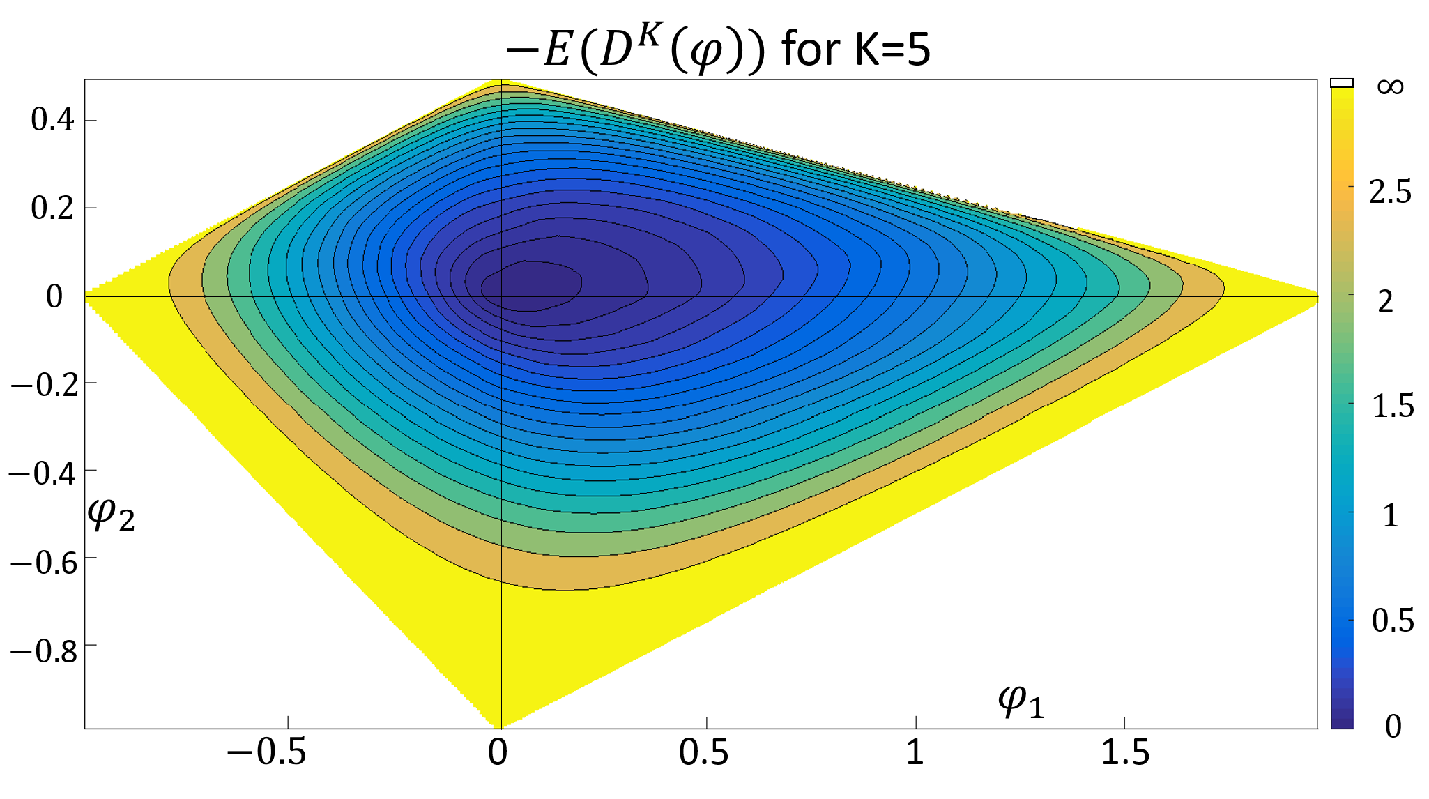
Figure 1: Contour levels for from (4.1)
with for from Example 4.8
Example 4.8.
In order to illustrate of (4.1) and the other risk measures to follow, we introduce a
simple trading game with . Set
(4.7)
It is easy to see that bets in the first system (win with probability or lose ) and bets in the second system
(win with probability or lose ) are stochastically independent and have the same expectation value .
The contour levels of for are shown in Figure 1.
Remark 4.9.
The function in (4.1) may or may not be an admissible strictly convex risk measure.
To show that we give two examples:
(a) For
the risk measure in (4.1) for is not strictly convex. Consider for example
for some fixed .
Then for small, in the trading game only the third row results
in a loss, i.e.
which is constant along the line
for small and thus not strictly convex.
(b) We refrain from giving a complete characterization for trade return matrices for which (4.1)
results in a strictly convex function, but only note that if besides Assumption 2.3 the condition
(4.8)
then this is sufficient to give strict convexity of (4.1) and hence in this case in (4.1)
is actually an ASCRM.
Now that we saw that the negative expected down–trade log series of (4.1) is an admissible convex risk measure,
it is natural to ask whether or not the same is true for the two approximations of the expected down–trade log series
given in (3.15) and (3.22) as well. Starting with
from (3.15), the answer is negative.
The reason is simply that from (3.16) is in general not continuous for such for which
with exist and which satisfy , but unlike in (3) for , the sum over the log terms
may not vanish.
Therefore is
in general also not continuous. A more thorough discussion of this discontinuity can be found after Theorem 4.10.
On the other hand, of (3.22) was proved to be continuous and non–positive
in Corollary 3.12. In fact, we can obtain:
Theorem 4.10.
For the trading game of Setup 3.1 satisfying Assumption 2.3 the function ,
(4.9)
with from (3) is an admissible convex risk measure (ACRM) according to
Definition 4.1 and furthermore positive homogeneous.
Proof.
Clearly is positive homogeneous, since
for all .
So we only need to check the (ACRM) properties.
ad (a)&ad (b): The only thing left to argue is the convexity of or the concavity of
. To see that, according to Theorem 3.8
is concave because the right hand side is concave (see Theorem 4.7). Hence
is also concave. Note that right from the definition of in (3.15) and of
in (3) it can readily be seen that for fixed
Therefore, some further calculation yields uniform convergence
on the unit ball . Now assuming
being not concave somewhere, would immediately contradict the concavity of .
ad (c): In order to show that for any the function
is strictly increasing in , it suffices to show . Since is
already clear, we only have to find one negative summand in (3).
According to Assumption 2.3 for all there is some such that
. Now let
then giving as claimed.
∎
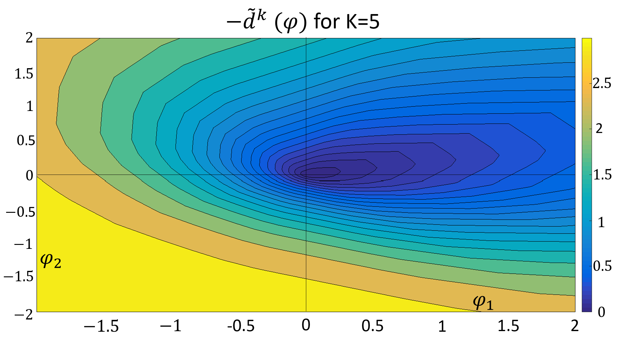
We illustrate the contour of for Example 4.8 in Figure 2.
As expected, the approximation of is best near (cf. Figure 1).
Figure 2: Contour levels for with for from
Example 4.8
In conclusion, Theorems 4.7 and 4.10 yield two ACRM stemming from expected down–trade log series
of (3.4) and its second approximation from (3.22). However, the first approximation
from (3.15) was not an ACRM since the coefficients in (3.16) are not continuous. At first glance,
however, this is puzzling: since is clearly continuous and equals for
sufficiently small according to Theorem 3.8, has to be continuous for small , too.
So what have we missed? In order to unveil that “mystery”, we give another representation for the expected down–trade log series
using again of (3.12)
Lemma 4.11.
In the situation of Theorem 3.8 for all and with the following holds:
(4.10)
Proof.
(4.10) can be derived from the definition in (3.4) as follows:
For with (3.7) clearly
holds. Introducing for the set
(4.11)
and using the characteristic function of a set , we obtain for all
Observe that has a similar representation, namely, using
(4.13)
we get right from the definition in (3.15) that for all
(4.14)
holds. So the only difference of (4.12) and (4.14) is that is replaced by (with the latter being a half–space restricted to ).
Observing furthermore that due to (3.21)
(4.15)
the discontinuity of clearly comes from the discontinuity of the indicator function , because
and the “mystery” is solved since Lemma 3.5(b)
implies equality in (4.15) for sufficiently small . Finally note that for large not only the
continuity gets lost, but moreover is no longer concave. The discontinuity can even be seen
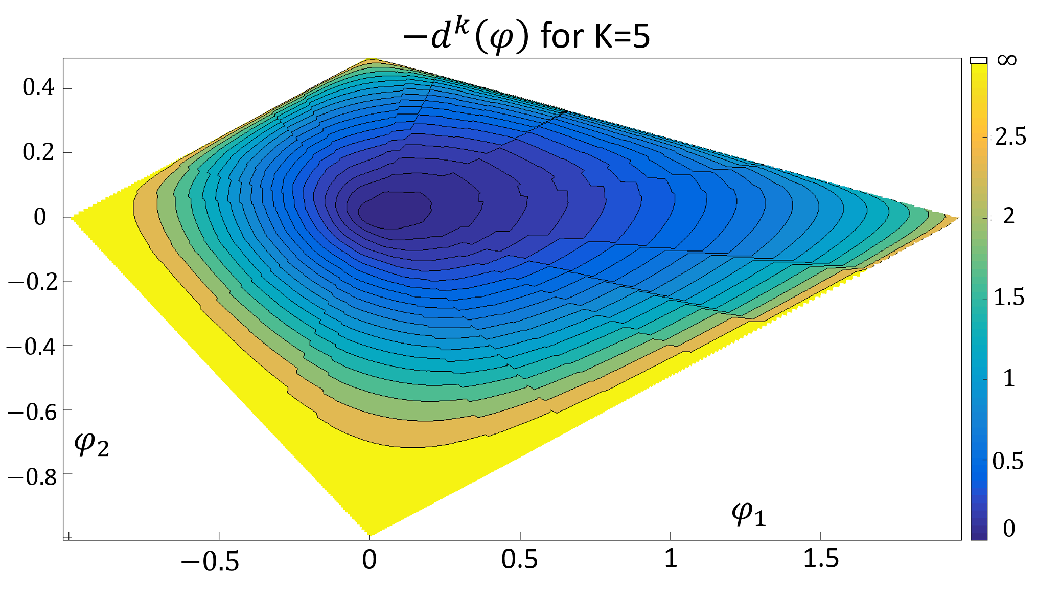
in Figure 3.
Figure 3: Discontinuous contour levels for with for from
Example 4.8
5 The current drawdown
We keep discussing the trading return matrix from (2.1) and probabilities from Setup 3.1 for each
row of . Drawing randomly and independently times such rows from that distribution results in a terminal wealth relative for
fractional trading
depending on the betted portions , see (3.1). In order to investigate the current drawdown
realized after the –th draw, we more generally use the notation
(5.1)
The idea here is that is viewed as a discrete “equity curve” at time (with and fixed).
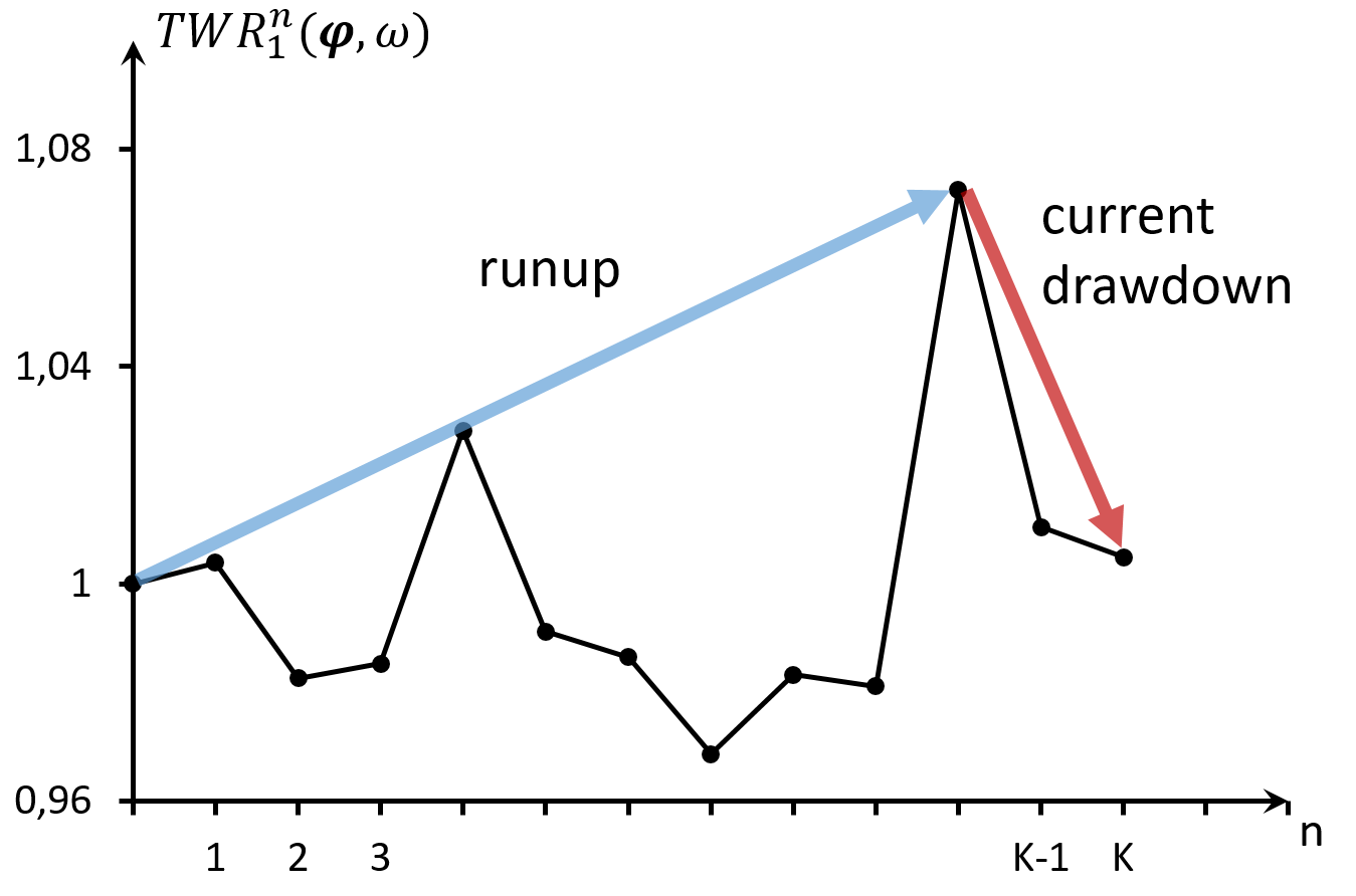
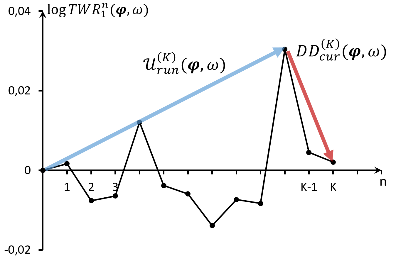
The current drawdown log series is defined as the logarithm of the drawdown of this equity curve realized from the maximum of the curve till
the end (time ). We will see below that this series is the counter part of the run–up (cf. Figure 4).
Figure 4: In the left figure the run-up and the current drawdown is plotted for a realization
of the TWR “equity”–curve and to the right are their log series.
Definition 5.1.
The current drawdown log series is set to
(5.2)
and the run-up log series is defined as
The corresponding trade series are connected because the current drawdown starts after the run–up has stopped.
To make that more precise, we fix that where the run–up reached its top.
Definition 5.2.
(first topping point)
For fixed and define with
(a)
in case
(b)
and otherwise choose such that
(5.3)
where should be minimal with that property.
By definition one easily gets
(5.4)
and
(5.5)
As in Section 3 we immediately obtain
and therefore by Theorem 3.2:
Corollary 5.3.
For
(5.6)
holds.
Explicit formulas for the expectation of and are again of interest.
By definition and with (5.4)
(5.7)
Before we proceed with this calculation we need to discuss further for some fixed .
By Definition 5.2, in case , we get
(5.8)
since is the first time the run-up topped, and, in case ,
(5.9)
Similarly as in Section 3 we again write as for and .
The last inequality then may be rephrased for and some sufficiently small as
(5.10)
by an argument similar as in Lemma 3.5. Analogously one finds for all
(5.11)
This observation will become crucial to proof the next result on the expectation of the current drawdown.
Theorem 5.4.
Let a trading game as in Setup 3.1 with be fixed.
Then for and the following holds:
(5.12)
where is independent of and for the functions
are defined by
(5.13)
Proof.
Again the proof is very similar as the proof in the univariate case, see Theorem 5.4 in [11].
Starting with (5.7) we get
holds, where is independent from and for the functions
are given as
(5.23)
Remark 5.7.
Again, we immediately obtain a first order approximation for the expected current drawdown log series. For
(5.24)
holds. Moreover, since
and holds as well.
As discussed in Section 4 for the down-trade log series, we also want to study the current drawdown log series
(5.2) with respect to admissible convex risk measures.
Theorem 5.8.
For a trading game as in Setup 3.1 satisfying Assumption 2.3 the
function
(5.25)
is an admissible convex risk measure (ACRM).
Proof.
It is easy to see that the proof of Theorem 4.7 can almost literally be adapted to the current drawdown case.
∎
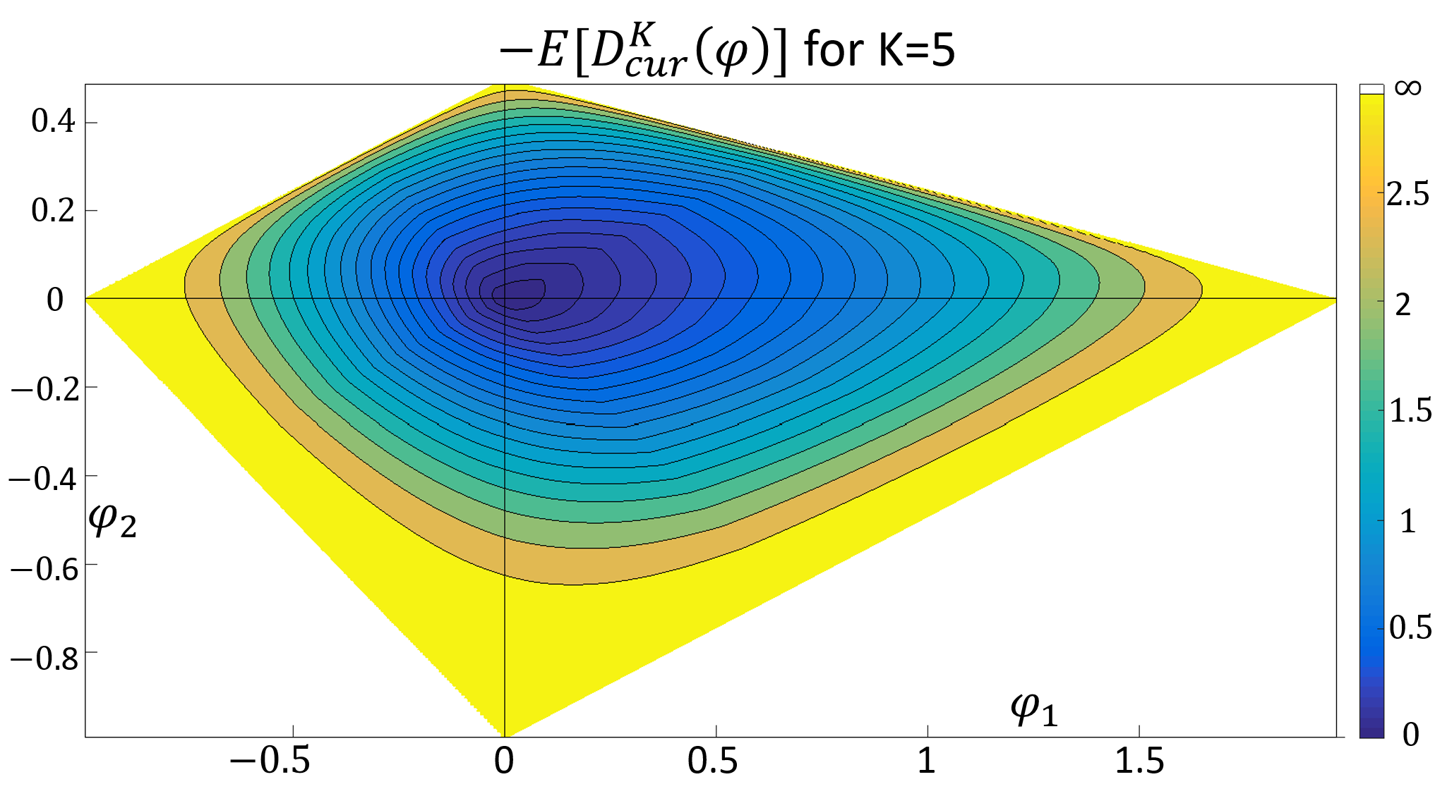
Figure 5: Contour levels for from (5.25) with for
Example 4.8
Confer Figure 5 for an illustration of . Compared to in
Figure 1 the contour plot looks quite similar, but near obviously grows faster.
Similarly, we obtain an ACRM for the first order approximation in (5.24):
Theorem 5.9.
For the trading game of Setup 3.1 satisfying Assumption 2.3 the function ,
with
(5.26)
is an admissible convex risk measure (ACRM) according to Definition 4.1 which is moreover positive homogeneous.
Proof.
We use (5.14) to derive the above formula for .
Now most of the arguments of the proof of Theorem 4.10 work here as well once we know that
is continuous in . To see that, we remark once more that for the first topping point
of the linearized equity curve
, the following holds
(cf. Definition 5.5 and (5.18)):
Thus
Although the topping point for may jump when is varied in case for some , i.e.
the continuity of is still granted since over all is summed. Hence, all claims are proved.
∎
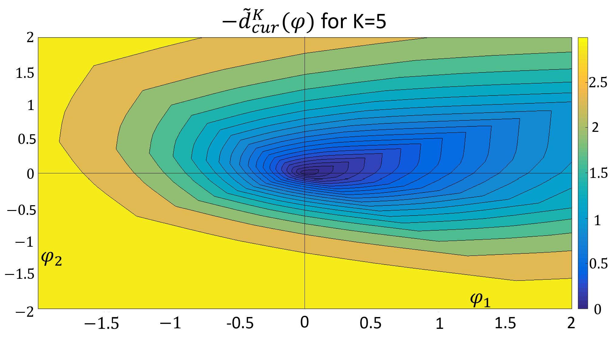
Figure 6: Contour levels for from Theorem 5.9 with for
Example 4.8
A contour plot of can be seen in Figure 6. The first topping point of the linearized equity
curve will also be helpful to order the risk measures and .
Reasoning as in (5.10) (see also Lemma 3.5) and using that (5.18) we obtain in case
for and that
(5.27)
However, since is concave, the above implication holds true even for all with . Hence for and
(5.28)
Looking at (5.9) once more, we observe that the first topping point of the equity curve necessarily is
less than or equal to . Thus we have shown:
The second inequality in (5.30) follows as in Section 3 from (see (5.12) and (5.24))
and the third inequality is already clear from Remark 5.7.
∎
6 Conclusion
Let us summarize the results of the last Sections. We obtained two down–trade log series related admissible convex risk measures (ACRM)
according to Definition 4.1, namely
see Corollary 3.12 and Theorems 4.7 and 4.10. Similarly we obtained two current drawdown related (ACRM),
namely
cf. Theorems 5.8 and 5.9 as well as Theorem 5.11.
Furthermore, due to Remark 5.7 we have the ordering
(6.1)
All four risk measures can be used in order to apply the general framework for portfolio theory of [12].
Since the two approximated risk measures and are positive homogeneous, according to [12],
the efficient portfolios will have an affine linear structure. Although we were able to prove a lot of results for these for practical applications
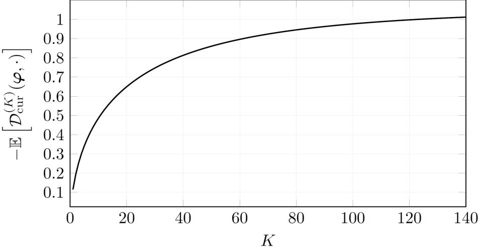
relevant risk measures, there are still open questions. To state only one of them, we note that convergence of these risk measures for is
unclear, but empirical evidence seems to support such a statement (see Figure 7).
Figure 7: Convergence of with fixed
for Example 4.8
Appendix A Transfer of a one–period financial market to the TWR setup
The aim of this appendix is to show that a one–period financial market can be transformed into the Terminal Wealth Relative (TWR)
setting of Ralph Vince [17] and [18]. In particular we show how the trade return matrix of
(2.1) has to be defined in order to apply the risk measure theory for current drawdowns of Section 4
and 5 to the general framework for portfolio theory of Maier-Paape and Zhu of Part I [12].
Setup A.1.
(one–period financial market) Let be a financial market in a one–period economy.
Here and represents a risk free bond, whereas the other components represent the price of the –th risky asset at time and is the vector
of all risky assets. is assumed to be a constant vector whose components are the prices of the assets at .
Furthermore is assumed to be a random vector on a finite probability space , i.e. represents the new price at for the risky assets.
Assumption A.2.
To avoid redundant risky assets, often the matrix
(A.1)
is assumed to have full rank , in particular .
A portfolio is a column vector whose components represent the investments in the –th asset, . In order to normalize that situation, we consider portfolios with unit initial cost, i.e.
(A.2)
Since this implies
(A.3)
Therefore the interpretation in Table 1 is obvious.
portion of capital invested in bond
portion of capital invested in –th risky asset,
Table 1: Invested capital portions
So if an investor has an initial capital of in his depot, the invested money in the depot is divided
as in Table 2.
cash position of the depot
invested money in –th asset,
amount of shares of –th asset to be bought at
Table 2: Invested money in depot for a portfolio
Clearly is the (random) gain of the unit initial cost portfolio
relative to the riskless bond. In such a situation the merit of a portfolio is often measured by its
expected utility , where is an increasing concave utility function
(see [12], Assumption 3.3).
In growth optimal portfolio theory the natural logarithm is used yielding the optimization problem
(A.6)
The following discussion aims to show that the above optimization problem (A.6) is an alternative way
of stating the Terminal Wealth Relative optimization problem of Vince (cf. [5], [16]).
Assuming all have the same probability (Laplace situation), i.e.
(A.7)
we furthermore get
(A.10)
This results in a “trade return” matrix
(A.11)
whose entries represent discounted relative returns of the –th asset for the –th reali-
zation . Furthermore,
the column vector with components has according to Table 1 the interpretation given in Table 3.
portion of capital invested in –th risky asset,
Table 3: Investment vector for the model
Thus we get
(A.14)
which involves the usual Terminal Wealth Relative () of Ralph Vince [16] and therefore under the assumption of a
Laplace situation (A.7) the optimization problem (A.6) is equivalent to
(A.15)
Furthermore, the trade return matrix in (A.11) may be used to define admissible convex risk measures as
introduced in Definition 4.1 which in turn give nontrivial applications to the general framework for
portfolio theory in Part I [12].
To see that, note again that by (A.10) any portfolio vector of a unit cost portfolio (A.2) is in one to one correspondence to an investment vector
(A.16)
for a diagonal matrix with only positive diagonal entries .
Then we obtain:
Theorem A.3.
Let be any of our four down–trade or drawdown related risk measures and (see (6.1))
for the trading game of Setup 3.1 satisfying Assumption 2.3.
Then
(A.17)
has the following properties:
(r1)
depends only on the risky part of the portfolio .
(r1n)
if and only if .
(r2)
is convex in .
(r3)
The two approximations and furthermore yield positive homogeneous , i.e.
for all .
Proof.
See the respective properties of (cf. Theorems 4.7, 4.10, 5.8 and 5.9).
In particular and are admissible convex risk measures according to Definition 4.1 and thus follow.
∎
Remark A.4.
It is clear that therefore or
can be evaluated on any set of admissible portfolios according to Definition 2.2 of [12] if
and the properties (r1), (r1n), (r2) (and only for and also (r3))
in
Assumption 3.1 of [12] follow from Theorem A.3.
In particular and satisfy the conditions of a deviation
measure in [14] (which is defined directly on the portfolio space).
Remark A.5.
Formally our drawdown or down–trade is a function of a TWR equity curve of a –period financial market.
But since this equity curve is obtained by drawing times stochastically independent from one and the
same market in Setup A.1, we still can work with a one–period market model.
We want to close this section with some remarks on the often used no arbitrage condition of the one–period financial market
and Assumption 2.3 which was necessary to construct admissible convex risk measures.
Definition A.6.
Let be a one–period financial market as in Setup A.1.
(a)
A portfolio is an arbitrage for if it satisfies
(A.18)
or, equivalently, if is satisfying
(A.19)
(b)
The market is said to have no arbitrage, if there exists no arbitrage portfolio.
Once we consider the above random variables as vector , (A.19) may equivalently be stated as
(A.20)
where we used the positive cone in .
Observe that the portfolio can never be an arbitrage portfolio.
Hence we get:
market has no arbitrage
(A.21)
(A.22)
where we used the negative cone in .
Note that the last equivalence leading to (A.22) follows, because with always also holds true.
According to Setup A.1, the matrix has full rank, and therefore for all anyway.
Hence we proceed
(A.26)
Observe that for all and the following is equivalent
(A.29)
Hence
(A.32)
(A.34)
using again the argument that also implies .
To conclude, (A.34) is exactly Assumption 2.3 and therefore we get:
Theorem A.7.
Let a one–period financial market as in Setup A.1 be given that satisfies Assumption A.2, i.e. from
(A.1) has full rank . Then the market has no arbitrage if and only if the in (A.10) and (A.11)
derived trade return matrix satisfies Assumption 2.3.
A very similar theorem is derived in [12].
For completeness we rephrase here that part which is important in the following.
Theorem A.8.
([12], Theorem 3.9) Let a one–period financial market as in Setup A.1 with no arbitrage be given. Then the conditions in Assumption 2.3
are satisfied for from (A.10) and (A.11) if and only if Assumption A.2 holds, i.e.
if from (A.1) has full rank .
Proof.
Note that the conditions in Assumption 2.3 for from (A.10) and (A.11)
are equivalent to
(A.37)
which follows directly from the equivalence of (A.34) and (A.26). But (A.37) is exactly the
point (ii*) in [12], Theorem 3.9, and Assumption A.2 is exactly the point (iii) of that theorem.
Therefore, under the no arbitrage assumption again by [1], Theorem 3.9, the claimed equivalence follows.
∎
Together with Theorem A.7 we immediately conclude:
Corollary A.9.
(two out of three imply the third)
Let a one–period financial market according to Setup A.1 be given. Then any two of the following conditions
imply the third:
(a)
Market has no arbitrage.
(b)
The trade return matrix from (A.10) and (A.11) satisfies Assumption 2.3.
(c)
Assumption A.2 holds, i.e. from (A.1) has full rank .
Remark A.10.
The standard assumption on the market in Part I [12] is “no nontrivial riskless portfolio”,
where a portfolio is riskless if
and is nontrivial if .
Using this notation we get:
Corollary A.11.
Consider a one–period financial market as in Setup A.1. Then there is no nontrivial riskless portfolio in if and
only if any two of the three statements (a), (b), and (c) from Corollary A.9 are satisfied.
Proof.
Just apply [12], Proposition 3.7 together with [12], Theorem 3.9 to the situation of
Corollary A.9.
∎
To conclude, any two of the three conditions of Corollary A.9 on the market are
sufficient to apply the theory presented in Part I [12].
References
[1]R. Brenner, S. Maier–Paape, A. Platen and Q.J. Zhu,A general framework for portfolio theory. Part III: applications,
in preparation.
[3]H. Föllmer and A. Schied,Stochastic Finance,
de Gruyter, (2002).
[4]A. Hermes,A Mathematical Approach to Fractional Trading, PhD–thesis,
Institut für Mathematik, RWTH Aachen, (2016).
DOI:
10.18154/RWTH-2016-11976
[5]A. Hermes and S. Maier–Paape,Existence and uniqueness for the multivariate discrete terminal wealth relative,
Risks, 5(3), 44, (2017).
DOI:
10.3390/risks5030044
[6]J. L. Kelly, Jr.,A new interpretation of information rate,
Bell System Technical J. 35:917-926, (1956).
DOI:
10.1002/j.1538-7305.1956.tb03809.x
[7]Marcos Lopez de Prado, Ralph Vince and Qiji Jim Zhu,Optimal risk budgeting under a finite investment horizon,
available at SSRN 2364092, (2013).
DOI:
10.2139/ssrn.2364092
[8]L.C. MacLean, E.O. Thorp and W.T. Ziemba,The Kelly Capital Growth Investment Criterion: Theory and Practice,
World Scientific, (2009).
[9]S. Maier–Paape,Existence theorems for optimal fractional trading,
Institut für Mathematik, RWTH Aachen, Report No. 67 (2013).
[10]S. Maier–Paape,Optimal and diversification,
International Federation of Technical Analysts Journal, ISSN 2409–0271, 15:4-7, (2015).
[11]S. Maier–Paape,Risk averse fractional trading using the current drawdown,
Institut für Mathematik, RWTH Aachen, Report No. 88 (2016).
https://arxiv.org/abs/1612.02985
[12]S. Maier–Paape and Q. J. Zhu,A general framework for portfolio theory. Part I: theory and various models,
Institut für Mathematik, RWTH Aachen, Report No. 91 (2017).
[13]H. M. Markowitz,Portfolio Selection,
Cowles Monograph, No. 16, Wiley, New York, (1959).
[14]R. T. Rockafellar, S. Uryasev and M. Zabarankin,Master funds in portfolio analysis with general deviation measures,
J. Banking and Finance, 30:743–778, (2006).
[15]W.F. Sharpe,Capital asset prices: A theory of market equilibrium under conditions of risk,
Journal of Finance, 19:425-442, (1964).
[16]R. Vince,The New Money Management: A Framework for Asset Allocation,
John Wiley & Sons, New York, (1995).
[17]R. Vince,The Mathematics of Money Management, Risk Analysis Techniques
for Traders,
A Wiley Finance Edition, John Wiley & Sons, New York, (1992).
[18]R. Vince,The Leverage Space Trading Model: Reconciling Portfolio Management
Strategies and Economic Theory,
John Wiley & Sons, Hoboken, NJ, (2009).
[19]R. Vince and Q.J. Zhu,Optimal betting sizes for the game of blackjack,
Risk Journals: Portfolio Management, 4:53-75, (2015)
[20]K. van Tharp,Van Tharp’s Definite Guide to Position Sizing,
The International Institute of Trading Mastery, Cary, NC, (2008).
[21]Q.J. Zhu,Mathematical analysis of investment systems,
J. Math. Anal. Appl. 326: 708–720, (2007).
[22]Q.J. Zhu,Convex analysis in mathematical finance,
Theory Method and Applications 75: 1719–1736, (2012).