Ultimate precision of joint quadrature parameter estimation with a Gaussian probe

Abstract

The Holevo Cramér-Rao bound is a lower bound on the sum of the mean-square error of estimates for parameters of a state. We provide a method for calculating the Holevo Cramér-Rao bound for estimation of quadrature mean parameters of a Gaussian state by formulating the problem as a semidefinite program. In this case, the bound is tight; it is attained by purely Guassian measurements. We consider the example of a symmetric two-mode squeezed thermal state undergoing an unknown displacement on one mode. We calculate the Holevo Cramér-Rao bound for joint estimation of the conjugate parameters for this displacement. The optimal measurement is different depending on whether the state is entangled or separable.

I Introduction

Quantum mechanics sets a limit on how accurately one can measure two noncommuting observables. This is exemplified by the Heisenberg uncertainty relation for position and momentum, which can be generalized to arbitrary observables Robertson (1929). This relation sets a precision limit to state estimation problem of the noncommuting observables. For example if we were to simultaneously measure two quadrature operators $\mathcal{Q}$ and $\mathcal{P}$ with the canonical commutation relation $[\mathcal{Q},\mathcal{P}]=i$ Weedbrook et al. (2012); Adesso et al. (2014) of a quantum state $\rho$, then the precision is limited by $\Delta{\mathcal{Q}}\Delta{\mathcal{P}}\geq\frac{1}{2}$. However if we are interested in estimating channel parameters instead, this restriction do not apply. In this case, entanglement can be used to enhance the precision of channel parameter estimates Giovannetti et al. (2004); D’Ariano et al. (2001); Fujiwara (2001); Fischer et al. (2001); Sasaki et al. (2002); Fujiwara and Imai (2003); Ballester (2004), for example, estimating the squeezing applied to a probe Rigovacca et al. (2017). Light-matter interferometry can be used to improve the estimate of a Gaussian process applied to a matter system Ruppert and Filip (2017). The precision can also be improved with a cleverly chosen single-mode state, for the estimation of a small displacement, for example Duivenvoorden et al. (2017).

We will consider in detail the example of estimation of the parameters $\theta_{1}$ and $\theta_{2}$ of the displacement operation

$$D(\theta_{1},\theta_{2})=\exp(i\theta_{2}\mathcal{Q}-i\theta_{1}\mathcal{P})\;,$$ (1)

acting on a probe state. It was shown in Refs.  D’Ariano et al. (2001); Genoni et al. (2013) that by using a two-mode entangled probe, one can estimate the displacement to arbitrary high accuracy. The probe is a symmetric two-mode squeezed thermal state. If the state is pure, it is known as a two-mode squeezed vacuum state, or an Einstein-Podolski-Rosen (EPR) state Weedbrook et al. (2012). By symmetric we mean that the state has equal squeezing and noise in all quadratures.

A measurement was proposed that can give an arbitrarily precise estimate of both $\theta_{1}$ and $\theta_{2}$ simultaneously. This measurement, which resembles continuous variable super-dense coding Braunstein and Kimble (2000), involves passing one mode on an entangled probe to sense the displacement operation and then jointly measuring it with an entangled ancilla. We call this measurement the double-homodyne joint measurement [see Fig. 1(b)]. This extremely precise estimation scheme was experimentally demonstrated in an optical system Li et al. (2002).

Genoni et al. Genoni et al. (2013) showed that for a symmetric two-mode squeezed state probe, in the limit of large entanglement, the double-homodyne joint measurement approaches the ultimate precision bounds calculated using the symmetric logarithmic derivative (SLD) quantum Fisher information. However, for a general finite squeezing level, there is a gap between the precision of the estimation from dual homodyne measurement and the limit set by the right logarithmic derivative (RLD) and SLD quantum Fisher information. This is not surprising since in general we know that the RLD and SLD bounds are not tight Szczykulska et al. (2016). This raises two questions: (i) Can we derive tight bounds for the precision? and (ii) Is there a better measurement that will give a higher precision than the dual homodyne measurement?

We address these questions for a general two-mode Gaussian probe. In this work, we calculate the Holevo Cramér -Rao (CR) bound Holevo (2011, 1976), which is an asymptotically achievable bound under some conditions Yamagata et al. (2013); Hayashi and Matsumoto (2008); Guţă and Kahn (2006); Kahn and Guţă (2009). However, unlike the RLD and SLD bounds, computing the Holevo bound is in general a hard problem because it involves an optimisation of a nonlinear function over a space of Hermitian matrices. To date, it has been solved in only a few simple cases. Providing the states satisfy certain conditions, an explicit formula can be found for Gaussian states Holevo (2011, 1975) or pure states Fujiwara and Nagaoka (1995); Matsumoto (2002). Suzuki found a formula in terms of the RLD and SLD CR bounds, for a qubit state parameterized by two parameters Suzuki (2016).

Previously, we performed this optimization for the special case when the probe was a pure two-mode entangled state, and one mode experiences an unknown displacement Bradshaw et al. (2017). When the probe is mixed or if the channel is dissipative, then the space of the optimisation problem is over infinite dimensional Hermitian matrices. However, for Gaussian states, the probe and measurement can be completely characterised by its first and second moment Holevo (2011, 1976). This reduces the optimisation space to four-dimensional positive semi-definite matrices which can be solved efficiently using semi-definite programming (SDP) Vandenberghe and Boyd (1996). Furthermore, the SDP and its dual program provide a necessary and sufficient condition for optimality of the solution, which can be verified analytically. Holevo solved the problem for mean estimation of Gaussian states 40 ago Holevo (2011, 1976). Our contribution is to recognise this as an SDP that can be solved efficiently.

For the specific case of a symmetric two-mode squeezed state, we find that the double-homodyne joint measurement is an optimal measurement when the squeezing level is high enough such that the probe is entangled. When the probe is separable, we find that the double-homodyne joint measurement is sub-optimal. We propose a different measurement scheme which is optimal.

In this paper, we provide a recipe for calculating the ultimate precision of an unbiased estimate of displacement using a two-mode Gaussian probe. We start with an introduction to multi-parameter local quantum estimation in Sec. II. In Sec. III, we formulate the problem of displacement estimation for two-mode Gaussian states in terms of an SDP. Section IV gives an application of this formalism to the symmetric two-mode squeezed state. Finally, we end with some concluding remarks in Sec. V.

II Multi-parameter local estimation

In classical parameter estimation theory, one starts with a random variable $X$ that depends on some unknown parameter vector $\theta=(\theta_{1},\theta_{2},\ldots,\theta_{N})$ through a conditional probability density function $f(x;\theta)$. The random variable $X$ arises from the measurement of some state $\rho(\theta$. From $X$, one can form a vector function $\hat{\theta}=\hat{\theta}(X)$ that gives an unbiased estimate of $\theta$. The goal is to find a precise estimate of theta. The bound on how precise these unbiased estimator can be is determined by the CR bound Cramér (2016); Rao (1992),

$$V_{\theta}[\hat{\theta}]\geq\frac{1}{I},$$ (2)

which relates the mean-square error (MSE) matrix

$$V_{\theta}[\hat{\theta}]_{jk}\coloneqq\mathbb{E}[(\hat{\theta}_{j}-\theta_{j})(\hat{\theta}_{k}-\theta_{k})]$$ (3)

to the classical Fisher information matrix

$$I_{jk}\coloneqq-\mathbb{E}\left[\frac{\partial^{2}}{\partial\theta_{j}\partial\theta_{k}}\log f\right]\;.$$ (4)

Under certain conditions, this bound can be asymptotically achieved by the maximum likelihood estimator. We are interested in the sum of the MSE, obtained by taking the trace of the MSE matrix $\Sigma\coloneqq\Tr{V_{\theta}[\hat{\theta}]}$.

Quantum parameter estimation theory Paris (2009); Helstrom (1969); Braunstein and Caves (1994); Braunstein et al. (1996) aims to determine the ultimate precision with which certain parameters $\theta$ can be determined from a quantum state $\rho_{\theta}$ that depends on those parameters. This was developed by Helstrom Helstrom (1969, 1967); Helstrom and Kennedy (1974), Holevo Holevo (2011, 1976) and others Yuen and Lax (1973); Belavkin (1976) in the 1970s. There exists a whole family of quantum Fisher information matrices, each of which gives rise to its own CR bounds to the mean-square error matrix Petz and Ghinea (2011). However, none of these bounds are generally tight. Two commonly used CR bounds are based on the SLD Helstrom (1967, 1969) and RLD Yuen and Lax (1973); Belavkin (1976) Fisher information matrix.

The SLD operators $L^{(\text{S})}_{j}$ and RLD operators $L^{(\text{R})}_{j}$ are obtained as solutions to the implicit operator equations

$$\frac{\partial\rho}{\partial\theta_{j}} =\frac{1}{2}\left(\rho L^{(\text{S})}_{j}+L^{(\text{S})}_{j}\rho\right)\;\text{(SLD)}$$ (5)

$$\frac{\partial\rho}{\partial\theta_{j}} =\rho L^{(\text{R})}_{j}\;\text{(RLD)}\;.$$ (6)

The SLD operators are Hermitian but the RLD operators might not be Hermitian. From the log-derivative operators, the SLD and RLD Fisher information matrices are defined by

$$G^{\text{(S)}}_{jk} \coloneqq\tr(\rho\frac{1}{2}(L^{(\text{S})}_{j}L^{(\text{S})}_{k}+L^{(\text{S})}_{k}L^{(\text{S})}_{j}))\;\text{(SLD)},$$ (7)

$$G^{\text{(R)}}_{jk} \coloneqq\tr(\rho L^{(\text{R})}_{j}L^{\text{(R)}\dagger}_{k})\;\text{(RLD)},$$ (8)

from which we get the two CR bounds

$$\Sigma \geq\Tr{(G^{(S)})^{-1}}\eqqcolon C^{\text{(S)}},$$ (9)

$$\Sigma \geq\Tr{\real(G^{(R)})^{-1}}+\text{TrAbs}\left\{\imaginary(G^{(R)})^{-1}\right\}\eqqcolon C^{\text{(R)}},$$ (10)

where $\text{TrAbs}\{X\}$ is the sum of the absolute values of the eigenvalues of a matrix $X$. The SLD CR bound, $C^{\text{(S)}}$ gives the optimal precision in estimating each parameter separately. However, for multi-parameter estimation, if optimal measurements for measuring each parameter separately do not commute (which is usually the case), then the SLD bound is not attainable. The RLD bound, $C^{\text{(R)}}$ is also in general not attainable. However, when $L^{(\text{R})}$ is Hermitian, $C^{\text{(R)}}$ provides an achievable bound for the joint estimates Fujiwara (1994a); Fujiwara and Nagaoka (1999); Fujiwara (1994b). In general, there is no hierarchy between $C^{\text{(S)}}$ and $C^{\text{(R)}}$.

Holevo unified these two bounds through the Holevo CR bound Holevo (2011, 1976). This bound is achieved in the asymptotic limit of a joint measurement over infinite copies of the state Yamagata et al. (2013). The Holevo CR bound is always greater or equal to $C^{\text{(S)}}$ and $C^{\text{(R)}}$. The bound involves a minimization over $X=(X_{1},X_{2},\ldots,X_{N})$ where $X_{j}$ are Hermitian operators that satisfy the unbiased conditions

$$\tr(\rho X_{j}) =0,$$ (11)

$$\tr(\frac{\partial\rho_{\theta}}{\partial\theta_{j}}X_{k}) =\delta_{jk}.$$ (12)

The Holevo CR bound is

$$\mathcal{V}\geq\min_{X}\text{Tr}\left\{Z_{\theta}[X]\right\}+\text{TrAbs}\left\{\imaginary Z_{\theta}[X]\right\}\coloneqq C^{\text{(H)}}\;,$$ (13)

where

$$Z_{\theta}[X]_{jk}\coloneqq\tr\left(\rho X_{j}X_{k}\right)\;.$$ (14)

Holevo derived this bound in his original work Holevo (2011, 1976), but the bound in this form was introduced by Nagaoka Nagaoka (2005). A major obstacle preventing the more widespread use of the Holevo CR bound is that unlike the RLD and SLD bounds, which can be calculated directly, the Holevo bound involves a nontrivial optimisation problem.

III Holevo bound for mean value estimation with Gaussian probes

When the probe is Gaussian, Holevo’s bound can be simplified. It can be formulated in terms of the first and second moments of the probe state only. In this section, we summarise Holevo’s result on mean value estimation of Gaussian probes. For the proofs and technicalities of these results, we recommend the interested reader to consult Holevo’s original work Holevo (2011, 1976).

III.1 Holevo’s bound

We want to estimate two parameters $\theta_{1}$ and $\theta_{2}$ that are imprinted on the displacement of a two-mode Gaussian state. Extension to more parameters or mode are straight forward (see Appendix C). To arrive at Holevo’s result we need to introduce some notations.

For any $z=\begin{bmatrix}y_{1}&x_{1}&y_{2}&x_{2}\end{bmatrix}^{\intercal}$ in a four-dimensional real vector space $Z$, let

$$\mathcal{R}(z)=x_{1}\mathcal{P}_{1}+y_{1}\mathcal{Q}_{1}+x_{2}\mathcal{P}_{2}+y_{2}\mathcal{Q}_{2}\;,$$ (15)

where $\mathcal{P}_{j}$ and $\mathcal{Q}_{j}$ are the usual quadrature operators for the $j$-th mode in quantum optics. $\mathcal{R}(z)$ are called canonical observables, and the canonical commutation relation becomes

$$[\mathcal{R}(z),\mathcal{R}(z^{\prime})]=i\Delta(z,z^{\prime})\;,$$ (16)

where

$$\Delta(z,z^{\prime})=x^{\prime}_{1}y_{1}-x_{1}y^{\prime}_{1}+x^{\prime}_{2}y_{2}-x_{2}y^{\prime}_{2}$$ (17)

is a skew-symmetric bilinear form. By the Baker-Campbell-Hausdorff formula, we have an equivalent representation of the canonical commutation relation as

$$\mathcal{V}(z)\mathcal{V}(z^{\prime})=\exp\left(\frac{i}{2}\Delta(z,z^{\prime})\right)\mathcal{V}(z+z^{\prime})\;,$$ (18)

where $\mathcal{V}(z)=\mathrm{e}^{i\,\mathcal{R}(z)}$ is the Weyl operator. The characteristic function of a state $\mathcal{S}$ is then defined through $\mathcal{V}(z)$ as $\chi_{z}[\mathcal{S}]=\tr{\mathcal{S}\mathcal{V}(z)}$. This is the inverse-Weyl or Wigner transform that maps an operator in the Hilbert space to some square-integrable function in $Z$. We say $\mathcal{S}$ is Gaussian if the state is completely characterized by its first and second moments Weedbrook et al. (2012):

$$\chi_{z}[\mathcal{S}]=\exp\left[i\,m(z)-\frac{1}{2}\alpha(z,z)\right]\;,$$ (19)

where

$$m(z) =\tr(\mathcal{S}\mathcal{R}(z))$$ (20)

$$\alpha(z,z^{\prime}) =\frac{1}{2}\tr(\mathcal{S}\{\mathcal{R}(z)-m(z),\mathcal{R}(z^{\prime})-m(z^{\prime})\})\;$$ (21)

and $\{\mathcal{A},\mathcal{B}\}=\mathcal{A}\mathcal{B}+\mathcal{B}\mathcal{A}$. The mean value function $m$ is a function of the unknown parameters through

$$m(z)=\theta_{1}m_{1}(z)+\theta_{2}m_{2}(z)\;.$$ (22)

The correlation function $\alpha$ is an inner product on $Z$, which defines a Euclidean space $(Z,\alpha)$. Now let $\mathcal{D}$ be the associated operator of the form $\Delta$ in $(Z,\alpha)$,

$$\Delta(z,z^{\prime})=\alpha(z,\mathcal{D}z^{\prime})\;\forall\;z,z^{\prime}\in Z\;.$$ (23)

Define $m_{j}\in Z$ by $m_{j}(z)=\alpha(m_{j},z)$.

Holevo’s CR bound is

$$\Sigma\geq\inf_{\mathscr{F}}{\Tr{F^{-1}}}\eqqcolon\Sigma_{*}$$ (24)

where $F$ is a $2\times 2$ matrix with components

$$F_{jk}=\alpha(m_{j},\mathscr{F}m_{k})$$ (25)

and the infimum is taken over all real symmetric operators $\mathscr{F}$ in $Z$, such that the complex extension of $\mathscr{F}$ satisfies

$$0\leq(1+\tfrac{1}{2}i\mathcal{D})\mathscr{F}(1+\tfrac{1}{2}i\mathcal{D})\leq(1+\tfrac{1}{2}i\mathcal{D})$$ (26)

in the complexification of the Euclidean space $(Z,\alpha)$. $\mathcal{A}\leq\mathcal{B}$ denotes $\alpha(z,\mathcal{A}z)\leq\alpha(z,\mathcal{B}z)$ for all $z\in Z$. Since $1+\frac{1}{2}i\mathcal{D}$ is positive definite, constraint (26) is equivalent to

$$0\leq\mathscr{F}\leq(1+\tfrac{1}{2}i\mathcal{D})^{-1}.$$ (27)

III.2 Optimal measurement

For estimating the mean of Gaussian probes, Holevo showed that the bound can be attained by a Gaussian measurement. Let $\mathscr{F}_{*}$ be the operator in $Z$ that furnishes the minimum in (24) and $F_{*}$ be the corresponding matrix in (25). The optimal estimator are given by the observables $\mathcal{R}(z_{j}^{*})$ where

$$\begin{bmatrix}z_{1}^{*}\\ z_{2}^{*}\end{bmatrix}=F^{-1}_{*}\begin{bmatrix}\mathscr{F}_{*}m_{1}\\ \mathscr{F}_{*}m_{2}\end{bmatrix}\;.$$ (28)

$\mathcal{R}(z_{1}^{*})$ and $\mathcal{R}(z_{2}^{*})$ can be measured simultaneously to attain precision $\Sigma_{*}$.

III.3 Matrix representation

The optimisation problem for computing Holevo’s bound can be expressed as a semi-definite program. This can be clearly seen if we introduce four vectors $\{e_{1},e_{2},e_{3},e_{4}\}$ that forms an orthonormal basis in the Euclidean space $(Z,\alpha)$ such that $\alpha(e_{j},e_{k})=\delta_{jk}$ and introduce

$$\mathbb{D}_{jk} \coloneqq\alpha(e_{j},\mathcal{D}e_{k})\;$$ (29)

and

$$\mathbb{M}_{jk} \coloneqq\alpha(m_{j},e_{k}),$$ (30)

$$\mathbb{F}_{jk} \coloneqq\alpha(e_{j},\mathscr{F}e_{k}),$$ (31)

so that

$$F_{jk} =\alpha(m_{j},\mathscr{F}m_{k})$$ (32)

$$=\sum_{mn}\alpha(m_{j},e_{m})\,\alpha(e_{m},\mathscr{F}e_{n})\,\alpha(e_{n},m_{k})$$ (33)

$$=\left(\mathbb{M}\mathbb{F}\mathbb{M}^{\intercal}\right)_{jk}\;$$ (34)

Let $\mathbb{S}^{n}$ be the set of all $n\times n$ real symmetric matrices. Holevo’s bound is obtained as a solution to the following program:

Program 1

Holevo’s bound

$$\Sigma_{*}= \min_{\mathbb{F}\in\mathbb{S}^{4}}\Tr{F^{-1}}$$ (35)

subject to $$0\leq\mathbb{F}\leq\mathbb{C}\;,$$ (36)

where $F=\mathbb{M}\mathbb{F}\mathbb{M}^{\intercal}$ and $\mathbb{C}\coloneqq(1+\tfrac{1}{2}i\mathbb{D})^{-1}$. This is recognised as an SDP (see Appendix A) that can be solved efficiently using standard numerical techniques.

IV Worked example: Symmetric two-mode squeezed state

We illustrate the computation of Holevo’s bound through a specific example. We start with a mixed two-mode squeezed state $\rho_{0}=S_{2}(r)(\rho_{\text{th}}(v)\otimes\rho_{\text{th}}(v))S_{2}^{\dagger}(r)$ as our probe where

$$\rho_{\text{th}}(v)=\frac{2}{(1+2v)}\sum_{n}\left(\frac{2v-1}{2v+1}\right)^{n}\ket{n}\bra{n}$$ (37)

is a thermal state with mean photon number $v-\frac{1}{2}$ and quadrature variance $\alpha(z,z)=v$. The vacuum state corresponds to $v=\frac{1}{2}$. The ket $\ket{n}$ is the Fock state with $n$ photons, and

$$S_{2}(r)\coloneqq\exp\left(ra_{1}a_{2}-ra_{1}^{\dagger}a_{2}^{\dagger}\right)$$ (38)

is the two-mode squeezing operator where $a_{j}$ and $a_{j}^{\dagger}$ are the $j$-th mode annihilation and creation operators with commutation relation $[a,a^{\dagger}]=1$. Having prepared the probe $\rho_{0}$, we send one mode through a displacement

$$D(\theta_{1},\theta_{2})\coloneqq\exp\left(i\theta_{2}\mathcal{Q}_{1}-i\theta_{1}\mathcal{P}_{1}\right)$$ (39)

to get $\rho_{\theta}$, where $\theta_{1}$ and $\theta_{2}$ are the two unknown parameters that we wish to determine. In what follows, we shall compute the Holevo bound and present a measurement that achieves this bound. We then compare this bound with the RLD and SLD bounds.

IV.1 Problem formulation

Having the state $\rho_{\theta}$, we can already write its characteristic function and find Holevo’s bound directly. But, instead, we choose to perform a unitary transformation to decouple the two modes of the probe. The transformation we perform is

$$U=\exp\left(\frac{\pi}{4}(a_{1}^{\dagger}a_{2}-a_{1}a_{2}^{\dagger})\right),$$ (40)

which corresponds to interfering the two modes on a 50:50 beam splitter. This extra step is not necessary but is done for convenience so that the intermediate expressions in computing the bound become less cumbersome. This of course will not change the final result since the unitary operation can be considered part of the measurement. The correlation function is

$$\alpha(z,z^{\prime})=v\begin{bmatrix}y_{1}\\ x_{1}\\ y_{2}\\ x_{2}\end{bmatrix}^{\intercal}\begin{bmatrix}\mathrm{e}^{-2r}&0&0&0\\ 0&\mathrm{e}^{2r}&0&0\\ 0&0&\mathrm{e}^{2r}&0\\ 0&0&0&\mathrm{e}^{-2r}\end{bmatrix}\begin{bmatrix}y^{\prime}_{1}\\ x^{\prime}_{1}\\ y^{\prime}_{2}\\ x^{\prime}_{2}\end{bmatrix}$$ (41)

and mean

$$m(z)=\frac{1}{\sqrt{2}}\begin{bmatrix}\theta_{1}\\ \theta_{2}\\ -\theta_{1}\\ -\theta_{2}\end{bmatrix}^{\intercal}\begin{bmatrix}y_{1}\\ x_{1}\\ y_{2}\\ x_{2}\end{bmatrix}\;.$$ (42)

From this, the two vectors $m_{1}$ and $m_{2}$ in $Z$ are

$$m_{1} =\frac{1}{v\sqrt{2}}\begin{bmatrix}\mathrm{e}^{2r}&0&-\mathrm{e}^{-2r}&0\end{bmatrix}^{\intercal},$$ (43)

$$m_{2} =\frac{1}{v\sqrt{2}}\begin{bmatrix}0&\mathrm{e}^{-2r}&0&-\mathrm{e}^{2r}\end{bmatrix}^{\intercal}\;.$$ (44)

We now pick four orthonormal bases in $(\alpha,Z)$. Holevo’s bound does not depend on our choice of basis, any basis would do, and one such basis is:

$$\begin{bmatrix}e_{1}&e_{2}&e_{3}&e_{4}\end{bmatrix}=\frac{1}{\sqrt{v}}\begin{bmatrix}\mathrm{e}^{r}&0&0&0\\ 0&\mathrm{e}^{-r}&0&0\\ 0&0&\mathrm{e}^{-r}&0\\ 0&0&0&\mathrm{e}^{r}\end{bmatrix}\;.$$ (45)

In this basis,

$$\mathbb{M}=\frac{1}{\sqrt{2v}}\begin{bmatrix}\mathrm{e}^{r}&0&-e^{-r}&0\\ 0&\mathrm{e}^{-r}&0&-e^{r}\end{bmatrix}$$ (46)

and

$$\mathbb{D}=\frac{1}{v}\begin{bmatrix}0&1&0&0\\ -1&0&0&0\\ 0&0&0&1\\ 0&0&-1&0\end{bmatrix}.$$ (47)

We show in Appendix B that the solution to the SDP program (35) is

$$\Sigma_{*}=\begin{cases}\frac{4v^{2}-1}{2v\cosh 2r-1}&\text{if }r<r_{0}\\ 4v\mathrm{e}^{-2r}&\text{if }r\geq r_{0}\end{cases}$$ (48)

where $r_{0}=\frac{1}{2}\log(2v)$ and an optimal $\mathbb{F}_{*}$ attaining this is

$$\mathbb{F}_{*} =\frac{2v}{4v^{2}-1}\begin{bmatrix}2v-\mathrm{e}^{-2r}&0&0&0\\ 0&2v-\mathrm{e}^{2r}&0&0\\ 0&0&2v-\mathrm{e}^{2r}&0\\ 0&0&0&2v-\mathrm{e}^{-2r}\end{bmatrix}$$

for $r<r_{0}$ and

$$\mathbb{F}_{*} =\begin{bmatrix}1&0&0&0\\ 0&0&0&0\\ 0&0&0&0\\ 0&0&0&1\end{bmatrix}$$ (49)

for $r\geq r_{0}$.

IV.2 Optimal measurements that attains the bound

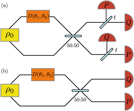
Figure 1: The probe state $\rho_{0}$, a two-mode squeezed state, undergoes an unknown displacement $D(\theta_{1},\theta_{2})$. This figure shows the optimal measurement for estimating the displacement. (a) The optimal measurement to perform when $r<r_{0}$ is a double-unbalanced-heterodyne joint measurement. The two modes a mixed with a 50:50 beam splitter. Each output of the beam splitter then passes through another beam splitter with transmission $t$ given by (52). Homodyne measurements of the $\mathcal{P}$ and $\mathcal{Q}$ quadratures are performed on the outputs of the beam splitters. (b) The optimal measurement to perform when $r\geq r_{0}$ is a double-homodyne joint measurement. The two modes are mixed with a 50:50 beam splitter. A homodyne measurement of the $\mathcal{P}$ quadrature is performed on one output of the beam splitter, and a homodyne measurement of the $\mathcal{Q}$ quadrature is performed on the other.

To find the optimal measurement achieving $\Sigma_{*}$, we substitute the solution for $\mathbb{F}_{*}$ into (28) to obtain $z_{j}^{*}$. For $r<r_{0}$

$$z_{1}^{*} =\sqrt{2}\begin{bmatrix}t&0&t-1&0\end{bmatrix}^{\intercal},$$ (50)

$$z_{2}^{*} =\sqrt{2}\begin{bmatrix}0&1-t&0&-t\end{bmatrix}^{\intercal},$$ (51)

where

$$t=\frac{2ve^{2r}-1}{4v\cosh 2r-2}.$$ (52)

The observable corresponding to this is

$$\begin{split}\mathcal{R}(z_{1}^{*})&=\sqrt{2}t\mathcal{Q}_{1}-\sqrt{2}(1-t)\mathcal{Q}_{2},\\ \mathcal{R}(z_{2}^{*})&=\sqrt{2}(1-t)\mathcal{P}_{1}-\sqrt{2}t\mathcal{P}_{2}\;,\end{split}$$ (53)

whose physical realisation is shown in Fig. 1(a).

For $r\geq r_{0}$, we have

$$z_{1}^{*} =\sqrt{2}\begin{bmatrix}1&0&0&0\end{bmatrix}^{\intercal},$$ (54)

$$z_{2}^{*} =\sqrt{2}\begin{bmatrix}0&0&0&-1\end{bmatrix}^{\intercal}\;,$$ (55)

which is a special case of Eq. (53) with $t=1$. The observables corresponding to these vectors are then

$$\mathcal{R}(z_{1}^{*}) =\sqrt{2}\mathcal{Q}_{1},$$ (56)

$$\mathcal{R}(z_{2}^{*}) =-\sqrt{2}\mathcal{P}_{2},$$ (57)

which is realized by the setup in Fig. 1(b). The two vectors $z_{1}^{*}$ and $z_{2}^{*}$ provide an unbiased estimator as can be checked by noticing that $m(z_{j}^{*})=\tr(\rho\mathcal{R}(z_{j}^{*}))=\theta_{j}$.

IV.3 Discussions

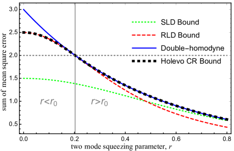
Figure 2: Plot of symmetric logarithmic derivative (SLD), right logarithmic derivative (RLD), and Holevo Cramér -Rao (CR) bounds, and double-homodyne joint measurement sum of mean-square error (MSE) for $v=0.75$. The vertical line corresponds to $r_{0}$. For $r\geq r_{0}$, the Holevo CR bound is equal to the sum of MSE of the double-homodyne joint measurement. For $r\leq r_{0}$, the Holevo CR bound is equal to the RLD bound and the sum of MSE for the double-unbalanced-heterodyne joint measurement. The horizontal line corresponds to the best sum of MSE when using a single-mode Gaussian probe.

Figure 2 shows the SLD and RLD CR bounds from Refs. Genoni et al. (2013); Gao and Lee (2014), our Holevo CR bound Eq. (48), and the sum of MSE for a double-homodyne joint measurement. The Holevo CR bound is greater than or equal to the RLD and SLD CR bounds. When $r\geq r_{0}$, the sum of MSE for the double-homodyne joint measurement is equal to the Holevo CR bound. When $r\leq r_{0}$, the Holevo CR bound is equal to the RLD CR bound. The double-unbalanced-heterodyne joint measurement outperforms the double-homodyne joint measurement in this case, giving a sum of MSE equal to the RLD and Holevo CR bounds. When $r>r_{0}$, the double-unbalanced-heterodyne joint measurement is impossible, requiring a beam splitter transmission greater than 1 [from Eq. (52)].

Interestingly, we note that $r_{0}$ is the threshold beyond which the probe becomes entangled as can be checked using Duan’s inseparability criterion Duan et al. (2000). At $r=r_{0}$, the sum of MSE is exactly $2$, which turns out to be the same as one get by doing a heterodyne measurement on a single-mode coherent state probe. This is the best one can do when restricted to single-mode Gaussian probes. Regardless of whether the probe is entangled or not, the optimal measurement scheme requires mixing the two modes on a 50:50 beam splitter, after which we end up with two uncorrelated states. If the probe state was originally entangled, the states after the 50:50 beam splitter will have a quadrature variance below the vacuum noise, while if the original state is separable, all quadrature variances will always be greater than the vacuum noise.

The double-unbalanced-heterodyne measurement can be seen as obtaining two independent estimates for each displacement parameter and then making an optimal estimate from these. As $t$ varies, the precision of one estimate decreases at the expense of a better precision for the second estimate. Suppose the system is entirely classical, and we have a classical state with covariances of $\mathcal{P}$ and $\mathcal{Q}$ the same as the quantum state. Because the system is classical, $\mathcal{P}$ and $\mathcal{Q}$ can be measured simultaneously without an additional noise penalty imposed by quantum mechanics. In this case, the double-unbalanced-heterodyne would outperform the dual-homodyne measurement as we get two independent estimates for $\theta_{1}$ and two independent estimates for $\theta_{2}$. However, for the quantum system, the double-unbalanced-heterodyne measurement incurs a noise penalty due to the vacuum noise coupling through the unused ports of the beam splitters. There is a trade-off between a decreased precision due to the vacuum noise, and an increased precision obtained from the availability of an independent second estimate. When the measurement noise is greater than the vacuum noise, the increase in precision we get from the second estimate outweighs the loss of precision due to the vacuum noise contaminating the first estimate. This is no longer true when the measurement noise is smaller than the vacuum noise.

Even when the probe is separable, the optimal measurement still requires a joint measurement of the two modes. Hence, perhaps counter-intuitively, the optimal measurement is not separable despite the probe being separable. Nevertheless, this is consistent with previous work Gu et al. (2012), where a joint measurement was found to provide a higher mutual information than a separable measurement. The performance advantage is attributed to the state having a nonzero quantum discord, despite having no entanglement.

V Conclusion

In conclusion, we provided a method to calculate the Holevo CR bound for the estimation of the mean quadrature parameters of a two-mode Gaussian state, by converting a problem to an SDP. An SDP can be efficiently solved numerically. Additionally, conditions proving optimality of an SDP solution exist, allowing for an analytical solution to be verified. Our method can be easily extended to Gaussian states with any number of modes.

Using this method we were able to find an analytical solution for the Holevo CR bound of the displacement on one mode of a symmetric two-mode squeezed thermal state. A double-homodyne joint measurement is optimal if the state is entangled, and a double-unbalanced-heterodyne joint measurement is optimal if the state is separable.

Appendix A Conversion of problem to semi-definite program (SDP)

We show that the problem of computing Holevo’s bound for mean value estimation of Gaussian states is a semi-definite program. We formulate the original problem of finding $\Sigma_{*}$ into a dual form SDP. Holevo’s bound is the following:

Program 2

Holevo’s bound

$$\Sigma_{*}= \min_{\mathbb{F}\in\mathbb{S}^{4}}\Tr{F^{-1}}$$ (58)

subject to $$0\leq\mathbb{F}\leq\mathbb{C}\;,$$ (59)

where $\mathbb{S}^{n}$ is the set of $n\times n$ real symmetric matrices, $F=\mathbb{M}\mathbb{F}\mathbb{M}^{\dagger}$, and $\mathbb{M}$ is a fixed real 2-by-4 matrix. Also $\mathbb{C}\coloneqq(1+\tfrac{1}{2}i\mathbb{D})^{-1}$ is a fixed Hermitian 4-by-4 matrix. To cast this nonlinear optimisation problem to an SDP, we use the standard trick of introducing an auxiliary 2-by-2 real matrix $H$ that serves as an upper bound to $F^{-1}$. So Holevo’s bound becomes

Program 3

$$\Sigma_{*}= \min_{\mathbb{F}\in\mathbb{S}^{4},H\in\mathbb{S}^{2}}\Tr{H}$$ (60)

subject to $$0\leq\mathbb{F}\leq\mathbb{C}$$ (61)

$$H\geq F^{-1}\;.$$ (62)

Consider

$$W(\mathbb{F},H)=\begin{bmatrix}H&I_{2}\\ I_{2}&F\end{bmatrix}\geq 0\$$ (63)

$$\Leftrightarrow W/F=H-F^{-1}\geq 0$$ (64)

$$\Leftrightarrow H\geq F^{-1},$$ (65)

where $W/F$ is the Schur’s complement of $F$ in $W$, and $I_{n}$ is the $n\times n$ identity matrix. We can formulate the SDP for $\Sigma_{*}$ as:

$$\Sigma_{*}=\min_{\mathbb{F}\in\mathbb{S}^{4},H\in\mathbb{S}^{2}}{\Tr{H}}$$ (66)

subject to

$$\begin{bmatrix}H&I_{2}\\ I_{2}&\mathbb{M}\mathbb{F}\mathbb{M}^{\dagger}\end{bmatrix}\oplus\mathbb{F}\oplus-\mathbb{F} \geq 0_{4}\oplus 0_{4}\oplus-\mathbb{C}$$ (67)

$$\Leftrightarrow\underbrace{\begin{bmatrix}H&0_{2}\\ 0_{2}&\mathbb{M}\mathbb{F}\mathbb{M}^{\dagger}\end{bmatrix}\oplus\mathbb{F}\oplus-\mathbb{F}}_{\sum_{j}y_{j}B_{j}} \geq\underbrace{\begin{bmatrix}0_{2}&-I_{2}\\ -I_{2}&0_{2}\end{bmatrix}\oplus 0_{4}\oplus-\mathbb{C}}_{C}\;,$$ (68)

where $0_{n}$ is the $n\times n$ zero matrix. We can decompose the LHS into a sum $\sum_{j}y_{j}B_{j}$ where $y=\begin{bmatrix}y_{1}&\ldots&y_{13}\end{bmatrix}^{\intercal}$ is a vector of real numbers and $B_{j}$ are the 13 matrices given by:

$$B_{j} =\begin{bmatrix}\mathbb{B}_{j}&0_{2}\\ 0_{2}&\mathbb{M}\mathbb{A}_{j}\mathbb{M}^{\dagger}\end{bmatrix}\oplus\mathbb{A}_{j}\oplus-\mathbb{A}_{j}\text{ for }j=1,\ldots,13\;.$$ (69)

$\{\mathbb{A}_{j}\}$ are 10 real symmetric matrices that forms a basis for the set of $4\times 4$ real symmetric matrices. Similarly, $\{\mathbb{B}_{j}\}$ are three real symmetric matrices that forms a basis for the set of $2\times 2$ real symmetric matrices. They are given by the following:

$$\mathbb{A}_{1} =\begin{bmatrix}1&0&0&0\\ 0&0&0&0\\ 0&0&0&0\\ 0&0&0&0\end{bmatrix} \quad\mathbb{A}_{2} =\begin{bmatrix}0&0&0&0\\ 0&1&0&0\\ 0&0&0&0\\ 0&0&0&0\end{bmatrix} \quad\mathbb{A}_{3} =\begin{bmatrix}0&0&0&0\\ 0&0&0&0\\ 0&0&1&0\\ 0&0&0&0\end{bmatrix} \quad\mathbb{A}_{4} =\begin{bmatrix}0&0&0&0\\ 0&0&0&0\\ 0&0&0&0\\ 0&0&0&1\end{bmatrix} \quad\mathbb{A}_{5} =\begin{bmatrix}0&1&0&0\\ 1&0&0&0\\ 0&0&0&0\\ 0&0&0&0\end{bmatrix}$$

$$\mathbb{A}_{6} =\begin{bmatrix}0&0&1&0\\ 0&0&0&0\\ 1&0&0&0\\ 0&0&0&0\end{bmatrix} \mathbb{A}_{7} =\begin{bmatrix}0&0&0&1\\ 0&0&0&0\\ 0&0&0&0\\ 1&0&0&0\end{bmatrix} \mathbb{A}_{8} =\begin{bmatrix}0&0&0&0\\ 0&0&1&0\\ 0&1&0&0\\ 0&0&0&0\end{bmatrix} \mathbb{A}_{9} =\begin{bmatrix}0&0&0&0\\ 0&0&0&1\\ 0&0&0&0\\ 0&1&0&0\end{bmatrix} \mathbb{A}_{10} =\begin{bmatrix}0&0&0&0\\ 0&0&0&0\\ 0&0&0&1\\ 0&0&1&0\end{bmatrix}$$

and $\mathbb{A}_{j}=0$ for $j=11,12,13$;

$$\mathbb{B}_{11}=\begin{bmatrix}1&0\\ 0&0\end{bmatrix}\quad\mathbb{B}_{12}=\begin{bmatrix}0&0\\ 0&1\end{bmatrix}\quad\mathbb{B}_{13}=\begin{bmatrix}0&1\\ 1&0\end{bmatrix}\quad\mathbb{B}_{j}=0\;\textrm{ for }j=1,\ldots,10\;.$$ (70)

The objective function can be written as $\tr{H}=y^{\intercal}\,b$ where $b=\setcounter{MaxMatrixCols}{13}\begin{bmatrix}0&0&0&0&0&0&0&0&0&0&1&1&0\end{bmatrix}^{\intercal}$. Finally, we have the problem statement as the following:

Program 4

Standard SDP dual problem formulation of Holevo’s bound

$$\Sigma_{*} =\min_{y}y^{\intercal}\,b$$ (71)

subject to $$\sum_{j}y_{j}B_{j}\geq C\;.$$ (72)

This is traditionally called the dual problem.

The primal problem statement is:

Program 5

Standard SDP primal problem formulation of Holevo’s bound

$$\Sigma^{*} =\max_{X}\Tr{CX}$$ (73)

subject to $$\Tr{B_{j}X}=b_{j}\textnormal{ for }j=1,\ldots,13,$$ (74)

where $X$ is a positive Hermitian matrix. This problem is bounded above and strictly feasible, which means that it satisfies strong duality: $\Sigma_{*}=\Sigma^{*}$.

Appendix B Solution to the worked example

In this appendix we provide the solution to the worked example. We present $X^{*}$ and $y^{*}$ that we claim is optimal. We first verify that $X^{*}$ and $y^{*}$ satisfy the primal and dual constraint. Next we show that the primal and dual value they provide are the same, indicating that the solution is optimal.

We consider the solutions for $r\geq r_{0}$ and $r<r_{0}$ separately.

B.1 Solution for $r<r_{0}$

For $r<r_{0}$, we claim that a solution is achieved by $y^{*}$ and $X^{*}$ having the form

$$y^{*} =\setcounter{MaxMatrixCols}{13}\begin{bmatrix}c_{1}&c_{2}&c_{2}&c_{1}&0&-c_{0}&0&0&-c_{0}&0&\frac{4v^{2}-1}{4v\cosh 2r-2}&\frac{4v^{2}-1}{4v\cosh 2r-2}&0\end{bmatrix}^{\intercal},$$ (75)

$$X^{*} =X_{1}^{*}\oplus 0_{4}\oplus X_{3}^{*},$$ (76)

where we are free to choose $c_{0}:$ $0\leq c_{0}\leq\frac{2v}{1-4v^{2}}+\frac{v}{2v\cosh 2r-1}$ and

$$c_{1} =\frac{2v(2v-\mathrm{e}^{-2r})}{4v^{2}-1}-\mathrm{e}^{-2r}c_{0},$$ (77)

$$c_{2} =\frac{2v(2v-\mathrm{e}^{2r})}{4v^{2}-1}-\mathrm{e}^{2r}c_{0},$$ (78)

$$X_{1}^{*} =\begin{bmatrix}1&0&-\frac{4v^{2}-1}{4v\cosh 2r-2}&0\\ 0&1&0&-\frac{4v^{2}-1}{4v\cosh 2r-2}\\ -\frac{4v^{2}-1}{4v\cosh 2r-2}&0&\frac{(4v^{2}-1)^{2}}{(4v\cosh 2r-2)^{2}}&0\\ 0&-\frac{4v^{2}-1}{4v\cosh 2r-2}&0&\frac{(4v^{2}-1)^{2}}{(4v\cosh 2r-2)^{2}}\end{bmatrix},$$ (79)

$$X_{3}^{*} =\frac{(4v^{2}-1)^{2}}{2v(4v\cosh 2r-2)^{2}}\begin{bmatrix}e^{2r}&i&-1&-i\,e^{2r}\\ -i&e^{-2r}&i\,e^{-2r}&-1\\ -1&-i\,e^{-2r}&e^{-2r}&i\\ i\,e^{2r}&-1&-i&e^{2r}\end{bmatrix}\;.$$ (80)

Simple algebra confirms that $X^{*}$ satisfies $\Tr{B_{j}X^{*}}=b_{j}$, and the nonzero eigenvalues of $X^{*}$ are

$$\left(\frac{(4v^{2}-1)^{2}\cosh 2r}{2v(2v\cosh 2r-1)^{2}},1+\frac{(4v^{2}-1)^{2}}{4(2v\cosh 2r-1)^{2}}\text{ (deg 2) }\right),$$ (81)

where (deg 2) indicates that the eigenvalue has degeneracy 2. The eigenvalues are nonnegative, so $X^{*}$ is a valid solution to the primal problem.

Now let us verify that $y^{*}$ satisfies the dual problem constraint (72):

$$\sum_{j}y^{*}_{j}B_{j} =\begin{bmatrix}\frac{4v^{2}-1}{4v\cosh 2r-2}&0&0&0\\ 0&\frac{4v^{2}-1}{4v\cosh 2r-2}&0&0\\ 0&0&\frac{4v\cosh 2r-2}{4v^{2}-1}&0\\ 0&0&0&\frac{4v\cosh 2r-2}{4v^{2}-1}\end{bmatrix}\oplus\begin{bmatrix}c_{1}&0&-c_{0}&0\\ 0&c_{2}&0&-c_{0}\\ -c_{0}&0&c_{2}&0\\ 0&-c_{0}&0&c_{1}\end{bmatrix}\oplus\begin{bmatrix}-c_{1}&0&c_{0}&0\\ 0&-c_{2}&0&c_{0}\\ c_{0}&0&-c_{2}&0\\ 0&c_{0}&0&-c_{1}\end{bmatrix}$$ (82)

where

$$\mathbb{C} =\begin{bmatrix}0&0&-1&0\\ 0&0&0&-1\\ -1&0&0&0\\ 0&-1&0&0\end{bmatrix}\oplus 0_{4}\oplus\frac{2v}{4v^{2}-1}\begin{bmatrix}-2v&i&0&0\\ -i&-2v&0&0\\ 0&0&-2v&i\\ 0&0&-i&-2v\end{bmatrix}\;.$$ (83)

The nonzero eigenvalues of $\sum_{j}y_{j}^{*}\mathbb{B}_{j}-\mathbb{C}$ are then

$$\begin{bmatrix}\frac{4v^{2}-1}{4v\cosh 2r-2}+\frac{4v\cosh 2r-2}{4v^{2}-1}\;\textrm{ (deg 2) }\\ 2\left(c_{0}+\frac{2v}{4v^{2}-1}\right)\cosh 2r\\ \frac{\cosh 2r}{4v^{2}-1}\left(2v+(4v^{2}-1)c_{0}+\sqrt{\left(2v+(4v^{2}-1)c_{0}\right)^{2}-\frac{8v(4v^{2}-1)c_{0}}{\cosh^{2}2r}}\right)\\ \frac{\cosh 2r}{4v^{2}-1}\left(2v+(4v^{2}-1)c_{0}-\sqrt{\left(2v+(4v^{2}-1)c_{0}\right)^{2}-\frac{8v(4v^{2}-1)c_{0}}{\cosh^{2}2r}}\right)\\ \frac{1}{4v^{2}-1}\left(4v^{2}-\left(2v+(4v^{2}-1)c_{0}\right)\cosh 2r+\sqrt{\left(2v+(4v^{2}-1)c_{0}\right)^{2}\cosh^{2}2r-4v^{2}-4v(4v^{2}-1)c_{0}}\right)\;\textrm{ (deg 2) }\\ \frac{1}{4v^{2}-1}\left(4v^{2}-\left(2v+(4v^{2}-1)c_{0}\right)\cosh 2r-\sqrt{\left(2v+(4v^{2}-1)c_{0}\right)^{2}\cosh^{2}2r-4v^{2}-4v(4v^{2}-1)c_{0}}\right)\;\textrm{ (deg 2) }\end{bmatrix}$$ (84)

The first five eigenvalues are positive when $v\geq\frac{1}{2}$ and $c_{0}\geq 0$, while the last is positive when $c_{0}\leq\frac{2v}{1-4v^{2}}+\frac{v}{2v\cosh 2r-1}$.

The value of the dual is $y^{\intercal}b=\frac{4v^{2}-1}{2v\cosh 2r-1}$. It can be verified using simple algebra that the primal value $\Tr{CX^{*}}$ is also equal to $\frac{4v^{2}-1}{2v\cosh 2r-1}$. Since the primal is equal to the dual, we know that the solution is optimal.

One might wonder why the optimal measurement does not depend on $c_{0}$. Any $c_{0}$ would give rise to an $\mathbb{F}_{*}$ that is optimal,

$$\mathbb{F}_{*}=\begin{bmatrix}c_{1}&0&-c_{0}&0\\ 0&c_{2}&0&-c_{0}\\ -c_{0}&0&c_{2}&0\\ 0&-c_{0}&0&c_{1}\end{bmatrix},$$ (85)

and hence different $\mathscr{F}_{*}$; however, the vectors $\mathscr{F}_{*}m_{j}$ does not depend on $c_{0}$. By direct computation

$$\mathscr{F}_{*}m_{1}=\frac{\sqrt{2}}{4v^{2}-1}\begin{bmatrix}2v\mathrm{e}^{2r}-1\\ 0\\ 1-2v\mathrm{e}^{-2r}\\ 0\end{bmatrix},$$ (86)

$$\mathscr{F}_{*}m_{2}=\frac{\sqrt{2}}{4v^{2}-1}\begin{bmatrix}2v\mathrm{e}^{-2r}-1\\ 0\\ 1-2v\mathrm{e}^{2r}\\ 0\end{bmatrix}$$ (87)

is independent of $c_{0}$.

B.2 Solution for $r\geq r_{0}$

When $r\geq r_{0}$, we claim that the optimal values of $X$ and $y$ that attains $h_{*}$ and $g_{*}$ in the SDP program (4) and (5) are given by

$$y^{*} =\setcounter{MaxMatrixCols}{13}\begin{bmatrix}1&0&0&1&0&0&0&0&0&0&2v\mathrm{e}^{-2r}&2v\mathrm{e}^{-2r}&0\end{bmatrix}^{\intercal},$$ (88)

$$X^{*} =X_{1}^{*}\oplus X_{2}^{*}\oplus X_{3}^{*},$$ (89)

where

$$X_{1}^{*} =\begin{bmatrix}1&0&-2v\mathrm{e}^{-2r}&0\\ 0&1&0&-2v\mathrm{e}^{-2r}\\ -2v\mathrm{e}^{-2r}&0&4v^{2}\mathrm{e}^{-4r}&0\\ 0&-2v\mathrm{e}^{-2r}&0&4v^{2}\mathrm{e}^{-4r}\end{bmatrix},$$ (90)

$$X_{2}^{*} =\frac{e^{-2r}(1-4v^{2}\mathrm{e}^{-4r})}{2v}\begin{bmatrix}0&0&0&0\\ 0&1&0&0\\ 0&0&1&0\\ 0&0&0&0\end{bmatrix},$$ (91)

$$X_{3}^{*} =\mathrm{e}^{-2r}\begin{bmatrix}2v&i&-2v\mathrm{e}^{-2r}&-4v^{2}\mathrm{e}^{-2r}i\\ -i&\frac{1}{2v}&\mathrm{e}^{-2r}i&-2v\mathrm{e}^{-2r}\\ -2v\mathrm{e}^{-2r}&-\mathrm{e}^{-2r}i&\frac{1}{2v}&i\\ 4v^{2}\mathrm{e}^{-2r}i&-2v\mathrm{e}^{-2r}&-i&2v\end{bmatrix}.$$ (92)

To justify this claim, we need to show that $X^{*}$ and $y^{*}$ satisfies constraints (72) and (74) and that the value of the dual solution is equal to the primal solution, $\Sigma_{*}=\Sigma^{*}$.

To check the constraint for the dual (72), we compute the eigenvalues of $\sum_{j}y^{*}_{j}B_{j}-\mathbb{C}$ where

$$\sum_{j}y^{*}_{j}B_{j} =\begin{bmatrix}2v\mathrm{e}^{-2r}&0&0&0\\ 0&2v\mathrm{e}^{-2r}&0&0\\ 0&0&\frac{\mathrm{e}^{2r}}{2v}&0\\ 0&0&0&\frac{\mathrm{e}^{2r}}{2v}\end{bmatrix}\oplus\begin{bmatrix}1&0&0&0\\ 0&0&0&0\\ 0&0&0&0\\ 0&0&0&1\end{bmatrix}\oplus\begin{bmatrix}-1&0&0&0\\ 0&0&0&0\\ 0&0&0&0\\ 0&0&0&-1\end{bmatrix},$$ (93)

and $\mathbb{C}$ is given in (83). The nonzero eigenvalues of $\sum_{j}y^{*}_{j}B_{j}-C$ are

$$\left(1,\frac{1+4v^{2}\mathrm{e}^{-4r}}{2v\mathrm{e}^{-2r}},\frac{4v^{2}+1}{4v^{2}-1}\right)\;,$$ (94)

each occurring with degeneracy two. Since $v>\frac{1}{2}$, so all of the eigenvalues are nonnegative. Hence $y^{*}$ is a valid solution.

Simple algebra confirms that the primal constraint $\Tr{B_{j}X^{*}}=b_{j}$ is also satisfied. The nonzero eigenvalues of $X^{*}$ are

$$\left(1+4v^{2}\mathrm{e}^{-4r}\textrm{ (deg 2) },\frac{(1-4v^{2}\mathrm{e}^{-4r})\mathrm{e}^{-2r}}{2v}\textrm{ (deg 2) },\frac{(1+4v^{2})(1-2v\mathrm{e}^{-2r})\mathrm{e}^{-2r}}{2v},\frac{(1+4v^{2})(1+2v\mathrm{e}^{-2r})\mathrm{e}^{-2r}}{2v}\right)$$ (95)

All of these eigenvalues are nonnegative provided $\mathrm{e}^{2r}-2v\geq 0$, which is just the condition for $r\geq r_{0}$. Therefore $X^{*}$ is positive definite when $r\geq r_{0}$, and the constraints for the primal problem are satisfied. Therefore we have shown that $y^{*}$ and $X^{*}$ specified above are a valid solution.

Next, by direct computation, $y_{*}^{\intercal}b=4v\mathrm{e}^{-2r}$ and also $\Tr{CX^{*}}=4v\mathrm{e}^{-2r}$. Since the primal is equal to the dual, the solution is optimal.

Appendix C Generalization to $n$-mode states

To generalize the results in Sec. III to an $n$-mode Gaussian state, we extend the definition of $z$ to $z=\begin{bmatrix}y_{1}&x_{1}&y_{2}&x_{2}&...&y_{n}&x_{n}\end{bmatrix}^{\intercal}$ in a $2n$-dimensional real vector space $Z$ and the canonical observables

$$\mathcal{R}(z)=\sum_{j}x_{j}\mathcal{P}_{j}+y_{j}\mathcal{Q}_{j}\;,$$ (96)

where $\mathcal{P}_{j}$ and $\mathcal{Q}_{j}$ are the quadrature operators for the $j$-th mode. The skew-symmetric bilinear form generalises to

$$\Delta(z,z^{\prime})=\sum_{j}x^{\prime}_{j}y_{j}-x_{j}y^{\prime}_{j}$$ (97)

such that the commutation relation Eq. (16) still holds. Equation (20) defining the mean value function and Eq. (21) defining the correlation function of the Gaussian state remains unchanged. To estimate $l$ displacement parameters $\theta_{j}$ for $j=1,\ldots,l$, we introduce $m_{j}(z)$ for $j=1,\ldots,l$ such that

$$m(z)=\sum_{j}\theta_{j}m_{j}(z).$$ (98)

The results of Sec. III.1 then follow with only minor modification to the size of the matrix $F$ which is now $l$-by-$l$. The definitions and results of Secs. III.2, III.3, and Appendix A are still valid after appropriately extending the matrix and vector dimensions.

References

- Robertson (1929) H. P. Robertson, “The uncertainty principle,” Phys. Rev. 34, 163–164 (1929).
- Weedbrook et al. (2012) C. Weedbrook, S. Pirandola, R. García-Patrón, N. J. Cerf, T. C. Ralph, J. H. Shapiro, and S. Lloyd, “Gaussian quantum information,” Rev. Mod. Phys. 84, 621–669 (2012).
- Adesso et al. (2014) G. Adesso, S. Ragy, and A. R. Lee, “Continuous variable quantum information: Gaussian states and beyond,” Open Syst. Inf. Dyn. 21, 1440001 (2014).
- Giovannetti et al. (2004) V. Giovannetti, S. Lloyd, and L. Maccone, “Quantum-enhanced measurements: Beating the standard quantum limit,” Science 306, 1330–1336 (2004).
- D’Ariano et al. (2001) G. M. D’Ariano, P. Lo Presti, and M. G. A. Paris, “Using entanglement improves the precision of quantum measurements,” Phys. Rev. Lett. 87, 270404 (2001).
- Fujiwara (2001) A. Fujiwara, “Quantum channel identification problem,” Phys. Rev. A 63, 042304 (2001).
- Fischer et al. (2001) D. G. Fischer, H. Mack, M. A. Cirone, and M. Freyberger, “Enhanced estimation of a noisy quantum channel using entanglement,” Phys. Rev. A 64, 022309 (2001).
- Sasaki et al. (2002) M. Sasaki, M. Ban, and S. M. Barnett, “Optimal parameter estimation of a depolarizing channel,” Phys. Rev. A 66, 022308 (2002).
- Fujiwara and Imai (2003) A. Fujiwara and H. Imai, “Quantum parameter estimation of a generalized pauli channel,” J. Phys. A: Math. Gen. 36, 8093 (2003).
- Ballester (2004) M. A. Ballester, “Estimation of unitary quantum operations,” Phys. Rev. A 69, 022303 (2004).
- Rigovacca et al. (2017) L. Rigovacca, A. Farace, L. A. M. Souza, A. De Pasquale, V. Giovannetti, and G. Adesso, “Versatile gaussian probes for squeezing estimation,” Phys. Rev. A 95, 052331 (2017).
- Ruppert and Filip (2017) L. Ruppert and R. Filip, “Light-matter quantum interferometry with homodyne detection,” Opt. Express 25, 15456–15467 (2017).
- Duivenvoorden et al. (2017) K. Duivenvoorden, B. M. Terhal, and D. Weigand, “Single-mode displacement sensor,” Phys. Rev. A 95, 012305 (2017).
- Genoni et al. (2013) M. G. Genoni, M. G. A. Paris, G. Adesso, H. Nha, P. L. Knight, and M. S. Kim, “Optimal estimation of joint parameters in phase space,” Phys. Rev. A 87, 012107 (2013).
- Braunstein and Kimble (2000) S. L. Braunstein and H. J. Kimble, “Dense coding for continuous variables,” Phys. Rev. A 61, 042302 (2000).
- Li et al. (2002) X. Li, Q. Pan, J. Jing, J. Zhang, C. Xie, and K. Peng, “Quantum dense coding exploiting a bright einstein-podolsky-rosen beam,” Phys. Rev. Lett. 88, 047904 (2002).
- Szczykulska et al. (2016) M. Szczykulska, T. Baumgratz, and A. Datta, “Multi-parameter quantum metrology,” Adv. Phys: X 1, 621–639 (2016).
- Holevo (2011) A. S. Holevo, Probabilistic and statistical aspects of quantum theory, Vol. 1 (Springer Science & Business Media, 2011).
- Holevo (1976) A. S. Holevo, “Noncommutative analogues of the cramér-rao inequality in the quantum measurement theory,” in Proceedings of the Third Japan — USSR Symposium on Probability Theory, edited by G. Maruyama and J. V. Prokhorov (Springer Berlin Heidelberg, Berlin, Heidelberg, 1976) pp. 194–222.
- Yamagata et al. (2013) K. Yamagata, A. Fujiwara, and R. D. Gill, “Quantum local asymptotic normality based on a new quantum likelihood ratio,” Ann. Stat. 41, 2197–2217 (2013).
- Hayashi and Matsumoto (2008) M. Hayashi and K. Matsumoto, “Asymptotic performance of optimal state estimation in qubit system,” J. Math. Phys. 49, 102101 (2008).
- Guţă and Kahn (2006) M. Guţă and J. Kahn, “Local asymptotic normality for qubit states,” Phys. Rev. A 73, 052108 (2006).
- Kahn and Guţă (2009) J. Kahn and M. Guţă, “Local asymptotic normality for finite dimensional quantum systems,” Commun. Math. Phys. 289, 597–652 (2009).
- Holevo (1975) A. S. Holevo, “Some statistical problems for quantum gaussian states,” IEEE T. Inform. Theory 21, 533–543 (1975).
- Fujiwara and Nagaoka (1995) A. Fujiwara and H. Nagaoka, “Quantum fisher metric and estimation for pure state models,” Phys. Lett. A 201, 119–124 (1995).
- Matsumoto (2002) K. Matsumoto, “A new approach to the cramér-rao-type bound of the pure-state model,” J. Phys. A: Math. Gen. 35, 3111 (2002).
- Suzuki (2016) J. Suzuki, “Explicit formula for the holevo bound for two-parameter qubit-state estimation problem,” J. Math. Phys. 57, 042201 (2016).
- Bradshaw et al. (2017) M. Bradshaw, S. M. Assad, and P. K. Lam, “A tight cramér–rao bound for joint parameter estimation with a pure two-mode squeezed probe,” Phys. Lett. A 381, 2598 – 2607 (2017).
- Vandenberghe and Boyd (1996) L. Vandenberghe and S. Boyd, “Semidefinite programming,” SIAM Rev. 38, 49–95 (1996).
- Cramér (2016) H. Cramér, Mathematical Methods of Statistics (PMS-9), Vol. 9 (Princeton university press, 2016).
- Rao (1992) C. R. Rao, “Information and the accuracy attainable in the estimation of statistical parameters,” in Breakthroughs in Statistics (Springer, 1992) pp. 235–247.
- Paris (2009) M. G. A. Paris, “Quantum estimation for quantum technology,” Int. J. Quantum Inform. 7, 125–137 (2009).
- Helstrom (1969) C. W. Helstrom, “Quantum detection and estimation theory,” J. Stat. Phys. 1, 231–252 (1969).
- Braunstein and Caves (1994) S. L. Braunstein and C. M. Caves, “Statistical distance and the geometry of quantum states,” Phys. Rev. Lett. 72, 3439–3443 (1994).
- Braunstein et al. (1996) S. L. Braunstein, C. M. Caves, and G. J. Milburn, “Generalized uncertainty relations: theory, examples, and lorentz invariance,” Ann. Phys. 247, 135–173 (1996).
- Helstrom (1967) C. W. Helstrom, “Minimum mean-squared error of estimates in quantum statistics,” Phys. Lett. A 25, 101 – 102 (1967).
- Helstrom and Kennedy (1974) C. W. Helstrom and R. Kennedy, “Noncommuting observables in quantum detection and estimation theory,” IEEE Trans. Inf. Theory 20, 16–24 (1974).
- Yuen and Lax (1973) H. Yuen and M. Lax, “Multiple-parameter quantum estimation and measurement of nonselfadjoint observables,” IEEE Trans. Inf. Theory 19, 740–750 (1973).
- Belavkin (1976) V. P. Belavkin, “Generalized uncertainty relations and efficient measurements in quantum systems,” Theor. Math. Phys. 26, 213–222 (1976).
- Petz and Ghinea (2011) D. Petz and C. Ghinea, “Introduction to quantum fisher information,” in Quantum probability and related topics, Vol. 1, edited by R. Rebolledo and M. Orszag (World Scientific, 2011) pp. 261–281.
- Fujiwara (1994a) A. Fujiwara, “Linear random measurements of two non-commuting observables,” Math. Eng. Tech. Rep 94 (1994a).
- Fujiwara and Nagaoka (1999) A. Fujiwara and H. Nagaoka, “An estimation theoretical characterization of coherent states,” J. Math. Phys. 40, 4227–4239 (1999).
- Fujiwara (1994b) A. Fujiwara, “Multi-parameter pure state estimation based on the right logarithmic derivative,” Math. Eng. Tech. Rep 94, 94–10 (1994b).
- Nagaoka (2005) H. Nagaoka, “A new approach to cramér-rao bounds for quantum state estimation,” in Asymptotic Theory Of Quantum Statistical Inference: Selected Papers (2005) pp. 100–112.
- Gao and Lee (2014) Y. Gao and H. Lee, “Bounds on quantum multiple-parameter estimation with gaussian state,” Eur. Phys. J. D 68, 347 (2014).
- Duan et al. (2000) L.-M. Duan, G. Giedke, J. I. Cirac, and P. Zoller, “Inseparability criterion for continuous variable systems,” Phys. Rev. Lett. 84, 2722 (2000).
- Gu et al. (2012) M. Gu, H. M. Chrzanowski, S. M. Assad, T. Symul, K. Modi, T. C. Ralph, V. Vedral, and P. K. Lam, “Observing the operational significance of discord consumption,” Nature Physics 8, 671–675 (2012).