End-to-end Network for Twitter Geolocation Prediction and Hashing

Abstract

We propose an end-to-end neural network to predict the geolocation of a tweet. The network takes as input a number of raw Twitter metadata such as the tweet message and associated user account information. Our model is language independent, and despite minimal feature engineering, it is interpretable and capable of learning location indicative words and timing patterns. Compared to state-of-the-art systems, our model outperforms them by 2%-6%. Additionally, we propose extensions to the model to compress representation learnt by the network into binary codes. Experiments show that it produces compact codes compared to benchmark hashing algorithms. An implementation of the model is released publicly.

1 Introduction

A number of applications benefit from geographical information in social data, from personalised advertising to event detection to public health studies. Sloan et al. (2013) estimate that less than 1% of tweets are geotagged with their locations, motivating the development of geolocation prediction systems.

Han et al. (2012) introduced the task of predicting the location based only the tweet message. A key difference to previous work is that the prediction is made at message or tweet level, while predecessor methods tend to focus on user-level prediction Backstrom et al. (2010); Cheng et al. (2010). Since then, various methods have been proposed for the task Han et al. (2014); Chi et al. (2016); Jayasinghe et al. (2016); Miura et al. (2016), although most systems are engineered for a particular platform and language (e.g. website-specific parsers and language-specific tokenisers and gazetteers). Another strand of research leverages the social network structure to infer location; Jurgens et al. (2015) provided a standardised comparison of these systems. Our focus in this paper is on using only the tweets, although Rahimi et al. (2015) showed that the best approach maybe to combine both types of information.

In applications where fast retrieval of co-located tweets is necessary (e.g. disaster detection), efficient representation of large volume of tweets constitute an important issue. Traditionally, hashing techniques such as locality sensitive hashing Indyk and Motwani (1998) are used to compress data into binary codes for fast retrieval (e.g. with multi-index hash tables Norouzi et al. (2012, 2014)), but it is not immediately clear how they can interact with raw Twitter metadata — as they often require a vector as input — and incorporate supervision.

To this end, we propose an end-to-end neural network for tweet-level geolocation prediction. Our network is designed to be interpretable: we show it has the capacity to automatically learn location indicative words and activity patterns from different regions.

Our contribution in this paper is two-fold. First, our model outperforms state-of-the-art systems by 2-6%, even though it has minimal feature engineering and is completely language-independent, as it uses no gazetteers or language preprocessing tools such as tokenisers or parsers. Second, our network can further compress learnt representations into compact binary code that incorporates information about the tweet and its geolocation. To the best of our knowledge, this is the first end-to-end hashing method for tweets.

2 Related Work

Early work in geolocation prediction operated at the user-level. Backstrom et al. (2010) developed a methodology to predict the location of a user on Facebook by measuring the relationship between geography and friendship networks, and Cheng et al. (2010) proposed a content-based prediction system to predict a Twitter user’s location based purely on his/her tweet messages. Han et al. (2012) introduced tweet-level prediction, where they first extract location indicative words by leveraging the geotagged tweets and then train a classifier for geolocation prediction using the location indicative words as features. Extending on this, systems were developed to better rank these location indicative or geospatial words by locality Chang et al. (2012); Laere et al. (2014); Han et al. (2014). More recently, Han et al. (2016) proposed a shared task for Twitter geolocation prediction, offering a benchmark dataset on the task.

Hashing is an effective method to compress data for fast access and analysis. Broadly there are two types of hashing techniques: data-independent techniques which design arbitrary functions to generate hashes, and data-dependent techniques that leverage pairwise similarity in the training data Chi and Zhu (2017). Locality-sensitive hashing (lsh: Indyk and Motwani (1998)) is a widely-known data-independent hashing method that uses randomised projections to generate hashcodes. It preserves data characteristics and guarantees the collision probability between data points. fasthash Lin et al. (2014), on the other hand, is a supervised data-dependent hashing that incorporates label information to determine pairwise similarity. It uses decision tree based hash functions and graph cut-based binary code inference to deal with high dimensionality training data.

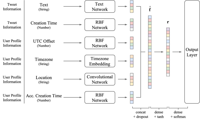
Figure 1: Overall architecture of deepgeo.

3 Geolocation Prediction

3.1 Dataset

We use the geolocation prediction shared task dataset Han et al. (2016) for our experiments. There are 2 proposed tasks, predicting geolocation given: (1) a tweet (tweet-level); and (2) a collection of tweets by a user (user-level). For each task, there is a hard classification evaluation setting for predicting a city class, and a soft evaluation setting for predicting latitude and longitude coordinates.

We explore only the more challenging tweet-level prediction task. In terms of evaluation setting, we experiment with the hard classification setting, where the network is required to predict one out of 3362 cities. Note that the metadata of a tweet includes not only the message but a variety of information such as creation time and user account data such as location and timezone.

Training, development and test partitions are provided by the shared task organisers. We preprocess the data minimally, removing tweets that have less than 5 characters in the training partition (development and testing data is untouched) and keeping all character types that have occurred 5 times or more in training. Unseen character tokens are represented by $<$UNK$>$. Preprocessed statistics of the dataset is given in Table 1.

Partition	#Tweets	#Characters
Training	8.9M	554M
Development	7.2K	439K
Test	10K	629K

Table 1: Dataset statistics.

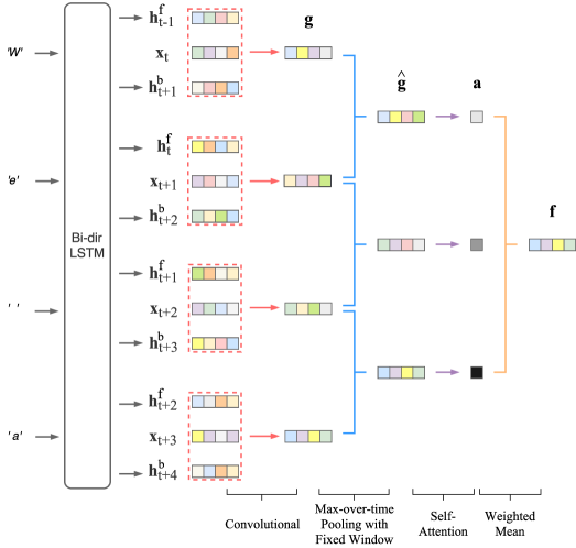
Figure 2: Text Network.

3.2 Network Architecture

The overall architecture of our model (henceforth deepgeo) is illustrated in Figure 1. deepgeo uses 6 features from the metadata: (1) tweet message; (2) tweet creation time; (3) user UTC offset; (4) user timezone; (5) user location; and (6) user account creation time.

Each feature from the metadata is processed by a separate network to generate a feature vector $\mathbf{f}_{j}$. These feature vectors are then concatenated (with dropout applied) and connected to the penultimate layer:

$$\hat{\mathbf{f}} =\mathbf{f}_{1}\oplus\mathbf{f}_{2}...\oplus\mathbf{f}_{N}$$ (1)

$$\mathbf{r} =\text{tanh}(\mathbf{W}_{r}\hat{\mathbf{f}})$$ (2)

where $N$ is the number of features (6 in total), $\mathbf{r}\in\mathbb{R}^{R}$ is the hidden representation at the penultimate layer and $\mathbf{W}_{r}$ is model parameter. For brevity, we omit biases in equations.

$\mathbf{r}$ is fully connected to the output layer and activated by softmax to generate a probability distribution over the classes. The model is trained with minibatches and optimised using Adam (Kingma and Ba, 2014) with standard cross-entropy loss.

We design several networks for the raw features. The first is a character-level recurrent convolutional network with a self-attention component for processing the tweet message (Section 3.2.1). The second is an RBF network for processing numbers (Section 3.2.2). The third is a simple convolutional network for processing user location (Section 3.2.3), and the last is an embedding matrix for user timezone. We treat the timezone as a categorical feature, and learn embeddings for each timezone (309 unique timezones in total). Note that these feature-processing networks are disjointed and there is no parameter sharing between them.

3.2.1 Text Network

For the tweet message, we use a character-level recurrent convolutional network Lai et al. (2015), followed by max-over-time pooling with a fixed window size and an attentional component to generate the feature vector, as illustrated in Figure 2.

Let $\mathbf{x}_{t}\in\mathbb{R}^{E}$ denote the character embedding of the $t$-th character, we run a bi-directional LSTM network Hochreiter and Schmidhuber (1997) to generate the forward and backward hidden states $\mathbf{h}^{f}_{t}$ and $\mathbf{h}^{b}_{t}$ respectively. We then concatenate the left and right context’s hidden states with $\mathbf{x}_{t}$ and generate:

$$\hat{\mathbf{x}}_{t} =\mathbf{h}^{f}_{t-1}\oplus\mathbf{x}_{t}\oplus\mathbf{h}^{b}_{t+1}$$

$$\mathbf{g}_{t} =\text{ReLU}(\mathbf{W}_{g}\hat{\mathbf{x}}_{t})$$

where $\hat{\mathbf{x}}_{t}\in\mathbb{R}^{3E}$, $\mathbf{W}_{g}\in\mathbb{R}^{O\times 3E}$ and $\mathbf{g}_{t}\in\mathbb{R}^{O}$. We iterate for each character to generate $\mathbf{g}_{t}$ for all time steps ($\mathbf{W}_{g}$ can be interpreted as $O$ convolutional filters each with a window of $3\times E$ striding 3 steps at a time). Next, we apply max-over-time (narrow) pooling with window size $P$ over the vectors:

$$\hat{\mathbf{g}}_{t}=\text{max}(\mathbf{g}_{t},\mathbf{g}_{t+1},...,\mathbf{g}_{t+P-1})$$

where $\hat{\mathbf{g}}_{t}\in\mathbb{R}^{O}$ and max is a function that returns the element-wise maxima given a number of vectors of the same length. If there are $T$ characters in the tweet, this yields $(T-P+1)$ $\hat{\mathbf{g}}$ vectors, one for each span.

By setting $P=T$, we could generate one vector for the whole tweet. The idea of using a smaller window is that it enables a self-attention component, thereby allowing the network to discover the saliency of a character span — for our task this means attending to location indicative words (Section 3.4). We define the attention network as follows:

$$\alpha_{t} =\mathbf{v}^{\intercal}\text{tanh}(\mathbf{W}_{v}\hat{\mathbf{g}}_{t})$$

$$\mathbf{a} =\text{softmax}(\alpha_{0},\alpha_{1},...,\alpha_{T-P})$$

where $\mathbf{W}_{v}\in\mathbb{R}^{V\times O}$, $\mathbf{v}\in\mathbb{R}^{V}$ and $\mathbf{a}\in\mathbb{R}^{T-P+1}$. Given the attention, we compute a weighted mean to generate the final feature vector:

$$\mathbf{f}_{\text{text}}=\sum^{T-P}_{t=0}\mathbf{a}_{t}\hat{\mathbf{g}}_{t}$$

where $\mathbf{a}_{t}$ denotes the $t$-th element in $\mathbf{a}$, and $\mathbf{f}_{\text{text}}\in\mathbb{R}^{O}$.

3.2.2 RBF Network

There are three time features in the metadata: tweet creation time, user account creation time and user UTC offset. The creation times are given in UTC time (i.e. not local time), e.g. Thu Jul 29 17:25:38 +0000 2010 and the offset is an integer.

For the creation times, we use only time of the day information (e.g. 17:25) and normalise it from 0 to 1. UTC offset is converted to hours and normalised to the same range.

The aim of the network is to split time into multiple bins. We can interpret each hour as one bin (24 bins in total) and tweets originated from a particular location (e.g.  Europe) favour certain hours or bins. This preference of bins should be different to tweets from a distant location (e.g. East Asia). Assuming each bin follows a Gaussian distribution, then the goal of the network is to learn the Gaussian means and standard deviations of the bins.

Formally, given an input value $u$, for bin $i$ the network computes:

$$r_{i}=\exp\left(\frac{-(u-\mu_{i})^{2}}{2\sigma_{i}^{2}}\right)$$

where $r_{i}$ is the output value and $\mu_{i}$ and $\sigma_{i}$ are the parameters for bin $i$. Let $B$ be the total number of bins, the feature vector generated by a RBF network is given as follows:

$$\mathbf{f}_{\text{rbf}}=[r_{0},r_{1},...,r_{B-1}]$$

where $\mathbf{f}_{\text{rbf}}\in\mathbb{R}^{B}$.

3.2.3 Convolutional Network

Location is a user self-declared field in the metadata. As it is free-form text, we use a standard character-level convolution neural network Kim (2014) to process it. The network architecture is simpler compared to the text network (Section 3.2.1): it has no recurrent and self-attention layers, and max-over-time pooling is performed over all spans.

Let $\mathbf{x}_{t}\in\mathbb{R}^{E}$ denote the character embedding of the $t$-th character in the tweet. A tweet of $T$ characters is represented by a concatenation of its character vectors: $\mathbf{x}_{0:T-1}=\mathbf{x}_{0}\oplus\mathbf{x}_{1}\oplus...\oplus\mathbf{x}_{T-1}$. We use convolutional filters and max-over-time (narrow) pooling to compute the feature vector:

$$\mathbf{g}_{t} =\text{ReLU}(\mathbf{W}_{g}\mathbf{x}_{t:t+Q-1})$$

$$\mathbf{f}_{\text{conv}} =\text{max}(\mathbf{g}_{0},\mathbf{g}_{1},...,\mathbf{g}_{T-Q})$$

where $Q$ is the length of the character span, $\mathbf{W}_{g}\in\mathbb{R}^{O\times QE}$ ($\mathbf{W}_{g}$ can be interpreted as $O$ convolutional filters each with a window of $Q\times E$) and $\mathbf{g}_{t},\mathbf{f}_{\text{conv}}\in\mathbb{R}^{O}$.

3.3 Experiments and Results

We explore two sets of features for predicting geolocation, using: (1) only the tweet message; and (2) both tweet and user metadata. For the latter approach, we have 6 features in total (see Figure 1). Classification accuracy is used as the metric for evaluation.

We tune network hyper-parameter values based on development accuracy; optimal hyper-parameter settings are presented in Table 2. The column “Message-Only” uses only the text content of tweets, while “Tweet$+$User” incorporates both tweet and user account metadata.

For tweet message and user location, the maximum character length is set to 300 and 20 characters respectively; strings longer than this threshold are truncated and shorter ones are padded. Models are trained using 10 epochs without early stopping. In each iteration, we reset the model’s parameters if its development accuracy is worse than that of previous iteration.

We compare deepgeo to 3 benchmark systems, all of which are systems submitted to the shared task Han et al. (2016):

Network Hyper- Message- Tweet$+$ Parameter Only User Overall Batch Size 512 Epoch No. 10 Dropout 0.2 Learning Rate 0.001 $R$ 400 Text Max Length 300 300 $E$ 200 200 $P$ 10 10 $O$ 600 400 Time $B$ – 50 UTC Offset $B$ – 50 Timezone Embedding – 50 Size Location Max Length – 20 $E$ – 300 $Q$ – 3 $O$ – 300 Account $B$ – 10 Time

Table 2: deepgeo hyper-parameters and values.

Accuracy System Features 0.146 Chi et al. (2016) Message Only 0.212 deepgeo Message Only 0.409 Miura et al. (2016) Tweet $+$ User Metadata 0.428 deepgeo Tweet $+$ User Metadata 0.436 Jayasinghe et al. (2016) Tweet $+$ User Metadata, Gazetteer, URL IP Lookup, Label Prop. Network

Table 3: Geolocation prediction test accuracy.

Tweet True Predicted 1st Span 2nd Span 3rd Span Label Label Big thanks to @LouSnowPlow and all #CleanSidewalk participants today. You really make Louisville shine. To be happy, be compassionate! louisville- ky111-us louisville- ky111-us ‘Louisville’ ‘ake Louisv’ ‘ Louisvill’ McDonald’s with aldha (@ Jalan A. P. Pettarani) http://t.co/HDVkhsKWBa makassar-38-id makassar-38-id ‘Pettarani)’ ‘ Pettarani’ ‘ettarani) ’ Let’s miss ALL the green lights on purpose! - every driver in Moncton this morning moncton-04-ca halifax-07-ca ‘in Moncton’ ‘ncton this’ ‘Moncton th’ Harrys bar toilet selfie @sophiethielmann @ Carluccio’s Newcastle https://t.co/rKT7RGe7Nd newcastle upon tyne-engi7-gb newcastle upon tyne-engi7-gb ‘s Newcastl’ ‘wcastle ht’ ‘castle htt’ Makan terossssssss  wkwkwk (with Erwina and Indah at McDonald’s Bintara) - https://t.co/lT3KERFgap bekasi-30-id bekasi-30-id ‘ Bintara) ’ ‘ntara) - h’ ‘intara) - ’ @EileenOttawa For better or worse it’s a revenue stream for Twitter made available to businesses. We all have to get used to it. toronto-08-ca ottawa-08-ca ‘tawa For b’ ‘ttawa For ’ ‘nOttawa Fo’ Hunt work!! (with @hadiseptiandani and @Febriantivivi at Jobforcareer Senayan) - https://t.co/u9myRDidtR jakarta-04-id jakarta-04-id ‘nayan) - h’ ‘ Senayan) ’ ‘enayan) - ’

Table 4: Examples of top character spans. Length of span is 10 characters. “1st Span” denotes the span that has the highest attention weight, “2nd Span” and “3rd Span” the second and third highest weight respectively.

Feature Set	Accuracy
All Features	0.428
$-$Text	0.342	($-$0.086)
$-$Tweet Creation Time	0.419	($-$0.009)
$-$UTC Offset	0.431	($+$0.003)
$-$Timezone	0.422	($-$0.006)
$-$Location	0.228	($-$0.200)
$-$Account Creation Time	0.424	($-$0.004)

Table 5: Feature ablation results.

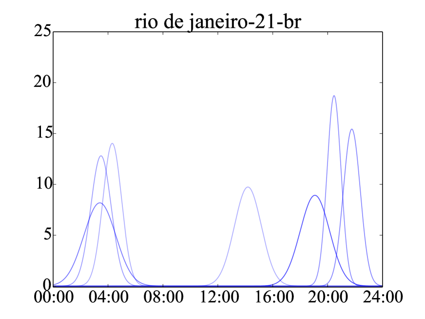
(a) UTC-03

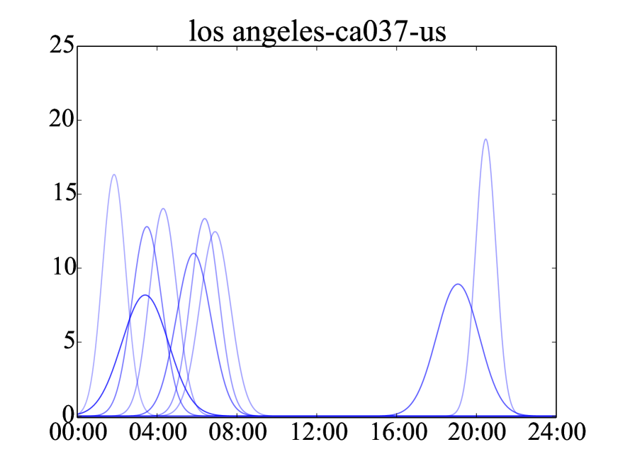
(b) UTC-07

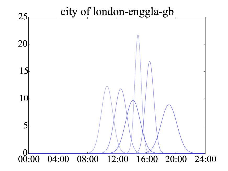
(c) UTC+00

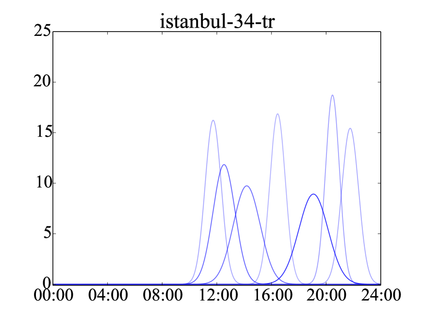
(d) UTC+03

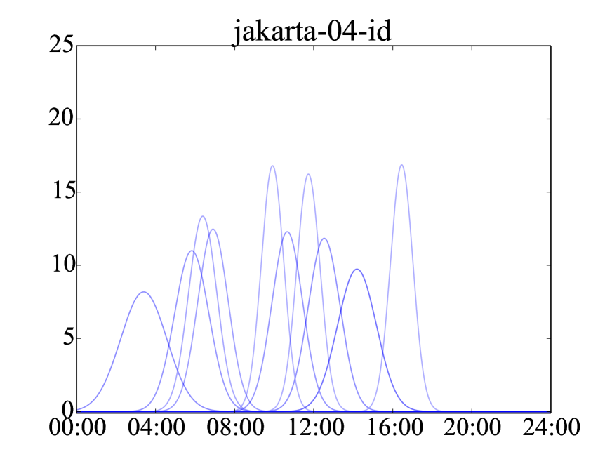
(e) UTC+07

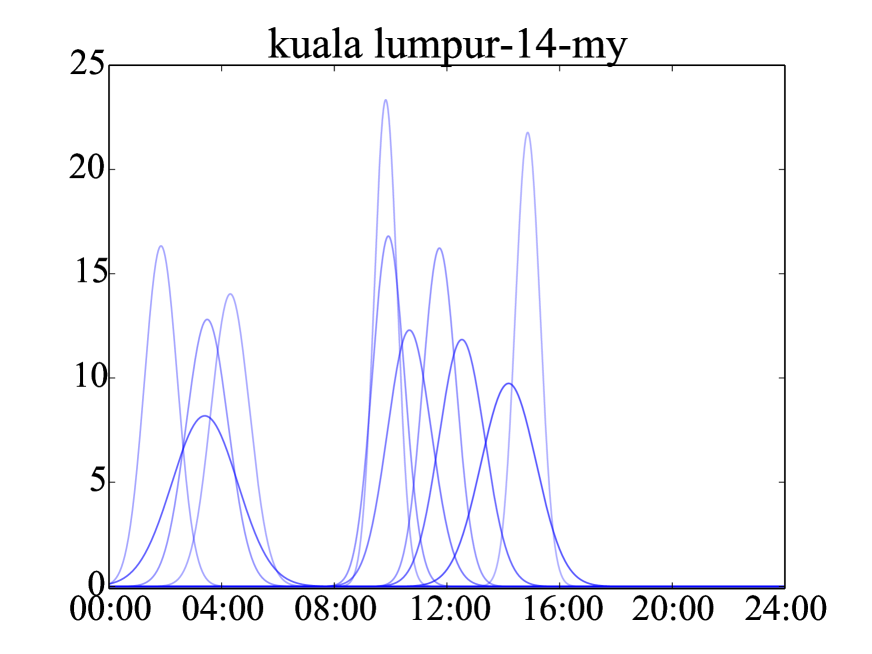
(f) UTC+08

Figure 3: Tweet creation time distribution for 6 cities. Times in all plots are in UTC time. Sub-caption indicates a city’s UTC offset.

Chi et al. (2016)

propose a geolocation prediction approach based on a multinomial naive Bayes classifier using a combination of automatically learnt location indicative words, city/country names, #hashtags and @mentions. A frequency-based feature selection strategy is used to select the optimal subset of word features.

Miura et al. (2016)

experiment with a simple feedforward neural network for geolocation classification. The network draws inspiration from fastText Joulin et al. (2016), where it uses mean word vectors to represent textual features and has only linear layers. To incorporate multiple features — tweet message, user location, user description and user timezone — the network combines them via vector concatenation.

Jayasinghe et al. (2016)

develop an ensemble of classifiers for the task. Individual classifiers are built using a number of features indepedently from the metadata. In addition to using information embedded in the metadata, the system relies on external knowledgebases such as gazetteer and IP look up system to resolve URL links in the message. They also build a label propagation network that links connected users, as users from a sub-network are likely to come from the same location. These classifiers are aggregated via voting, and weights are manually adjusted based on development performance.

We present test accuracy performance for all systems in Table 3. Using only tweet message as feature, deepgeo outperforms Chi et al. (2016) by a considerable margin (over 6% improvement), even though deepgeo has minimal feature engineering and is trained at character level. Next, we compare deepgeo to Miura et al. (2016). Both systems use a similar set of features from the tweet and user metadata. deepgeo sees an encouraging performance, with almost 2% improvement. The best system in the shared task, Jayasinghe et al. (2016), remains the top performer. Note, however, that their system depends on language-specific processing tools (e.g. tokenisers), website-specific parsers (e.g. for extracting location information from user profile page on Instagram and Facebook) and external knowledge sources (e.g. gazetteers and IP lookup) which were inaccessible by other systems.

To better understand the impact of each feature, we present ablation results where we remove one feature at a time in Table 5. We see that the two most important features are the user location and tweet message. These observations reveal that self-declared user location appears to be a reliable source of location, as task accuracy drops by almost half when this feature is excluded. For the other features, they generally have a small or negligible impact.

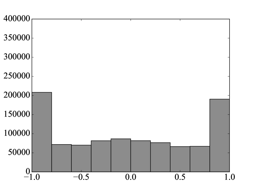
(a) 100; 0.0; 0.0

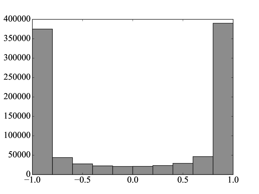
(b) 100; 0.1; 0.0

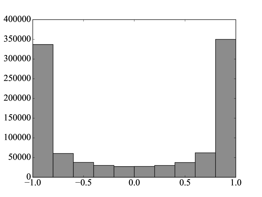
(c) 100; 0.0; 0.1

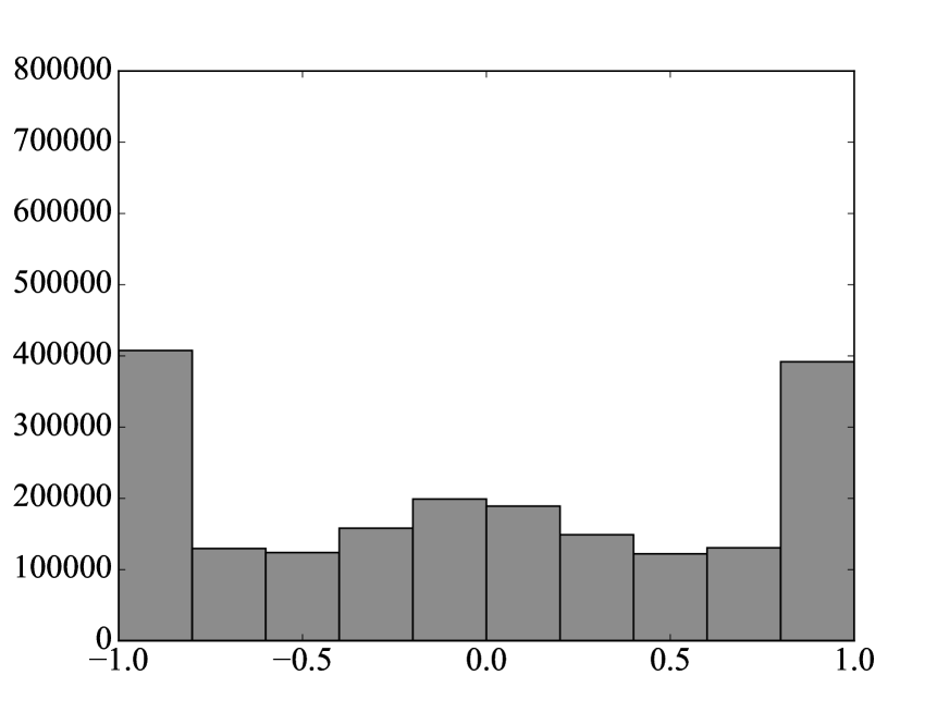
(d) 200; 0.0; 0.0

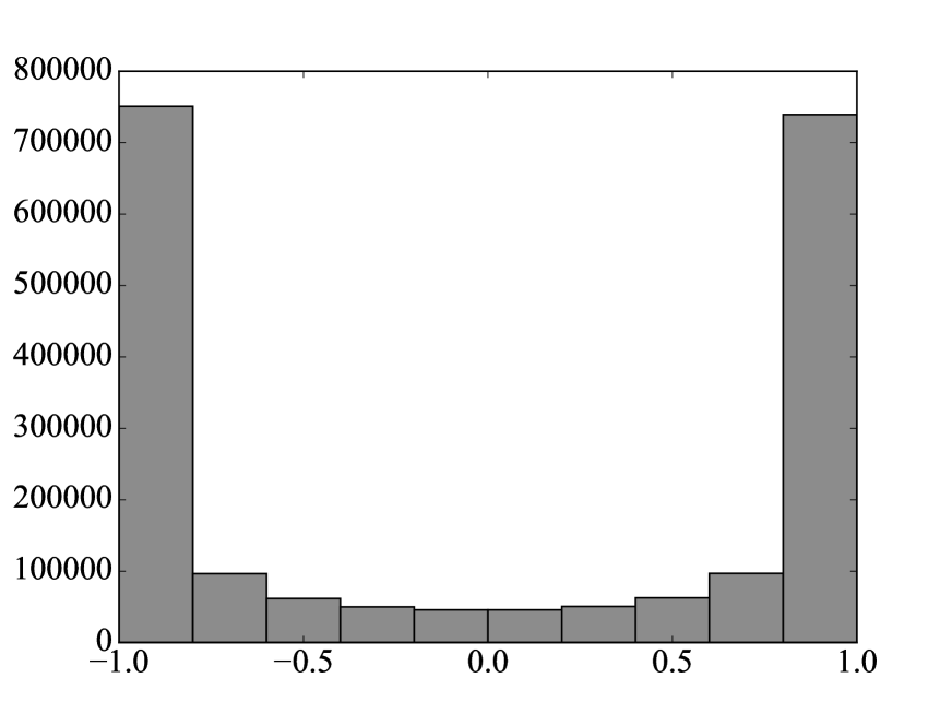
(e) 200; 0.1; 0.0

(f) 200; 0.0; 0.1

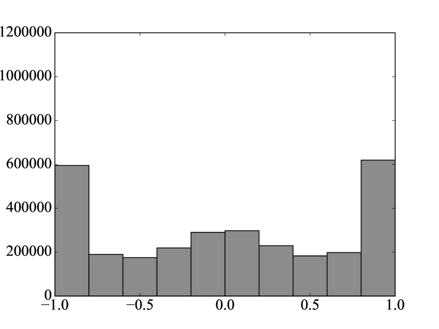
(g) 300; 0.0; 0.0

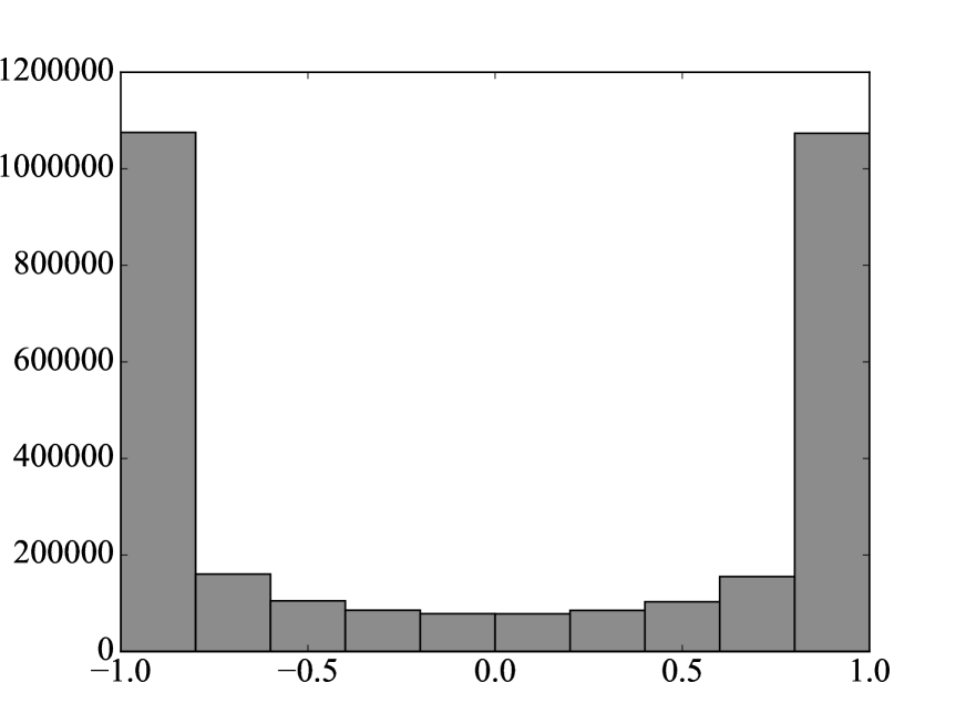
(h) 300; 0.1; 0.0

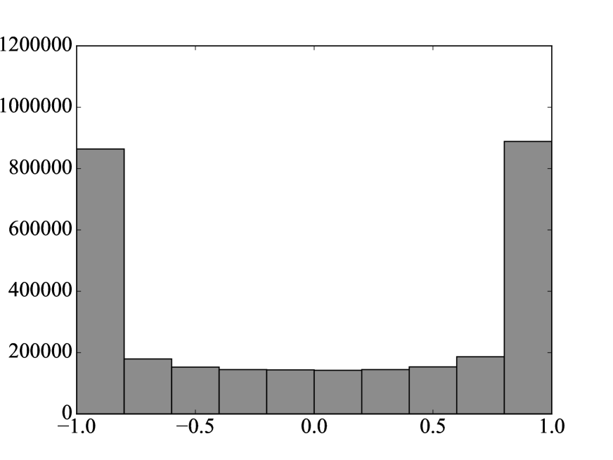
(i) 300; 0.0; 0.1

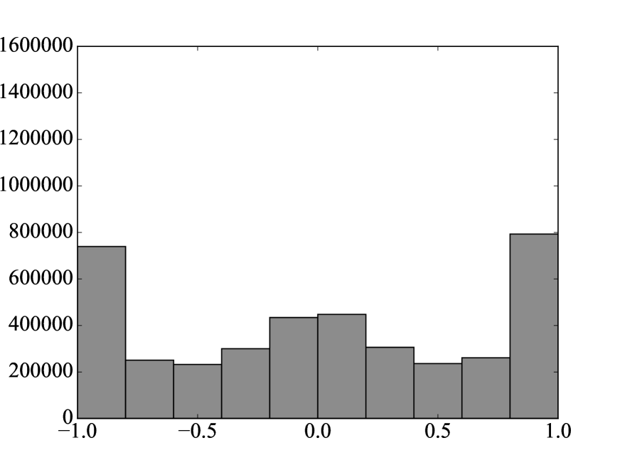
(j) 400; 0.0; 0.0

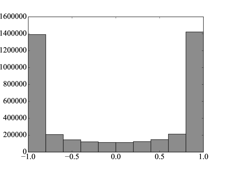
(k) 400; 0.1; 0.0

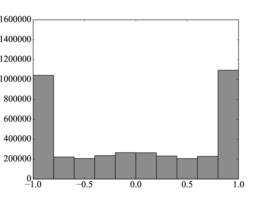
(l) 400; 0.0; 0.1

Figure 4: Histogram of $\mathbf{r}$ element values. Fields in the subcaptions denote vector dimension ($R$), corruption level ($\sigma$) and $l$ scaling factor ($\alpha$). Range of y-axis for the same vector dimension is standardised.

3.4 Qualitative Analyses

The self-attention component in the text network (Section 3.2.1) captures saliency of character spans. To demonstrate its effectiveness, we select a number of tweets from the test partition and present the top-3 spans that have the highest attention weights in Table 4.

Interestingly, we see that whenever a location word is in the message, deepgeo tends to focus around it (e.g. Louisville and Newcastle). Occasionally this can induce error in prediction, e.g. in the second last example the network focuses on Ottawa even though the word has little significance to the true location (Toronto). Focussing on the right span does not necessarily result in correct prediction as well; as we see in the third example the network focuses on Moncton but predicts a neighbouring city Halifax as the geolocation.

Next, we look at the Gaussian mixtures learnt by the RBF network. Using the gold-standard city labels, we collect bin weights ($\mathbf{f}_{\text{rbf}}$) for tweet creation times (from test data) for 6 cities and plot them in Figure 3. Each Gaussian distribution represents one bin, and its weight is computed as a mean weight over all tweets belonging to the city (line transparency indicates bin weight). Bins that have a mean weight $<0.075$ are excluded.

For London (Figure 3(c)), we see that most tweets are created from 10:00–20:00 local time. For Jakarta (Figure 3(e)), tweet activity mostly centers around 11:00–23:00 local time (04:00–16:00 UTC time). Most cities share a similar activity period, with the exception of Istanbul (Figure 3(d)): Turkish people seems to start their day much later, as tweets begin to appear from 15:00–01:00 local time (12:00 to 22:00 UTC time).

Another interesting trend we find is that for two cities (Los Angeles and Kuala Lumpur), there is a brief period of inactivity around noon (12:00) to evening (18:00) in local time. We hypothesise that most people are working during these times, and are thus too busy to use Twitter.

4 Hashing: Generating Binary Code For Tweets

Bits deepgeo deepgeo deepgeo lsh fasthash $+$noise $+$loss word2vec deepgeo word2vec deepgeo 100 0.147 0.149 0.146 0.013 0.053 0.116 0.140 200 0.143 0.143 0.140 0.019 0.072 0.128 0.160 300 0.136 0.137 0.141 0.021 0.082 0.133 0.165 400 0.132 0.135 0.136 0.022 0.086 0.135 0.170

Table 6: Retrieval MAP performance.

deepgeo creates a low-dimensional dense vector representation ($\mathbf{r}$) for a tweet in the penultimate layer. This representation captures the message, user timezone and other metadata (including the city label) that are incorporated to the network during training.

Storing the dense vector representation for a large volume of tweets can be costly. If we can compress the dense vectors into compact binary codes, it would save storage space, as well as enabling more efficient retrieval of co-located tweets, e.g. using multi-index hash tables for $K$-nearest neighbour search Norouzi et al. (2012, 2014).

Inspired by denoising autoencoders Yu et al. (2016); Vincent et al. (2010), we binarise the dense vector generated by deepgeo by adding Gaussian noise. The intuition is that the addition of noise sharpens the activation values in order to counteract the random noise.

Equation (1) is thus modified to: $\hat{\mathbf{f}}=(\mathbf{f}_{1}\oplus\mathbf{f}_{2}...\oplus\mathbf{f}_{N})+\mathcal{N}(0,\sigma^{2})$, where $\mathcal{N}(0,\sigma^{2})$ is a zero-mean Gaussian noise with standard deviation (or corruption level) $\sigma$.

$R$ deepgeo deepgeo deepgeo $+$noise $+$loss 100 0.420 0.396 0.410 200 0.428 0.417 0.414 300 0.420 0.416 0.422 400 0.428 0.419 0.418

Table 7: Classification performance for deepgeo with the addition of noise and loss term $l$.

In the addition to the Gaussian noise, we also experiment with an additional loss term $l$ to penalise elements that are not in the extrema: $l=\alpha\times\frac{1}{R}\sum_{i=0}^{R-1}|(\mathbf{r}_{i}-1)(\mathbf{r}_{i}+1)|$, where $\mathbf{r}_{i}$ is the $i$-th element in $\mathbf{r}$ and $\alpha$ is a scaling factor. We set $\sigma=\alpha=0.1$, as both values were found to provide good performance.

To better understand the effectiveness of the noise and loss term $l$ in binarising the vector values, we present a histogram plot of $\mathbf{r}$ element values from test data in Figure 4, for $R=100,200,300,400$. We see that the addition of noise and $l$ helps in pushing the elements to the extrema. The noise term appears to work a little better than $l$, as the frequency for the $-1.0$ and $+1.0$ bins is higher. We also observe that there is a small increase in middle/zero values as R increases from 100 to 400, suggesting that there are more unused hidden units when number of parameters increases. We present classification accuracy performance when we add noise (deepgeo$+$noise) and $l$ (deepgeo$+$loss) in Table 7. The performance drops a little, but generally stays within a gap of 1%. This suggests that both noise and $l$ works well in binarising $\mathbf{r}$ without trading off classification accuracy significantly.

Next we evaluate the retrieval performance using the binary codes. We binarise $\mathbf{r}$ for development and test tweets using the sign function. Given a test tweet, we retrieve the nearest development tweets based on hamming distance, and calculate average precision. We aggregate the retrieval performance for all test tweets by computing mean average precision (MAP).

For comparison, we experiment with two hashing techniques: lsh Indyk and Motwani (1998) and fasthash Lin et al. (2014) (see Section 2 for system descriptions). The input required for both lsh and fasthash is a vector. We test 2 types of input for these methods: (1) a word2vec baseline, where we concatenate mean word vectors of the tweet message, user account’s timezone and location, resulting in a $900$-dimension vector; and (2) deepgeo representation $\mathbf{r}$. The rationale for using deepgeo as input is to test whether its representation can be further compressed with these hashing techniques.

We present MAP performance for all systems in Table 6. Looking at deepgeo systems (column 2–4), we see that adding noise and $l$ helps, although the impact is greater when the bit size is large (300/400 bits). For lsh, which uses no label information, word2vec input produces poor binary code for retrieval. Changing the input to deepgeo improves retrieval considerably, implying that the representation produced by deepgeo captures geolocation information.

fasthash with word2vec input vector performs competitively. For smaller bit sizes (100 or 200), however, the gap in performance is substantial. Pairing fasthash with deepgeo produces the best retrieval performance: for 200/300/400 bits it outperforms deepgeo$+$noise by 2–4%. Interestingly for 100 bits fasthash is unable to compress deepgeo’s representation any further, highlighting the compactness of deepgeo representation for smaller bit sizes.

5 Conclusion

We propose an end-to-end method for tweet-level geolocation prediction. We found strong performance, outperforming comparable systems by 2-6% depending on the feature setting. Our model is generic and has minimal feature engineering, and as such is highly portable to problems in other domains/languages (e.g. Weibo, a Chinese social platform, is one we intend to explore). We propose simple extensions to the model to compress the representation learnt by the network into binary codes. Experiments demonstrate its compression power compared to state-of-the-art hashing techniques.

References

- Backstrom et al. (2010) L. Backstrom, E. Sun, and C. Marlow. 2010. Find me if you can: improving geographical prediction with social and spatial proximity. In Proceedings of the 19th international conference on World wide web, pages 61–70. ACM.
- Chang et al. (2012) H. Chang, D. Lee, M. Eltaher, and J. Lee. 2012. @ phillies tweeting from philly? predicting twitter user locations with spatial word usage. In Proceedings of the 2012 International Conference on Advances in Social Networks Analysis and Mining (ASONAM 2012), pages 111–118. IEEE Computer Society.
- Cheng et al. (2010) Z. Cheng, J. Caverlee, and K. Lee. 2010. You are where you tweet: a content-based approach to geo-locating twitter users. In Proceedings of the 19th ACM international conference on Information and knowledge management, pages 759–768. ACM.
- Chi et al. (2016) L. Chi, K.H. Lim, N. Alam, and C. Butler. 2016. Geolocation prediction in twitter using location indicative words and textual features. In Proceedings of the 2nd Workshop on Noisy User-generated Text (WNUT), pages 227–234, Osaka, Japan.
- Chi and Zhu (2017) L. Chi and X. Zhu. 2017. Hashing techniques: A survey and taxonomy. ACM Computing Surveys (CSUR), 50(1):11.
- Han et al. (2016) B. Han, A. Rahimi, L. Derczynski, and T. Baldwin. 2016. Twitter geolocation prediction shared task of the 2016 workshop on noisy user-generated text. In Proceedings of the 2nd Workshop on Noisy User-generated Text (WNUT), pages 213–217, Osaka, Japan.
- Han et al. (2012) Bo Han, Paul Cook, and Timothy Baldwin. 2012. Geolocation prediction in social media data by finding location indicative words. pages 1045–1062, Mumbai, India.
- Han et al. (2014) Bo Han, Paul Cook, and Timothy Baldwin. 2014. Text-based Twitter user geolocation prediction. 49:451–500.
- Hochreiter and Schmidhuber (1997) S. Hochreiter and J. Schmidhuber. 1997. Long short-term memory. Neural Computation, 9:1735–1780.
- Indyk and Motwani (1998) P. Indyk and R. Motwani. 1998. Approximate nearest neighbors: towards removing the curse of dimensionality. In Proceedings of the thirtieth annual ACM symposium on Theory of computing, pages 604–613. ACM.
- Jayasinghe et al. (2016) G. Jayasinghe, B. Jin, J. Mchugh, B. Robinson, and S. Wan. 2016. Csiro data61 at the wnut geo shared task. In Proceedings of the 2nd Workshop on Noisy User-generated Text (WNUT), pages 218–226, Osaka, Japan.
- Joulin et al. (2016) A. Joulin, E. Grave, P. Bojanowski, and Mikolov T. 2016. Bag of tricks for efficient text classification. CoRR, abs/1607.01759.
- Jurgens et al. (2015) D. Jurgens, T. Finethy, J. McCorriston, Y.T. Xu, and D. Ruths. 2015. Geolocation prediction in twitter using social networks: A critical analysis and review of current practice. In Proceedings of the Ninth International Conference on Web and Social Media, ICWSM 2015, pages 188–197, Oxford, UK.
- Kim (2014) Y. Kim. 2014. Convolutional neural networks for sentence classification. pages 1746–1751, Doha, Qatar.
- Kingma and Ba (2014) Diederik P. Kingma and Jimmy Ba. 2014. Adam: A method for stochastic optimization. CoRR, abs/1412.6980.
- Laere et al. (2014) Olivier Van Laere, Jonathan Quinn, Steven Schockaert, and Bart Dhoedt. 2014. Spatially-aware term selection for geotagging. IEEE Transactions on Knowledge and Data Engineering, 26(1):221–234.
- Lai et al. (2015) S. Lai, L. Xu, K. Liu, and J. Zhao. 2015. Recurrent convolutional neural networks for text classification. pages 2267–2273, Austin, Texas.
- Lin et al. (2014) G. Lin, C. Shen, Q. Shi, A. van den Hengel, and D. Suter. 2014. Fast supervised hashing with decision trees for high-dimensional data. In Proceedings of the IEEE Conference on Computer Vision and Pattern Recognition, pages 1963–1970.
- Miura et al. (2016) Y. Miura, M. Taniguchi, T. Taniguchi, and T. Ohkuma. 2016. A simple scalable neural networks based model for geolocation prediction in twitter. In Proceedings of the 2nd Workshop on Noisy User-generated Text (WNUT), pages 235–239, Osaka, Japan.
- Norouzi et al. (2012) M. Norouzi, A. Punjani, and D.J. Fleet. 2012. Fast search in hamming space with multi-index hashing. In Computer Vision and Pattern Recognition (CVPR), 2012 IEEE Conference on, pages 3108–3115. IEEE.
- Norouzi et al. (2014) M. Norouzi, A. Punjani, and D.J. Fleet. 2014. Fast exact search in hamming space with multi-index hashing. IEEE transactions on pattern analysis and machine intelligence, 36(6):1107–1119.
- Rahimi et al. (2015) Afshin Rahimi, Duy Vu, Trevor Cohn, and Timothy Baldwin. 2015. Exploiting text and network context for geolocation of social media users. pages 1362–1367, Denver, USA.
- Sloan et al. (2013) L. Sloan, J. Morgan, W. Housley, M. Williams, A. Edwards, P. Burnap, and O. Rana. 2013. Knowing the tweeters: Deriving sociologically relevant demographics from twitter. Sociological research online, 18(3):7.
- Vincent et al. (2010) P. Vincent, H. Larochelle, I. Lajoie, Y. Bengio, and P. Manzagol. 2010. Stacked denoising autoencoders: Learning useful representations in a deep network with a local denoising criterion. Journal of Machine Learning Research, 11:3371–3408.
- Yu et al. (2016) Z. Yu, H. Wang, X. Lin, and M. Wang. 2016. Understanding short texts through semantic enrichment and hashing. In 2016 IEEE 32nd International Conference on Data Engineering (ICDE), pages 1552–1553, Helsinki, Finland.