A Goodness-of-Fit Test for Sampled Subgraphs

Abstract

We consider the problem of testing whether a graph’s degree distribution belongs to a particular family, such as poisson or scale-free, given that we only observe a sampled subgraph. In particular, we focus on induced subgraph sampling, a sampling design which systematically distorts the degree distribution of interest. We estimate the parameter indexing the hypothesized family by generalized method of moments and utilize the Kolmogorov-Smirnov test statistic to assess goodness-of-fit. Since the distribution in the null hypothesis has been estimated, critical values for the test statistic must be simulated. We propose a novel bootstrap in which we construct a graph whose degree distribution conforms to the null hypothesis from which we may draw pseudo-samples in the form of induced subgraphs. We investigate the properties of this procedure with a monte carlo study which confirms that the bootstrap is able to attain size close to the nominal level while exhibiting power under the alternative hypothesis. We present an application of this test to the protein interaction network (PIN) of the yeast Saccharomyces cerevisiae. Accounting for the high rates of false negatives present in PIN measurement, we are able to reject the hypothesis that the PIN of S. cerevisiae follows an Erdős-Rényi random graph family of degree distributions.

T1I’d like to thank Firmin Doko Tchatoka, Simon Fielke, Petra Kuhnert, and Virginie Masson for their helpful comments.

,

1 Introduction

The degree distribution is one of the fundamental descriptions of a graph, often leading to models of network formation being referred to by their resulting degree distributions (Newman et al.,, 2001). Scale-free graphs, whose degree distributions obey a power law, are especially interesting as they exhibit a “robust-yet-fragile” property in which the graph is resilient to the failure of randomly selected vertices but vulnerable to catastrophic failure in the event that its high-degree hubs are targeted (Albert et al.,, 2000; Doyle et al.,, 2005). This feature is common to many real-world graphs, such as interbank lending networks and the webgraph of the internet (Boss et al.,, 2004; Gai et al.,, 2011; Doyle et al.,, 2005).

We consider the problem of testing the hypothesis that a graph’s degree distribution belongs to a particular family, such as poisson or power law, based on a sampled subgraph but without requiring that the hypothesized distribution be fully parameterized. This is akin to Lilliefors, (1967, 1969). Supposing that an i.i.d sample of degrees were acquired, this would be a standard goodness-of-fit test with critical values computable with the bootstrap.However, graphs are often sampled in a fashion where observed degrees may not be considered i.i.d draws from the population (Kolaczyk,, 2009, Chapter 5).

Here we consider samples acquired to be induced subgraphs. Induced subgraph sampling involves randomly sampling a subset of vertices without replacement and retaining only the edges in the population between the vertices sampled. This sampling design systematically distorts the degree distribution as vertices with high degree are more likely to have neighbors included in the sample, and therefore an edge included, than vertices with low degree. Figure 1 illustrates this procedure. Nonparametric estimation of the degree distribution based on induced subgraph samples, which has been considered by Frank, (1980) and Zhang et al., (2015), has proven to be particularly challenging.

(a) Population Graph

(b) Induced Subgraph

Figure 1: 1(a) shows a graph representing a population of ten vertices where six vertices have been selected through simple random sampling. 1(b) displays the subgraph induced by those vertices.

In this article we propose a novel bootstrap which allows for critical values to be simulated for a goodness-of-fit test when the sample acquired is an induced subgraph. We propose estimating the parameter indexing the hypothesized family of distributions using generalized method of moments (GMM), for which we exploit a moment condition from Frank, (1980) and an approximation to its covariance matrix from Zhang et al., (2015). Once the null distribution has been estimated, we construct a graph whose degree distribution conforms to the null hypothesis from which we may draw pseudo-samples in the form of induced subgraphs. We conduct a monte carlo experiment for poisson and power law data generating processes to assess the size and power properties of the test for various sampling rates. We confirm that the bootstrap is able to control the size of the test close to the nominal level while exhibiting power under most alternatives. However, in some regions of the parameter space the test is unable to distinguish between the two DGPs, particularly for small sampling rates.

We apply this test to the protein interaction network (PIN) of the budding yeast Saccharomyces cerevisiae. One of the common methods for measuring PINs, the yeast two-hybrid assay (Y2H), detects pairwise interactions between a set of sampled proteins. Thus, PINs that result from Y2H assays constitute induced subgraph samples. The degree distribution of a PIN is an especially interest feature of the network as the degree of a protein in the network has been noted to correlate with its essentiality for the viability of a cell or organism (Jeong et al.,, 2001). If the degree distribution of a PIN followed a power law, with many sparsely connected vertices and only a few highly connected, then therapies which target the function of a highly connected protein present a strategy for medical interventions (Vogelstein et al.,, 2000). If the PIN’s degree distribution is more like than of an Erdős-Rényi random graph, then such a strategy wouldn’t be expected to be as successful.

Y2H assays are prone to significant measurement error, plagued by high rates of both false positives and negatives. Han et al., (2005) show via simulation study that when such measurement error is introduced, subgraphs formed by scale-free and poisson graphs can be practically indistinguishable. In our application we consider five data sets from Yu et al., (2008), for which each is believed to have high specificity but low sensitivity. We explicitly incorporate various frequencies of type I error into our test and are able to reject the hypothesis that the S. cerevisiae PIN follows a poisson distribution for each.

2 Setup

Let $G=(V,E)$ be a simple graph with $|V|=N$ vertices. $\{i,j\}\in E$ if there is an undirected edge between vertices $i$ and $j$. The degree of vertex $i$, $d_{i}(G)=\sum_{j\not=i}I(\{i,j\}\in E)$, is the number of vertices with which $i$ shares an edge. The degree distribution of $G$ is a vector, $P_{G}\in\mathbb{R}^{N}$, containing the frequency with which vertices of a particular degree occur, $P_{G}(k)=\#\{i:d_{i}=k\}/N$, $k=0,\dots,N-1$. The cumulative distribution function (CDF) may be defined as usual $F_{G}(k)=\sum_{i\leq k}P_{G}(i)$. Let $G^{\prime}=(V^{\prime},E^{\prime})$ be an induced subgraph formed by random sampling $|V^{\prime}|=n$ vertices and including an edge $\{i,j\}\in E^{\prime}$ if and only if $i,j\in V^{\prime}$.

Let $F_{0}(\theta)$ be a family of distributions indexed by an unknown parameter vector $\theta$. The objective is to test the following hypothesis.

$$H_{0}:F_{G}=F_{0}(\theta)\quad vs.\quad H_{A}:F_{G}\not=F_{0}(\theta)$$ (1)

That is, we are looking to perform a goodness-of-fit test against a family of distributions. For example, we may wish to detect whether the population graph $G$ follows one of the common network distributions, such as poisson or a power law. Standard goodness-of-fit tests for which critical values may be tabulated for the test statistics, such as Kolmogorov-Smirnov or Pearson’s Chi-square, require that the hypothesised distribution be fully specified. However, we do not have a priori knowledge of the parameter vector $\theta$ and must estimate it from the sampled subgraph $G^{\prime}$. This is akin to Lilliefors, (1967, 1969) in that critical values must be extracted through monte carlo simulation.

An added difficulty lies in the sampling method. Supposing that a random sample of the degrees of vertices in $G$ were acquired, simulation of the critical values would be relatively straightforward. However, the sample consists of an induced subgraph, wherein the degree of vertices is systematically distorted by measuring edges only to other vertices in the sample. This presents an issue both in the simulation of critical values and in the estimation of the parameter $\theta$.

2.1 Estimation

Supposing we draw an induced subgraph sample of size $n$ from a population graph on $N$ vertices, it is relatively easy to show that the distortion to the degree distribution obeys the following.

$$\mathbb{E}[P_{G^{\prime}}]=\bm{X}P_{G}$$ (2)

where

$$\bm{X}_{ij}=\binom{j}{i}\binom{N-1-j}{n-1-i}\binom{N-1}{n-1}^{-1}$$ (3)

for $i,j$ such that the binomial coefficients are defined and $\bm{X}_{ij}=0$ otherwise. This is assuming that a subset of $n$ vertices is selected by simple random sampling. In the case of Bernoulli sampling, where each vertex is selected to be in the sample independently with probability $p$, then the columns of the design matrix would be binomial distributions rather than hypergeometric.

It’s important to note that $\bm{X}$ has dimensions $n\times N$, with $N\gg n$, so direct estimation of $P_{G}$ via least squares is infeasible. Frank, (1980) constructs an unbiased estimator for $P_{G}$ by assuming a known maxmum degree in the population graph, allowing for the matrix $\bm{X}$ to be truncated such that it becomes square. However, this estimator exhibits extreme estimates, far outside the admissible $[0,1]$ interval, and erratic sign switching behavior. Zhang et al., (2015) identify the origin of this pathological behavior as the design matrix being severely ill-conditioned with singular values decaying quickly to zero. They propose stabilizing the inversion of $\bm{X}$ by using Tikhonov regularization and imposing that the estimate be a valid probability mass by constraint. They choose the tuning parameter in the penalty term using a monte carlo version of Stein’s unbiased risk estimate (Stein,, 1981; Ramani et al.,, 2008; Eldar,, 2009). Here we are able to avoid issues with estimating $P_{G}$ directly as long as the vector $\theta$ parameterizing the family of distributions being tested is of dimension much lower than $n$.

Zhang et al., (2015) also show that for moderate sampling rates, the sampling error term in the linear system

$$P_{G^{\prime}}=\bm{X}P_{G}+\bm{\varepsilon}$$ (4)

may be well approximated by $\bm{\varepsilon}\sim N\left(0,\frac{1}{n}\text{diag}(\bm{X}P_{G})\right)$.

Let $P_{0}(\theta)$ be the probability mass corresponding to the hypothesized distribution $F_{0}(\theta)$. In order to estimate $\theta$ from the induced subgraph sample $G^{\prime}$, we exploit the moment condition in equation 2 to construct a GMM estimator.

$$\hat{\theta}=\underset{\theta}{\text{argmin}}\ n(P_{G^{\prime}}-\bm{X}P_{0}(\theta))^{\prime}\mathbf{W}(P_{G^{\prime}}-\bm{X}P_{0}(\theta))$$ (5)

where $\mathbf{W}$ denotes a weighting matrix. To perform efficient GMM the weighting matrix in 5 should be chosen to be the inverse covariance matrix of the moment condition. Using the approximation from Zhang et al., (2015) ideally we would choose

$$\mathbf{W}=\left[\text{diag}(\bm{X}P_{0}(\theta))\right]^{+}$$ (6)

where $\mathbf{A}^{+}$ denotes a pseudo-inverse of $\mathbf{A}$. It must be pseudo-inverted since many elements along the diagonal of $diag(\mathbf{X}P_{0}(\theta))$ will be zero. However, this presents an issue when estimating the parameter of scale-free and other heavy tailed distributions. Goldstein et al., (2004) show that estimating a power law parameter by linear fit on a log-log scale leads to inaccurate estimates, with maximum likelihood demonstrating superior properties. We encounter a similar difficulty in that, for power law distributions, the elements of $\mathbf{X}P_{0}(\theta)$ may not decay quickly enough to zero. This causes elements in the weighting matrix to become greatly inflated. Instead we estimate the weighting matrix using equation 2.

$$\hat{\mathbf{W}}=\left[\text{diag}(P_{G^{\prime}})\right]^{+}$$ (7)

This also guarantees that the program is convex and can be readily solved by numerical algorithms.

We can now construct our preferred test statistic for assessing goodness of fit. Common choices are the Kolmogorov-Smirnov (KS) statistic (Massey Jr,, 1951) or a statistic of squared contrasts whose null distribution is chi-square (Pearson,, 1900; Wald,, 1943). Letting $\tilde{F}_{0}(\hat{\theta})$ be the CDF of $\mathbb{E}[P_{G^{\prime}}|\ \hat{\theta}]=\bm{X}P_{0}(\hat{\theta})$, the KS statistic has the form

$$D(G^{\prime})=\sqrt{n}\sup|F_{G^{\prime}}-\tilde{F}_{0}(\hat{\theta})|$$ (8)

The Wald statistic may be found by substituting $\hat{\theta}$ into the objective function in equation 5. In what follows we focus on the KS statistic.

3 Bootstrap

Here we propose a bootstrap (Efron,, 1979) for simulating the critical values corresponding to the previously constructed statistic $D(G^{\prime})$. A typical parametric bootstrap for a Lilliefors-type test presented here would involve estimating the parameter of the hypothesized distribution, $\hat{\theta}$, drawing many pseudo-samples from the distribtution indexed by that estimate, $F_{0}(\hat{\theta})$, and constructing a bootstrap statistic $D^{*}$ for each pseudo-sample. The distribution of these bootstrap statistics may then be used to calculate P-values or critical values. The departure from standard practice here is that our sample is not an iid draw from $F_{0}$ under the null, rather it is an induced subgraph formed by randomly sampling the vertices of a graph whose degree distribution conforms to $F_{0}$. If we wish for the bootstrap to appropriately immitate the sampling process under the null, we will require a graph with degree distribution $F_{0}(\hat{\theta})$ for arbitrary $\hat{\theta}$. In order to construct a graph conforming to the null hypothesis we employ an algorithm for constructing a graph with a prescribed degree distribution due to the Configuration Model of network formation (Bender and Canfield,, 1978; Bollobás,, 1982).

Given a graph, $G_{0}$ on $N$ vertices whose degree distribution conforms to the null hypothesis, $F_{0}(\hat{\theta})$, we suggest the following bootstrap for the Kolmogorov-Smirnov statistic in equation 8.

Algorithm 1 Graphical Bootstrap

1:for $i=1\text{ to }B$ do

2:     Let $H$ be a subgraph induced on a random sample of $n$ vertices of $G_{0}$.

3:     Let $P_{H}$ be the degree distribution of $H$.

4:     $\hat{\theta}^{*}\leftarrow\underset{\theta}{\text{argmin}}\ n(P_{H}-\bm{X}P_{0}(\theta))^{\prime}\left(\text{diag}(\bm{X}P_{0}(\theta)\right)(P_{H}-\bm{X}P_{0}(\theta))$

5:     $D^{*}_{i}\leftarrow\sqrt{n}\sup|F_{H}-\tilde{F}_{0}(\hat{\theta}^{*})|$

6:end for

7:Let $c_{1-\alpha}$ be the $1-\alpha$ quantile of $\mathbb{P}_{*}(\tau\leq D^{*}_{i})$.

8:Reject $H_{0}$ if $D(G^{\prime})>c_{1-\alpha}$.

3.1 Sampling Graphs with a Prescribed Degree Distribution

Let $d_{1},\dots,d_{N}$ be the set of degrees of each vertex implied by the desired degree distribution. Begin with a set of vertices, $i=1,\dots,N$. Endow each vertex $i$, with a set of $d_{i}$ stubs (or half-edges) emanating from the vertex. Now construct a random matching on the set of stubs, and connect each pair of stubs that are matched to form an edge.

To randomly match the stubs, create a list of the vertex labels in which label $i$ appears $d_{i}$ times, then form a random permutation of the list. To construct the graph, start at the first entry in the permuted list and begin pairing off the stubs of vertices with adjacent labels.

Example 1.

Suppose we wish to construct a graph with degree sequence $4,2,2,1,1$.

Figure 2: Vertices with 4, 2, 2, 1, and 1 stubs respectively.

Construct the list: $1111223345$. Produce a random permutation:

. Connect adjacent vertices.

Figure 3: Connect the stubs.

Figure 4: Resulting Graph

Given a degree sequence, $d_{1},\dots,d_{N}$, We construct the adjacency matrix of the null graph on $N$ vertices as follows.

Algorithm 2 Null Graph

1:Let $S$ be a vector of labels $1,\dots,N$ where label $i$ has multiplicity $d_{i}$

2:$A\leftarrow zeros(N,N)$

3:$P\leftarrow randperm(S)$

4:for $i=1\text{ to }N-1$ Step 2 do

5:     $A(P(i),P(i+1))\leftarrow 1$

6:     $A(P(i+1),P(i))\leftarrow 1$

7:end for

This yields an adjacency matrix $A$ from which we may sample induced subgraphs. The adjacency matrix for the subgraph induced by the set of vertices $J\subset\{j\ |\ j=1,\dots,N\}$ may be formed from extracting the set of $J$ rows and corresponding columns from $A$.

Under this sampling method it is possible for the graph to have self-loops and multiple edges between vertices. This may either be ignored, as the probability of such an occurance is declining with the number of vertices, or the algorithm may be repeated until a simple graph is formed.

4 Simulation Study

We conduct a monte carlo study in order to assess the size and power properties of the Lilliefors-type test using the Kolmogorov-Smirnov test statistic. We consider testing for two common graph distributions: poisson random graph, and scale-free. The poisson random graph has a poisson degree distribution

$$P_{\lambda}(k)=\frac{e^{-\lambda}\lambda^{k}}{k!}$$ (9)

and may be considered the limiting degree distribution of a graph which forms through an Erdős-Rényi random graph process (Erdos and Rényi,, 1960) in which edges between vertices form independently with constant probability. A scale-free graph exhibits a power law distribution

$$P_{\gamma}(k)=\frac{k^{-\gamma}}{\zeta(\gamma)}$$ (10)

where $\zeta(\cdot)$ is the Riemann zeta function, and may be considered as forming through a preferential attachment process (Barabási and Albert,, 1999; Albert and Barabási,, 2002).

Table 1: Rejection Rates. N = 10,000.

Sampling Rate	Test Family	Data Generating Process
			Poisson
		$\lambda=1$	$\lambda=2$	$\lambda=3$	$\lambda=4$	$\lambda=5$
5%	Poisson	4.5	5.2	6.7	5.8	4.2
	Scale-free	3.7	14.1	30.0	41.4	46.0
10%	Poisson	7.9	5.4	6.4	4.1	5.0
	Scale-free	11.8	38.4	96.7	99.9	100.0
15%	Poisson	5.5	4.9	3.9	7.2	4.4
	Scale-free	28.4	77.4	100.0	100.0	100.0
20%	Poisson	4.6	5.6	6.2	4.3	6.4
	Scale-free	76.8	91.3	100.0	100.0	100.0
			Scale-free
		$\gamma=1.75$	$\gamma=2$	$\gamma=2.25$	$\gamma=2.5$	$\gamma=2.75$
5%	Poisson	14.7	12.1	9.0	6.5	3.4
	Scale-free	6.9	6.1	5.0	5.0	2.8
10%	Poisson	81.9	50.2	15.8	8.5	13.7
	Scale-free	5.6	5.0	5.6	4.9	4.2
15%	Poisson	99.6	78.2	26.5	28.7	55.4
	Scale-free	5.9	4.7	5.2	6.5	4.8
20%	Poisson	100.0	99.8	85.3	72.1	90.9
	Scale-free	4.9	4.4	4.8	4.5	3.9

Table 2: Rejection Rates. N = 20,000.

Sampling Rate	Test Family	Data Generating Process
			Poisson
		$\lambda=1$	$\lambda=2$	$\lambda=3$	$\lambda=4$	$\lambda=5$
5%	Poisson	3.3	5.9	4.5	5.0	4.6
	Scale-free	5.9	20.3	51.3	69.9	83.0
10%	Poisson	6.8	5.6	6.0	4.9	5.8
	Scale-free	14.2	77.1	100.0	100.0	100.0
15%	Poisson	5.4	5.1	4.7	5.1	5.6
	Scale-free	42.8	95.8	100.0	100.0	100.0
20%	Poisson	6.4	5.1	4.7	3.9	5.4
	Scale-free	99.7	99.9	100.0	100.0	100.0
			Scale-free
		$\gamma=1.75$	$\gamma=2$	$\gamma=2.25$	$\gamma=2.5$	$\gamma=2.75$
5%	Poisson	23.5	6.8	5.5	7.9	6.0
	Scale-free	4.3	5.6	4.8	6.1	4.0
10%	Poisson	97.3	80.7	33.4	11.6	24.5
	Scale-free	5.5	4.5	4.6	4.1	5.1
15%	Poisson	100.0	99.8	65.3	32.0	70.4
	Scale-free	5.4	5.7	4.8	3.8	5.5
20%	Poisson	100.0	100.0	100.0	98.3	99.9
	Scale-free	5.2	5.3	4.4	5.2	4.4

The data generating process (DGP) in each simulation consists of randomly selecting $n\in\{500,1000,1500,2000\}$ vertices from an underlying population graph on $N=10,000$ vertices and sampling the subgraph induced by those vertices. We consider underlying population graphs in the poisson family with parameters $\lambda\in\{1,2,3,4,5\}$, and the scale-free family with $\gamma\in\{1.75,2,2.25,2.5,2.75\}$. Adjacency matrices for the underlying population graphs for each parameter are generated by algorithm 2.

For each DGP we test the hypotheses that the data were drawn from poisson and scale-free distributions respectively such that in each simulation we test a null hypothesis which is true (size) and one which is false (power). For the test of each hypothesis we employ the bootstrap in algorithm 1 to extract critical values with 500 bootstrap pseudo-samples. Table 1 displays the rejection frequencies over 1000 iterations for each DGP.

We see that for both DGPs the bootstrap is able to control the size well, keeping the rejection frequencies close to the nominal rate of 5%. For the poisson DGP, power is increasing in the rate parameter. This is expected, as the larger the rate parameter, the more mass is pushed away from low degree vertices compared with scale-free. For rate parameters close to 1, the poisson and scale-free distributions are practically indistinguishable, with almost all of their mass in low degree vertices. For the scale-free DGP, power is large for low scale-free parameters, which produces fatter tails. For both DGPs, power is increasing in the sampling rate.

We repeated the experiment with a graph on $N=20,000$ vertices for sample sizes $n\in\{1000,2000,3000,4000\}$, so that the effect of sample size on power may be determined while holding the sampling rate fixed. Table 2 displays these results which show that power is in fact increasing in sample size alone.

5 Application

5.1 Protein interaction networks

A binary protein interaction network is a graph in which vertices represent the set of proteins within a cell or organism’s proteome with an edge present between two vertices if the corresponding proteins are able to bind to one another. The degree distribution of a PIN is a particularly interesting feature of the graph as the degree of a protein in a PIN has been linked to its essentiality (Jeong et al.,, 2001). That is, the consequences of deleting genes which express low degree proteins on the viability of a cell are relatively small compared to the deletion of genes which express high degree proteins. Supposing a PIN followed a scale-free distribution, then it would inherit the associated robust-yet-fragile properties (Albert et al.,, 2000; Doyle et al.,, 2005), wherein the network is robust to failures of random vertices but vulnerable to the targeted attack of high degree vertices. Winzeler et al., (1999) and Ross-Macdonald et al., (1999) have demonstrated such resilience to random gene deletion in the budding yeast Saccharomyces cerevisiae. In this case, proteins of high degree would present a target for therapeutic mediation, such as the p53 tumor-suppressor protein (Vogelstein et al.,, 2000). However, if the true degree distribution of a PIN were say, Erdős-Rényi, then such a strategy would not be viable.

One of the more popular methods for sampling PINs is the yeast two-hybrid assay (Y2H), due to Fields and Song, (1989). Y2H checks for the binary interaction between two proteins, named the bait and prey, and is performed in vivo within an S. cerevisiae cell. The bait is expressed with a GAL4 DNA binding domain, and the prey with a GAL4 activation domain, which allow the proteins to be attached to binding sites on the yeast’s genome. If the bait and prey interact, an entire GAL4 transcription factor is reconstituted and causes the expression of a reporter gene downstream of the GAL4 binding site which allows the interaction to be detected. High-throughput Y2H assays allow for thousands of protein pairs to be tested. Since edges are being detected only between proteins being sampled, this design results in an induced subgraph sample.

5.2 The degree distribution and measurement error

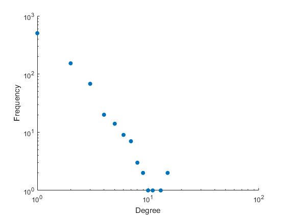
(a) Ito-core

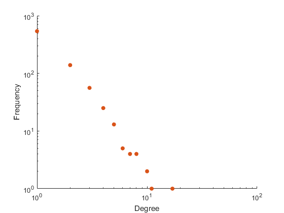
(b) Uetz-screen

Figure 5: Empirical degree distributions for S. cerevisiae PIN on log-log scale.

Figure 5 displays the empirical degree distributions of the Ito-core (Ito et al.,, 2001) and Uetz-screen (Uetz et al.,, 2000) Y2H assays of the S. cerevisiae PIN. When plotted on a log-log scale, these exhibit the characteristic straight line of a scale-free distribution. However, caution must be taken as these data sets constitute samples of size 813 and 437 proteins respectively from an estimated proteome size of 6000 (Goffeau et al.,, 1996). Stumpf et al., (2005) and Stumpf and Wiuf, (2005) show that subgraphs of scale-free networks are not scale-free, so the apparent power law distributions in figure 5 do not offer compelling evidence that the yeast PIN is scale-free. Further compounding the problem of making inferences from Y2H samples is the prevalence of false positives and false negatives, with false negative rates being as high as 90% (Hart et al.,, 2006; Ito et al.,, 2002). Han et al., (2005) show via simulation study that when measurement error is introduced, graphs with Erdős-Rényi, scale-free, and exponential distributions can lead to sampled subgraphs whose degree distributions are practically indistinguishable from one another. In what follows we consider conducting inference on the yeast PIN explicitly accounting for the sampling and false negative rates.

5.3 Data

We consider five data sets on the S. cerevisiae PIN taken from Yu et al., (2008), available for download from the Center for Cancer Systems Biology yeast interactome database. This includes the two sets displayed in figure 5: Ito-core (Ito et al.,, 2001), consisting of 843 interactions between 813 proteins; and Uetz-screen (Uetz et al.,, 2000), with 682 interactions between 806 proteins. Yu et al., (2008) test the quality of these data sets by comparing them to two independent assays and find that both data sets exhibit high specificity, with the interactions detected likely to be true positives, but low sensitivity. Yu et al., (2008) also construct three additional data sets: a binary gold standard (Binary-GS) set of 1,318 high-confidence interactions on 1,090 proteins; the CCSB-YI1 set consisting of 1,809 interactions among 1,278 proteins with specificity at least 94%; and Y2H-Union, which is the union of Ito-core, Uetz-screen, and CCSB-YI1. Y2H-Union is estimated to be 20% sensitive.

5.4 Method and Results

Data Set Test Family False Negative Rate 70% 80% 90% $\hat{\theta}$ P-value $\hat{\theta}$ P-value $\hat{\theta}$ P-value Ito-core Poisson 19.39 0.00 29.31 0.00 59.03 0.00 Scale-free 1.74 0.18 1.61 0.48 1.29 0.18 Exponential 0.07 0.05 0.05 0.07 0.02 0.04 Uetz-screen Poisson 16.30 0.00 24.67 0.00 49.75 0.00 Scale-free 1.80 0.49 1.68 0.87 1.39 0.49 Exponential 0.08 0.11 0.05 0.11 0.03 0.06 CCSB-YI1 Poisson 13.51 0.00 20.36 0.00 40.90 0.00 Scale-free 1.62 0.31 1.50 0.65 1.31 0.00 Exponential 0.07 0.00 0.05 0.00 0.03 0.00 Binary-GS Poisson 28.03 0.00 42.22 0.00 84.77 0.00 Scale-free 1.59 0.00 1.39 0.00 0.84 0.02 Exponential 0.05 0.02 0.03 0.03 0.01 0.01 Y2H-Union Poisson 11.07 0.00 16.68 0.00 33.47 0.00 Scale-free 1.72 0.00 1.58 0.00 1.35 0.17 Exponential 0.09 0.00 0.06 0.00 0.03 0.00

Table 3: Parameter estimates and p-values corresponding to the hypothesis test for each data set belonging to a poisson, scale-free, and exponential family of distributions respectively. Each test is conducted assuming false negative rates of 70%, 80%, and 90% respectively, with 500 bootstrap samples.

First we must address the distortion to the degree distribution imposed by sampling an induced subgraph with the possibility of false negatives. For simplicity we will assume that vertices are chosen through Bernoulli sampling, in which each vertex is included in the sample independently with probability $p$. Assume further that for any edge present in the population graph, that edge may only be observed in an induced subgraph independently with probability $r$. Thus if we consider a vertex in the sample with $k$ edges in the population, the probability it has $i$ edges in the induced subgraph is $Binom(rp,k)$. For small $rp$ this may be well approximated as $Poiss(rpk)$. Therefore we construct the design matrix in equation 2 such that its columns are poisson.

$$\mathbf{X}_{i,k+1}=\frac{e^{-rpk}(rpk)^{i}}{i!}\quad k=0,\dots,n-1$$ (11)

Following (Goffeau et al.,, 1996) we set $N=6,000$ to be the size of the yeast proteome. We set $p=\frac{n}{N}$, where $n$ is the sample size of the corresponding data set. We consider false negative rates of 70%, 80%, and 90%, corresponding to $r\in\{.3,.2,.1\}$. For each data set and false negative rate, we test three hypotheses: that the data were drawn from a graph whose degree distribution is poisson, $P_{G}(k;\theta)\propto\theta^{k}$; a graph whose degree distribution is scale-free, $P_{G}(k;\theta)\propto k^{-\theta}$; and a graph whose degree distribution is exponential, $P_{G}(k;\theta)\propto e^{-\theta k}$. Each test is performed at the 5% significance level with $B=500$ bootstrap samples.

Adjacency matrices for the sample graphs were constructed using data from the CCSB interactome database mentioned above. Self-loops have been removed such that each graph is simple and undirected. The data do not contain information on the number of isolate vertices measured. As such, our estimation procedure and bootstrap have been modified to mimic this by removing isolates from consideration.

Table 3 displays the results. The immediate result is that for each data set and each false negative rate, the hypothesis that the yeast PIN follows a poisson distribution is unanimously rejected. For Ito-core and Uetz-screen, only the scale-free hypothesis is retained. Scale-free is the only hypothesis retained for the CCSB-YI1 data set, except for at a false negative rate of 90% for which all hypotheses are rejected. Y2H-Union rejects all hypotheses except for scale-free at the 90% false negative rate. This is seems odd considering Y2H-Union is the combination of Ito-core, Uetz-screen, and CCSB-YI1; all of which are unable to reject at the 70% and 80% false negative levels. Binary-GS is especially odd, only retaining the exponential family for the 70% and 80% rates while switching to only retain scale-free at the 90% rate. The fact that the parameter estimates for the Binary-GS data set is far out of line with those of the other sets suggests this may be an artifact of how the data were aggregated.

These results need to be taken with a grain of salt. It is not necessarily true that the sampling methodology may be well approximated by random sampling of proteins within the S. cerevisiae proteome. Further the rates of false positives and negatives are not known with precision. What we do glean from these results is that the Erdős-Rényi random graph model, resulting in poisson degree distributions, is not a good candidate for the degree distribution of the S. cerevisiae protein interaction network.

6 Discussion

We have proposed a procedure for conducting
goodness-of-fit tests for sampled subgraphs. The procedure relies on a parametric bootstrap being adapted to mimic the subgraph sampling process. A monte carlo study reveals that this test posesses good size properties, keeping the type I error rate close to the specified nominal level, while having good power in a large region of the parameter space. In this paper we have focused on a sampling design where a subset of vertices are selected, either by Bernoulli or simple random sampling, and the subgraph induced by those vertices constitutes our sample; though this is not the only sampling design servicable by our methodology. It applies to any sampling design where the distortion to the degree distribution may be modelled as a linear transformation, as in equation 2, where the matrix $\mathbf{X}$ does not depend on features of the graph being sampled. Incident edge, traceroute, snowball, and ego sampling are all included in this subset.

A possible impediment to the utility of this approach is that for the bootstrap to function, a graph on $N$ vertices must be constructed, where $N$ is the number of vertices in the population. For large online social networks, which can contain millions of vertices and edges, storage of the corresponding adjacency matrix, and the time required to sample subgraphs from it, may be too burdensome. An efficienct implementation of the bootstrap for such large graphs presents an area for future research.

References

- Albert and Barabási, (2002) Albert, R. and Barabási, A.-L. (2002). Statistical mechanics of complex networks. Rev. Mod. Phys., 74:47–97.
- Albert et al., (2000) Albert, R., Jeong, H., and Barabási, A.-L. (2000). Error and attack tolerance of complex networks. Nature, 406(6794):378–382.
- Barabási and Albert, (1999) Barabási, A.-L. and Albert, R. (1999). Emergence of scaling in random networks. Science, 286(5439):509–512.
- Bender and Canfield, (1978) Bender, E. A. and Canfield, E. (1978). The asymptotic number of labeled graphs with given degree sequences. Journal of Combinatorial Theory, Series A, 24(3):296 – 307.
- Bollobás, (1982) Bollobás, B. (1982). The asymptotic number of unlabelled regular graphs. J. London Math. Soc, 26(2):201–206.
- Boss et al., (2004) Boss, M., Elsinger, H., Summer, M., and 4, S. T. (2004). Network topology of the interbank market. Quantitative Finance, 4(6):677–684.
- Doyle et al., (2005) Doyle, J. C., Alderson, D. L., Li, L., Low, S., Roughan, M., Shalunov, S., Tanaka, R., and Willinger, W. (2005). The “robust yet fragile” nature of the internet. Proceedings of the National Academy of Sciences of the United States of America, 102(41):14497–14502.
- Efron, (1979) Efron, B. (1979). Bootstrap methods: Another look at the jackknife. Ann. Statist., 7(1):1–26.
- Eldar, (2009) Eldar, Y. C. (2009). Generalized sure for exponential families: Applications to regularization. IEEE Transactions on Signal Processing, 57(2):471–481.
- Erdos and Rényi, (1960) Erdos, P. and Rényi, A. (1960). On the evolution of random graphs. Publ. Math. Inst. Hung. Acad. Sci, 5(1):17–60.
- Fields and Song, (1989) Fields, S. and Song, O.-k. (1989). A novel genetic system to detect protein–protein interactions. Nature, 340(6230):245–246.
- Frank, (1980) Frank, O. (1980). Estimation of the number of vertices of different degrees in a graph. Journal of Statistical Planning and Inference, 40(1):45 – 50.
- Gai et al., (2011) Gai, P., Haldane, A., and Kapadia, S. (2011). Complexity, concentration and contagion. Journal of Monetary Economics, 58(5):453 – 470. Carnegie-Rochester Conference on public policy: Normalizing Central Bank Practice in Light of the credit Turmoi, 12–13 November 2010.
- Goffeau et al., (1996) Goffeau, A., Barrell, B. G., Bussey, H., Davis, R., Dujon, B., Feldmann, H., Galibert, F., Hoheisel, J., Jacq, C., Johnston, M., et al. (1996). Life with 6000 genes. Science, 274(5287):546–567.
- Goldstein et al., (2004) Goldstein, M. L., Morris, S. A., and Yen, G. G. (2004). Problems with fitting to the power-law distribution. The European Physical Journal B - Condensed Matter and Complex Systems, 41(2):255–258.
- Han et al., (2005) Han, J.-D. J., Dupuy, D., Bertin, N., Cusick, M. E., and Vidal, M. (2005). Effect of sampling on topology predictions of protein-protein interaction networks. Nature biotechnology, 23(7):839.
- Hart et al., (2006) Hart, G. T., Ramani, A. K., and Marcotte, E. M. (2006). How complete are current yeast and human protein-interaction networks? Genome biology, 7(11):120.
- Ito et al., (2001) Ito, T., Chiba, T., Ozawa, R., Yoshida, M., Hattori, M., and Sakaki, Y. (2001). A comprehensive two-hybrid analysis to explore the yeast protein interactome. Proceedings of the National Academy of Sciences, 98(8):4569–4574.
- Ito et al., (2002) Ito, T., Ota, K., Kubota, H., Yamaguchi, Y., Chiba, T., Sakuraba, K., and Yoshida, M. (2002). Roles for the two-hybrid system in exploration of the yeast protein interactome. Molecular & Cellular Proteomics, 1(8):561–566.
- Jeong et al., (2001) Jeong, H., Mason, S. P., Barabasi, A.-L., and Oltvai, Z. N. (2001). Lethality and centrality in protein networks. Nature, 411(6833):41–42.
- Kolaczyk, (2009) Kolaczyk, E. D. (2009). Sampling and Estimation in Network Graphs, pages 1–30. Springer New York, New York, NY.
- Lilliefors, (1967) Lilliefors, H. W. (1967). On the kolmogorov-smirnov test for normality with mean and variance unknown. Journal of the American Statistical Association, 62(318):399–402.
- Lilliefors, (1969) Lilliefors, H. W. (1969). On the kolmogorov-smirnov test for the exponential distribution with mean unknown. Journal of the American Statistical Association, 64(325):387–389.
- Massey Jr, (1951) Massey Jr, F. J. (1951). The kolmogorov-smirnov test for goodness of fit. Journal of the American statistical Association, 46(253):68–78.
- Newman et al., (2001) Newman, M. E. J., Strogatz, S. H., and Watts, D. J. (2001). Random graphs with arbitrary degree distributions and their applications. Phys. Rev. E, 64:026118.
- Pearson, (1900) Pearson, K. (1900). X. on the criterion that a given system of deviations from the probable in the case of a correlated system of variables is such that it can be reasonably supposed to have arisen from random sampling. The London, Edinburgh, and Dublin Philosophical Magazine and Journal of Science, 50(302):157–175.
- Ramani et al., (2008) Ramani, S., Blu, T., and Unser, M. (2008). Monte-carlo sure: A black-box optimization of regularization parameters for general denoising algorithms. IEEE Transactions on Image Processing, 17(9):1540–1554.
- Ross-Macdonald et al., (1999) Ross-Macdonald, P., Coelho, P. S. R., Roemer, T., Agarwal, S., Kumar, A., Jansen, R., Cheung, K.-H., Sheehan, A., Symoniatis, D., Umansky, L., Heidtman, M., Nelson, F. K., Iwasaki, H., Hager, K., Gerstein, M., Miller, P., Roeder, G. S., and Snyder, M. (1999). Large-scale analysis of the yeast genome by transposon tagging and gene disruption. Nature, 402(6760):413–418.
- Stein, (1981) Stein, C. M. (1981). Estimation of the mean of a multivariate normal distribution. The Annals of Statistics, 9(6):1135–1151.
- Stumpf and Wiuf, (2005) Stumpf, M. P. and Wiuf, C. (2005). Sampling properties of random graphs: the degree distribution. Physical Review E, 72(3):036118.
- Stumpf et al., (2005) Stumpf, M. P., Wiuf, C., and May, R. M. (2005). Subnets of scale-free networks are not scale-free: sampling properties of networks. Proceedings of the National Academy of Sciences of the United States of America, 102(12):4221–4224.
- Tibshirani, (1996) Tibshirani, R. (1996). Regression shrinkage and selection via the lasso. Journal of the Royal Statistical Society. Series B (Methodological), 58(1):267–288.
- Uetz et al., (2000) Uetz, P., Giot, L., Cagney, G., Mansfield, T. A., et al. (2000). A comprehensive analysis of protein-protein interactions in saccharomyces cerevisiae. Nature, 403(6770):623.
- Vogelstein et al., (2000) Vogelstein, B., Lane, D., and Levine, A. J. (2000). Surfing the p53 network. Nature, 408(6810):307–310.
- Wald, (1943) Wald, A. (1943). Tests of statistical hypotheses concerning several parameters when the number of observations is large. Transactions of the American Mathematical society, 54(3):426–482.
- Winzeler et al., (1999) Winzeler, E. A., Shoemaker, D. D., Astromoff, A., Liang, H., Anderson, K., Andre, B., Bangham, R., Benito, R., Boeke, J. D., Bussey, H., Chu, A. M., Connelly, C., Davis, K., Dietrich, F., Dow, S. W., El Bakkoury, M., Foury, F., Friend, S. H., Gentalen, E., Giaever, G., Hegemann, J. H., Jones, T., Laub, M., Liao, H., Liebundguth, N., Lockhart, D. J., Lucau-Danila, A., Lussier, M., M’Rabet, N., Menard, P., Mittmann, M., Pai, C., Rebischung, C., Revuelta, J. L., Riles, L., Roberts, C. J., Ross-MacDonald, P., Scherens, B., Snyder, M., Sookhai-Mahadeo, S., Storms, R. K., Véronneau, S., Voet, M., Volckaert, G., Ward, T. R., Wysocki, R., Yen, G. S., Yu, K., Zimmermann, K., Philippsen, P., Johnston, M., and Davis, R. W. (1999). Functional characterization of the s. cerevisiae genome by gene deletion and parallel analysis. Science, 285(5429):901–906.
- Yu et al., (2008) Yu, H., Braun, P., Yıldırım, M. A., Lemmens, I., Venkatesan, K., Sahalie, J., Hirozane-Kishikawa, T., Gebreab, F., Li, N., Simonis, N., et al. (2008). High-quality binary protein interaction map of the yeast interactome network. Science, 322(5898):104–110.
- Zhang et al., (2015) Zhang, Y., Kolaczyk, E. D., and Spencer, B. D. (2015). Estimating network degree distributions under sampling: An inverse problem, with applications to monitoring social media networks. Ann. Appl. Stat., 9(1):166–199.