Dynamics of a quasiparticle in the $\alpha$-T₃ model: Role of pseudospin polarization and transverse magnetic field on zitterbewegung

Abstract

We consider the $\alpha$-$T_{3}$ model which provides a smooth crossover between the honeycomb lattice with pseudospin $1/2$ and the dice lattice with pseudospin $1$ through the variation of a parameter $\alpha$. We study the dynamics of a wave packet representing a quasiparticle in the $\alpha$-T₃ model with zero and finite transverse magnetic field. For zero field, it is shown that the wave packet undergoes a transient $zitterbewegung$ (ZB). Various features of ZB depending on the initial pseudospin polarization of the wave packet have been revealed. For an intermediate value of the parameter $\alpha$ i.e. for $0<\alpha<1$ the resulting ZB consists of two distinct frequencies when the wave packet was located initially in $rim$ site. However, the wave packet exhibits single frequency ZB for $\alpha=0$ and $\alpha=1$. It is also unveiled that the frequency of ZB corresponding to $\alpha=1$ gets exactly half of that corresponding to the $\alpha=0$ case. On the other hand, when the initial wave packet was in $hub$ site, the ZB consists of only one frequency for all values of $\alpha$. Using stationary phase approximation we find analytical expression of velocity average which can be used to extract the associated timescale over which the transient nature of ZB persists. On the contrary the wave packet undergoes permanent ZB in presence of a transverse magnetic field. Due to the presence of large number of Landau energy levels the oscillations in ZB appear to be much more complicated. The oscillation pattern depends significantly on the initial pseudospin polarization of the wave packet. Furthermore, it is revealed that the number of the frequency components involved in ZB depends on the parameter $\alpha$.

I Introduction

The conception $zitterbewegung$ (ZB) stands for an outlandish quantum motion, of a Dirac particle in vacuum, having length scale of the order of Compton wave length. It was originally envisioned by Schrödinger in 1930Schro . The main obstruction to establish the existence of ZB in vacuum experimentally is its ultra-short length scale. However, a ray of hope was shown in 2005 when Zawadkizawadki argued that a narrow gap semiconductor not only can host the intriguing phenomenon ZB but also the associated length scale can be enhanced up to five orders higher than that in vacuum. As a result, subsequent years witnessed immense interest in ZB in numerous systemszbgen including spin-orbit coupled two dimensional (2D) electron/hole gasesjohn ; zb2d1 ; zb2d2 ; zb2d3 ; zb2d4 ; zb2d5 ; zb2dH ; zb2dH2 , superconductorszbsup , sonic crystalzbsonic , photonic crystalzbphoton ; zbopp , carbon nanotubezbcnt , graphenezbgrph1 ; zbgrph2 ; zbgrph3 ; zbgrph4 ; zbgrph5 , other Dirac materialszbtopo ; zbMos2 ; zbMos22 and ultra-cold atomic gaseszbbec1 ; zbbec2 ; zbbec3 ; zbbec4 .

There exists several understandings behind the cause of ZB. It is believed that ZB happens as an outcome of the interference between positive and negative energy solutions of the Dirac equation. Huanghuang put forward a theory to establish a connection between ZB and electron’s intrinsic magnetic dipole moment. Later, Schliemannzb2d2 $et$ $al$ interpreted that ZB in a quantum well occurs as a consequence of spin rotation due to spin-orbit interaction (SOI). It is also mentionedzbbec1 that the ZB can be interpreted as a measurable aftermath of Berry phase in momentum space. Moreover, for a multiband quantum system, an explicit relation between Berry curvature and amplitude of ZB was also establishedzbCsr .

In general ZB has permanent character i.e. oscillations do not die out in time. When an electron is illustrated by a wave packet the resulting ZB undergoes a transient nature according to Locklock . It is also proposed recentlyzb2d5 that the permanent behavior of ZB in a spin-orbit coupled 2D electron gas can be restored by considering a time dependent Rashba SOI.

Furthermore, an intriguing quantum transport related phenomenon such as minimal conductivityZbKats of graphene was understood in the light of ZB. Very recently, Iwasaki et al ZbIwa demonstrated experimentally that conductance fluctuations in InAs quantum wells occur as a possible consequence of ZB.

From the perspective of ZB, most of the studies in electronic systems are mainly concerned about the ZB of quasiparticles with spin/pseudospin $S=1/2$. However, there exists an example which portrays ZB of spin-1 ultra-cold atomzbbec2 . To the best of our knowledge no such example of ZB of a quasiparticle with spin/pseudospin beyond $S=1/2$ exists in typical condensed matter systems. Hence, in this article we consider the ZB effect in a relatively new model named as $\alpha$-T₃ model in which quasiparticles are characterized by an enlarged pseudospin $S\geq 1/2$. The sole motivation behind adopting this model is due to growing interest in systems which are described by the generalized Dirac-Weyl equation with arbitrary pseudospin $S$ dice_S1 ; dice_S2 ; dice_S3 . Via the variation of a parameter $\alpha$, the $\alpha$-T₃ model reveals a smooth changeover from graphene ($\alpha=0$) to dice or T₃ lattice ($\alpha=1$). There has been a lot of studies in T₃ lattice from the standpoint of topological localization dice1 ; dice2 , magnetic frustration frust1 ; frust2 , Klein tunneling dice_Klein , minimal conductivityminT3 , plasmonplasm etc. Moreover, the existence of the $T_{3}$-model within the framework of optical latticedice_opt and semiconductor structuredice_grow is also predicted recently. In addition, the interest in $\alpha$-$T_{3}$ modeldice_alph is growing rapidly nowadays. According to Malcolm and Nicol dice_alph2 a Hg_1-xCd_xTe quantum well can be considered as $\alpha$-T₃ model with $\alpha=1/\sqrt{3}$ at a particular doping. The connection of the parameter $\alpha$ with the Berry phase makes the $\alpha$-T₃ model more interesting. In recent years, a number of studies have been performed on this model within the context of orbital magnetic responsedice_alph , magneto-transportdice_MagTr , optical conductivitydice_Berry ; dice_MagOP1 ; dice_MagOP2 , quantum tunnelingdice_QT , Wiess oscillationsdice_Wiess etc.

In this work we have investigated the problem of ZB of a quasiparticle in $\alpha$-T₃ model. We choose an initial Gaussian wave packet with definite pseudospin polarization to represent a quasiparticle. For $0<\alpha<1$, the quasiparticle undergoes ZB which is transient in nature and consists of two frequencies, namely, $2\Omega_{q}$ and $\Omega_{q}$. The interference between conduction and valence band leads to occur ZB with frequency $2\Omega_{q}$ whereas the $\Omega_{q}$-frequency ZB occurs as a result of interference between either conduction and flat band or flat and valence band. The nature of ZB depends significantly on the type of the initial pseudospin polarization. Particularly, when the initial pseudospin polarization was along $z$-direction, various interesting features of ZB emerge. For example, when the initial wave packet was concentrated entirely in any of the $rim$ sites the resulting ZB has two above mentioned frequencies for a finite $\alpha$. In this case we reveal a transition from $2\Omega_{q}$-frequency ZB to $\Omega_{q}$-frequency ZB as $\alpha$ is tuned from $0$ to $1$. When the wave packet was located initially in the $hub$ site, the resulting ZB has only one frequency $2\Omega_{q}$ for all possible values of $\alpha$. In the limit of large width of wave packet we obtain analytical expression for the expectation value of velocity operator from which one can extract the timescale over which the ZB dies out. We also consider the effect of other possible pseudospin polarization on ZB. In addition we incorporate the effect of an external quantizing magnetic field on the ZB. In this case the temporal behavior of ZB is permanent. The effect of different pseudospin polarization has also been discussed. Using Fourier transformation we obtain frequency components involved in ZB for a particular choice of pseudospin polarization. We also find that the number of frequencies present in ZB depends significantly on the parameter $\alpha$.

Rest of the present paper is organized in the following fashion. In section II, we discuss zero field ZB by incorporating the basic informations about physical system, time evolution of wave packet, and rigorous calculations of the expectation values of physical observables. The effect of perpendicular magnetic field on ZB is considered in section III. We summarize the obtained results in section IV.

II In absence of magnetic field

II.1 Lattice structure and low lying energy states

As depicted in Fig. 1(a), $\alpha$-T₃ model has honeycomb lattice structure with an additional site at the center of each hexagon. Each unit cell (shown by the dashed rhombus) contains $3$ sites. With respect to the co-ordination number (CN), those sites are classified into two categories, namely $rim$ and $hub$ sites. As evident from Fig. 1(a) sites B and C are both $rim$ sites having CN $3$ whereas site A is known as $hub$ site with CN $6$. Note that each nearest-neighbor pair consists of one $rim$ and one $hub$ sites. The sites A and B are connected through hopping parameter $t$ while hopping energy between A and C is $\alpha t$.

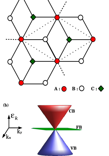
Figure 1: (a) The lattice structure of a $\alpha$-T₃ model. Here, A(denoted by filled circle) is the hub site while B(denoted by empty circle) and C(denoted by solid square) are rim sites. The hopping energy between A and B is $t$ whereas the hopping energy between A and C is $\alpha t$. The dotted rhombus denotes the unit cell. The dashed lines emerging from A sites indicate that each A site is connected to the next C site. (b) The energy surfaces are drawn as a function of wave vector ${\bf k}$ in arbitrary units. The zero energy FB lies in the ($k_{x},k_{y}$) plane whereas other bands exhibit linear dispersion with ${\bf k}$.

The low energy excitations near the Dirac point in a particular valley are described by the following Hamiltoniandice_alph

$$H({\bf p})=\begin{pmatrix}0&f_{\bf p}\cos\varphi&0\\ f_{\bf p}^{\ast}\cos\varphi&0&f_{\bf p}\sin\varphi\\ 0&f_{\bf p}^{\ast}\sin\varphi&0\end{pmatrix},$$ (1)

where $f_{\bf p}=v_{F}(\zeta p_{x}-ip_{y})$ with $v_{F}$ being the Fermi velocity. The valley index $\zeta$ takes a value $+1(-1)$ for ${\rm K}({\rm K}^{\prime})$ valley. Finally, following relation $\alpha=\tan\varphi$ holds between $\alpha$ and $\varphi$. The energy spectrum corresponding to the Hamiltonian given in Eq. (1) consists of three branches. Out of them two are linearly dispersing $\varepsilon_{\bf k}^{\lambda}=\lambda\hbar v_{F}k$ with $\lambda=\pm 1$ and $k=|{\bf p}|/\hbar$, known as conic band. The conic band itself consists of conduction band (CB) and valence band (VB) corresponding to $\lambda=+1$ and $\lambda=-1$, respectively. The other energy branch is dispersionless and is known as flat band (FB). All these energy branches are depicted in Fig.1(b). The wave functions corresponding to conic band and FB around the ${\rm K}$-valley are, respectively, given by

$$\psi_{\bf k}^{\lambda}({\bf r})=\frac{1}{\sqrt{2}}\left(\begin{array}[]{c}\cos\varphi\,e^{-i\theta}\\ \lambda\\ \sin\varphi\,e^{i\theta}\end{array}\right)\frac{e^{i{{\bf k}\cdot{\bf r}}}}{2\pi}$$ (5)

and

$$\psi_{\bf k}^{0}({\bf r})=\frac{1}{\sqrt{2}}\left(\begin{array}[]{c}\sin\varphi\,e^{-i\theta}\\ 0\\ -\cos\varphi\,e^{i\theta}\end{array}\right)\frac{e^{i{{\bf k}\cdot{\bf r}}}}{2\pi},$$ (9)

where $\theta$ is the polar angle of the wave vector ${\bf k}$.

II.2 Velocity and pseudospin operators

From Eq. (1), using the relation $v_{i}=\partial{H}/\partial{p_{i}}$ with $i=x,y$, one can obtain the following components of the velocity matrix for the ${\rm K}$-valley as

$$v_{x}=v_{F}\begin{pmatrix}0&\cos\phi&0\\ \cos\phi&0&\sin\phi\\ 0&\sin\phi&0\end{pmatrix}$$ (10)

and

$$v_{y}=v_{F}\begin{pmatrix}0&-i\cos\phi&0\\ i\cos\phi&0&-i\sin\phi\\ 0&i\sin\phi&0\end{pmatrix}.$$ (11)

The $x$ and $y$ components of the pseudospin operator are governed from the velocity operators as $S_{i}=\hbar v_{i}/v_{F}$ with $i=x,y$. The $z$-component of ${\bf S}$ is obtained through the commutation relation $[S_{x},S_{y}]=i\hbar S_{z}$ as

$$S_{z}=2\hbar\begin{pmatrix}\cos^{2}\phi&0&0\\ 0&-\cos(2\phi)&0\\ 0&0&-\sin^{2}\phi\end{pmatrix}.$$ (12)

II.3 Time evolution of a initial wave packet

To study the dynamics of a quasiparticle, it is important to know the corresponding wave function at a later time $t$. In the following, we consider the initial wave function representing the quasiparticle to be a plane wave modulated by a Gaussian wave packet

$$\Psi({\bf r},0)=\frac{1}{2\pi C}\int d{\bf k}\,a({\bf k},0)e^{i{\bf k}\cdot{\bf r}}\begin{pmatrix}c_{1}\\ c_{2}\\ c_{3}\end{pmatrix},$$ (13)

where the wave packet $a({\bf k},0)=(d/\sqrt{\pi})e^{-d^{2}({\bf k}-{\bf k_{0}})^{2}/2}$ is centered at some wave vector ${\bf k}={\bf k_{0}}$ and $d$ is its width. Note that the wave packet was polarized initially along any arbitrary direction characterized by the constants $c_{1}$, $c_{2}$, and $c_{3}$ which are, in general, complex numbers. The normalization constant $C$ is defined as $C=\sqrt{|c_{1}|^{2}+|c_{2}|^{2}+|c_{3}|^{2}}$. The wave function, at a later time $t$, can be obtained by applying appropriate time evolution operator onto $\Psi({\bf r},0)$. We find the time evolved state as

$$\Psi({\bf r},t)=\frac{1}{2\pi}\int d{\bf k}\,a({\bf k},0)e^{i{\bf k}\cdot{\bf r}}\begin{pmatrix}\kappa_{1}({\bf k},t)\\ \kappa_{2}({\bf k},t)\\ \kappa_{3}({\bf k},t)\end{pmatrix},$$ (14)

where $\kappa_{\mu}({\bf k},t)$’s, with $\mu=1,2,3$, are obtained from the following matrix equation

$$\begin{pmatrix}\kappa_{1}({\bf k},t)\\ \kappa_{2}({\bf k},t)\\ \kappa_{3}({\bf k},t)\end{pmatrix}=\frac{1}{C}\begin{pmatrix}\sin^{2}\varphi+\cos^{2}\varphi\cos(\Omega_{\bf k}t)&-i\cos\varphi\,e^{-i\theta}\sin(\Omega_{\bf k}t)&\sin\varphi\,\cos\varphi\,e^{-2i\theta}[\cos(\Omega_{\bf k}t)-1]\\ -i\cos\varphi\,e^{i\theta}\sin(\Omega_{\bf k}t))&\cos(\Omega_{\bf k}t)&-i\sin\varphi\,e^{-i\theta}\sin(\Omega_{\bf k}t)\\ \sin\varphi\,\cos\varphi\,e^{2i\theta}[\cos(\Omega_{\bf k}t)-1]&-i\sin\varphi\,e^{i\theta}\,\sin(\Omega_{\bf k}t)&\cos^{2}\varphi+\sin^{2}\varphi\,\cos(\Omega_{\bf k}t)\end{pmatrix}\begin{pmatrix}c_{1}\\ c_{2}\\ c_{3}\end{pmatrix}$$ (15)

It is noteworthy that Eq. (14) is the Fourier transformation of the following function

$$\Phi({\bf k},t)=a({\bf k},0)\begin{pmatrix}\kappa_{1}({\bf k},t)\\ \kappa_{2}({\bf k},t)\\ \kappa_{3}({\bf k},t)\end{pmatrix}.$$ (16)

Equation (16) represents the time evolved state in the momentum space which can be used to calculate the expectation values of various physical observables.

II.4 Expectation value of the velocity operator

The expectation value of a physical observable corresponding to an operator $\hat{O}$ is defined as $\langle\hat{O}(t)\rangle=\int d{\bf k}\Phi^{\dagger}({\bf k},t)\hat{O}\Phi({\bf k},t)$. Instead of evaluating the expectation value of position operator we prefer here to calculate that of velocity operator because the former is always obtained by integrating the later with suitable initial conditions.

Now the expectation values of the components of velocity operator can be obtained as

$$\langle v_{x}\rangle=2v_{F}\int d{\bf k}|a({\bf k},0)|^{2}{\rm Re}\big{(}\cos\varphi\,\kappa_{1}^{\ast}\kappa_{2}+\sin\varphi\,\kappa_{2}^{\ast}\kappa_{3}\big{)}$$ (17)

and

$$\langle v_{y}\rangle=2v_{F}\int d{\bf k}|a({\bf k},0)|^{2}{\rm Im}\big{(}\cos\varphi\,\kappa_{1}^{\ast}\kappa_{2}+\sin\varphi\,\kappa_{2}^{\ast}\kappa_{3}\big{)}.$$ (18)

By defining $\Sigma_{\mu\sigma}(t)=\int d{\bf k}|a({\bf k},0)|^{2}\kappa_{\mu}^{\ast}({\bf k},t)\kappa_{\sigma}({\bf k},t)$ with $\mu,\sigma=1,2,3$, Eqs. (17) and (18) can be further written in the following compact form

$$\begin{pmatrix}\langle v_{x}(t)\rangle\\ \langle v_{y}(t)\rangle\end{pmatrix}=2v_{F}\begin{pmatrix}{\rm Re}\\ {\rm Im}\end{pmatrix}\Big{(}\cos\varphi\Sigma_{12}(t)+\sin\varphi\Sigma_{23}(t)\Big{)}.$$ (19)

Without any loss of generality, we consider the initial wave packet was moving along +$x$ direction with wave vector ${\bf k_{0}}=k_{0}\hat{x}$. After doing the angular integration, we obtain $\Sigma_{12}(t)$ and $\Sigma_{23}(t)$ as

$$\Sigma_{12}(t)=\frac{2}{C^{2}}e^{-a^{2}}\int_{0}^{\infty}dq\,q\,e^{-q^{2}}\Bigg{[}\Big{\{}c_{1}^{\ast}c_{2}\sin^{2}\varphi I_{0}(2aq)-c_{3}^{\ast}c_{2}\sin\varphi\cos\varphi I_{2}(2aq)\Big{\}}\cos(\Omega_{q}t)$$ (20)

$$+ i\Big{\{}c_{3}^{\ast}c_{1}\sin\varphi\cos^{2}\varphi I_{3}(2aq)+\Big{(}\big{(}|c_{3}|^{2}-|c_{1}|^{2}\big{)}\sin^{2}\varphi\cos\varphi-c_{1}^{\ast}c_{3}\sin^{3}\varphi\Big{)}I_{1}(2aq)\Big{\}}\sin(\Omega_{q}t)$$

$$+ \Big{\{}c_{1}^{\ast}c_{2}\cos^{2}\varphi I_{0}(2aq)+c_{3}^{\ast}c_{2}\sin\varphi\cos\varphi I_{2}(2aq)\Big{\}}\cos^{2}(\Omega_{q}t)+\Big{\{}c_{2}^{\ast}c_{1}\cos^{2}\varphi I_{2}(2aq)+c_{2}^{\ast}c_{3}\sin\varphi\cos\varphi I_{0}(2aq)\Big{\}}\sin^{2}(\Omega_{q}t)\Big{\}}$$

$$+ \frac{i}{2}\Big{\{}\Big{(}|c_{2}|^{2}\cos\varphi-|c_{1}|^{2}\cos^{3}\varphi-c_{1}^{\ast}c_{3}\sin\varphi\cos^{2}\varphi-|c_{3}|^{2}\sin^{2}\varphi\cos\varphi\Big{)}I_{1}(2aq)-c_{3}^{\ast}c_{1}\sin\varphi\cos^{2}\varphi I_{3}(2aq)\Big{\}}\sin(2\Omega_{q}t)\Bigg{]}$$

and

$$\Sigma_{23}(t)=\frac{2}{C^{2}}e^{-a^{2}}\int_{0}^{\infty}dq\,q\,e^{-q^{2}}\Bigg{[}\Big{\{}c_{2}^{\ast}c_{3}\cos^{2}\varphi I_{0}(2aq)-c_{2}^{\ast}c_{1}\sin\varphi\cos\varphi I_{2}(2aq)\Big{\}}\cos(\Omega_{q}t)$$ (21)

$$+ i\Big{\{}-c_{3}^{\ast}c_{1}\sin^{2}\varphi\cos\varphi I_{3}(2aq)+\Big{(}\big{(}|c_{3}|^{2}-|c_{1}|^{2}\big{)}\sin\varphi\cos^{2}\varphi+c_{1}^{\ast}c_{3}\cos^{3}\varphi\Big{)}I_{1}(2aq)\Big{\}}\sin(\Omega_{q}t)$$

$$+ \Big{\{}c_{2}^{\ast}c_{3}\sin^{2}\varphi I_{0}(2aq)+c_{2}^{\ast}c_{1}\sin\varphi\cos\varphi I_{2}(2aq)\Big{\}}\cos^{2}(\Omega_{q}t)+\Big{\{}c_{3}^{\ast}c_{2}\sin^{2}\varphi I_{2}(2aq)+c_{1}^{\ast}c_{2}\sin\varphi\cos\varphi I_{0}(2aq)\Big{\}}\sin^{2}(\Omega_{q}t)\Big{\}}$$

$$+ \frac{i}{2}\Big{\{}\Big{(}|c_{3}|^{2}\sin^{3}\varphi-|c_{2}|^{2}\sin\varphi+c_{1}^{\ast}c_{3}\sin^{2}\varphi\cos\varphi+|c_{1}|^{2}\sin\varphi\cos^{2}\varphi\Big{)}I_{1}(2aq)+c_{3}^{\ast}c_{1}\sin^{2}\varphi\cos\varphi I_{3}(2aq)\Big{\}}\sin(2\Omega_{q}t)\Bigg{]},$$

where $a=k_{0}d$, $q=kd$, $\Omega_{q}=v_{F}q/d$, and $I_{\nu}(x)$ is the $\nu$-th order modified Bessel function of first kind. Note that in Eqs. (20) and (21) there exist two frequencies namely $\Omega_{q}$ and $2\Omega_{q}$. The former is a result of interference between either FB & VB or CB &FB while the latter arises due to the coupling between CB & VB.

II.5 Various types of pseudospin polarization

We are merely interested in the dynamics of the Gaussian wave packet of different types of initial pseudo-spin polarization. Here, we will discuss all the possibilities corresponding to various combinations of $c_{1}$, $c_{2}$, and $c_{3}$.

1.  z-polarization

Here, we consider the wave packet was polarized initially along $+z$ direction. In this case the possible combinations of $(c_{1},c_{2},c_{3})$ are $(1,0,0)$, $(0,1,0)$, and $(0,0,1)$ corresponding to the eigen states of $S_{z}$-operator. Physically for the choices $(1,0,0)$ and $(0,0,1)$ the initial wave function was concentrated solely in any of the $rim$ sites while the choice $(0,1,0)$ corresponds to the case in which the wave function was entirely located in the $hub$ site initially. Let us now discuss all the possibilities one by one.

(i) First we consider $c_{1}=1$, $c_{2}=0$, and $c_{3}=0$ i.e. the initial wave packet was located in the $rim$ site B only. From Eqs. (19), (20), and (21), after a straightforward calculation, we find $\langle v_{x}(t)\rangle=0$ whereas $\langle v_{y}(t)\rangle$ takes the following form

$$\langle v_{y}(t)\rangle= - 2v_{F}\cos^{2}\varphi e^{-a^{2}}\int dqqe^{-q^{2}}I_{1}(2aq)\Big{[}\cos(2\varphi)$$ (22)

$$\times \sin(2q\tau)+2\Big{\{}1-\cos(2\varphi)\Big{\}}\sin(q\tau)\Big{]},$$

where $\tau=v_{F}t/d$. Note that Eq. (22) is an example of two-frequency ZB for a finite $\alpha$. The interference between CB and VB leads to the first term in the square bracket in Eq. (22) while the second term is appeared as a consequence of the interference between either CB and FB or VB and FB. When $\alpha=0$ i.e. $\varphi=0$ the second term in the square bracket of Eq. (22) contributes nothing to $\langle v_{y}(t)\rangle$. In this case the velocity average exhibits single frequency ZB determined from the interference between CB and VB which basically reminiscences the case of graphene. In the opposite limit i.e. for $\alpha=1$ we have $\varphi=\pi/4$. In this case, Eq. (22) retains only the second term in square bracket. Here, $\langle v_{y}(t)\rangle$ performs single frequency ZB, determined from the coupling between either CB and FB or FB and VB. In other words, for $\alpha=1$, the interference between CB and VB is completely prevented by FB.

The expectation value of position operator is obtained by integrating Eq. (22) with the initial condition: $\langle y(t)\rangle=0$ at $t=0$. Evaluating the $q$-integral in Eq. (22) numerically for $a=5$, we show the behavior of $\langle v_{y}(t)\rangle$ and $\langle y(t)\rangle$ in Fig. 2 and Fig. 3, respectively for different values of $\alpha$.

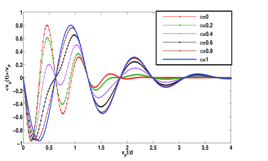
Figure 2: Time dependence of the expectation value of velocity operator for $a$=$5$. We consider initial pseudospin polarization along $z$-direction with components $c_{1}$=$1$, $c_{2}$=$0$, and $c_{3}$=$0$.

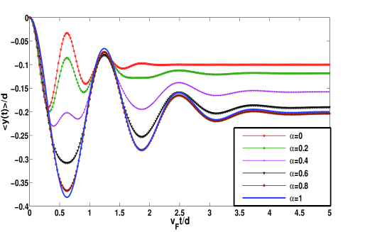
Figure 3: Time dependence of the expectation value of position operator for $a$=$5$. We consider initial pseudospin polarization along $z$-direction with components $c_{1}$=$1$, $c_{2}$=$0$, and $c_{3}$=$0$.

Both figures clearly demonstrate a crossover from a ZB of frequency $2\Omega_{q}$ to a ZB of frequency $\Omega_{q}$ with the smooth evolution of $\alpha$ from $0$ to $1$. In other words, as $\alpha$ approaches $1$, the frequency of ZB gets reduced to half of the value corresponding to $\alpha=0$. It is difficult to comment on the frequency of ZB for $0<\alpha<1$. Due to the interplay of two frequencies, namely, $2\Omega_{q}$ and $\Omega_{q}$ a complicated pattern is obtained for $\alpha=0.4$. It is worthy to notice that only one frequency either $2\Omega_{q}$ or $\Omega_{q}$ roughly dominates when $\alpha$ is below or above the value $\alpha=0.4$. As evident from Fig. 2 and Fig. 3, the resultant ZB is transient in character. To understand this transient behavior, it is possible to find an approximate analytical expression of Eq. (22) when the width of the wave packet is large enough i.e. for $a\gg 1$. In this limit the modified Bessel function $I_{1}(2aq)$ can be approximated as $I_{1}(2aq)\approx e^{2aq}/\sqrt{4\pi aq}$. With the help of the stationary phase approximation we obtain

$$\langle v_{y}(t)\rangle\approx - \frac{v_{F}}{2}\cos^{2}\varphi\Big{[}\cos(2\varphi)e^{-\tau^{2}}\sin(2a\tau)$$ (23)

$$+ 2\big{\{}1-\cos(2\varphi)\big{\}}e^{-\tau^{2}/4}\sin(a\tau)\Big{]}.$$

Note that the presence of decaying exponential terms in Eq. (23) clearly explains the transient behavior of ZB. For $\alpha=0$ the ZB decays rapidly due to the presence of the term $e^{-\tau^{2}}$ in Eq. (23). Here, the characteristic time scale corresponding to the decay in ZB amplitude is of the order of $d/v_{F}$. When $\alpha=1$ ZB decays slowly in comparison to the $\alpha=0$. This behavior is justified by the presence of $e^{-\tau^{2}/4}$ term in Eq. (23). Here the characteristic decay time scale is $2d/v_{F}$. It is also evident from Fig. 2 and 3, the second term within the square bracket in Eq. (23) dominates over the first term in the intermediate range of $\alpha$ i.e. $0<\alpha<1$.

(ii) Next, we consider another choice, namely, $c_{1}=0$, $c_{2}=0$, and $c_{3}=1$. In this case initially the electronic wave function was concentrated only in the other $rim$ site C. Here we find $\langle v_{x}(t)\rangle=0$ and

$$\langle v_{y}(t)\rangle= - 2v_{F}\sin^{2}\varphi e^{-a^{2}}\int dqqe^{-q^{2}}I_{1}(2aq)\Big{[}\cos(2\varphi)$$ (24)

$$\times \sin(2q\tau)-2\Big{\{}1+\cos(2\varphi)\Big{\}}\sin(q\tau)\Big{]}.$$

It is obvious from Eq. (24) that $\langle v_{y}(t)\rangle=0$ when $\alpha=0$. This clearly contradicts the established results corresponding to graphene. However, the discrepancy arose here is apparent because we are dealing with pseudospin-$1$. For graphene the pseudospin component $c_{3}$ is completely absent. Hence, the results corresponding to graphene can not be correctly interpreted from Eq. (24). For a finite $\alpha$, comparing Eq. (22) and Eq. (24), one may say that choices (i) and (ii) impose two-fold differences in ZB. Firstly, the amplitudes differ by a $\alpha$-dependent factor, namely, $\sin^{2}\varphi$ and $\cos^{2}\varphi$. Secondly, the second terms in the square brackets in Eq. (22) and (24) are different which may bring a phase difference in the oscillations. In the $a>>1$ limit, we obtain

$$\langle v_{y}(t)\rangle\approx - \frac{v_{F}}{2}\sin^{2}\varphi\Big{[}\cos(2\varphi)e^{-\tau^{2}}\sin(2a\tau)$$ (25)

$$- 2\big{\{}1+\cos(2\varphi)\big{\}}e^{-\tau^{2}/4}\sin(a\tau)\Big{]}.$$

(iii) Finally, we consider $c_{1}=0$, $c_{2}=1$, and $c_{3}=0$. The physical meaning of this particular choice corresponds to the initial localization of the wave function at the $hub$ site A. In this case, we obtain $\langle v_{x}(t)\rangle=0$ and

$$\langle v_{y}(t)\rangle=2v_{F}\cos(2\varphi)e^{-a^{2}}\int dqqe^{-q^{2}}I_{1}(2aq)\sin(2q\tau).$$ (26)

It is transparent from Eq. (26) that ZB consists of only one frequency governed by the energy difference between CB and VB for all values of $\alpha$. For this specific case, the FB contributes nothing to ZB. In the large $a$ limit, we find

$$\langle v_{y}(t)\rangle\approx \frac{v_{F}}{2}\cos(2\varphi)e^{-\tau^{2}}\sin(2a\tau).$$ (27)

For all the choices of $(c_{1},c_{2},c_{3})$, we obtain $\langle v_{x}(t)\rangle=0$ but $\langle v_{y}(t)\rangle\neq 0$. This implies that ZB occurs in a direction perpendicular to the direction of initial wave vector and pseudospin of the wave packet. Interestingly, we also note that the behavior of ZB is significantly dependent on the type of the initial pseudospin polarization of the wave packet. More specifically, when the initial wave packet was located entirely in any of the $rim$ sites, as understood from Eq. (22) and (24), corresponding ZB consists of two frequencies for $0<\alpha<1$. But when the initial wave packet was in the $hub$ site, we obtain single frequency ZB for all $\alpha$ as evident from Eq. (26). To establish all qualitative arguments made earlier we portray the time evolution of the expectation values of velocity and position operators in Fig. 4 for different choices of $(c_{1},c_{2},c_{3})$. For the plots we consider $\alpha=0.5$ and $a=5$. As illustrated in Fig. 4 the ZBs in position and velocity corresponding to different choices clearly differ in phase and amplitude. The ZB corresponding to the choice $(c_{1},c_{2},c_{3})=(0,1,0)$ decays more rapidly than the other choices due to the structure of the Eq. (27). Moreover, the ZB in position for $(c_{1},c_{2},c_{3})=(1,0,0)$ is negative while the ZBs for other choices are positive.

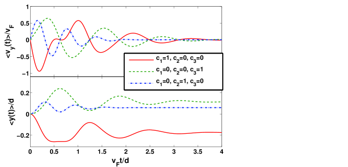
Figure 4: Time dependence of the expectation values of velocity and position operator for different choices of $(c_{1},c_{2},c_{3})$. Here, we consider $a=5$ and $\alpha=0.5$.

2.  x-polarization

Now, we seek to study the wave packet dynamics by considering that initial pseudospin polarization was in the $x$-direction. The operator $S_{x}$ has three eigenstates corresponding to the eigen values, namely, $0,\pm 1$(in units of $\hbar$). For those states we have following choices of $(c_{1},c_{2},c_{3})$, namely, $(\sin\varphi,0,-\cos\varphi)$, $(\cos\varphi,1,\sin\varphi)$, and $(-\cos\varphi,1,-\sin\varphi)$.

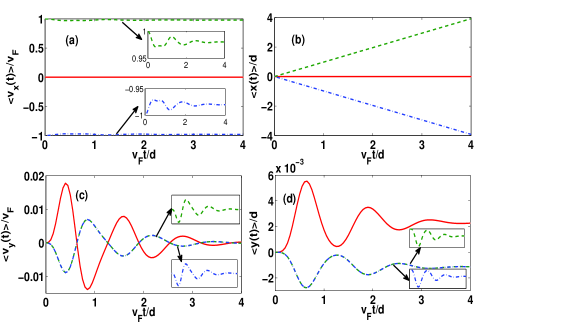
Figure 5: Time dependence of the expectation values of velocity and position operator when the initial pseudospin was polarized along $x$-direction. Here, solid(red), dashed(green), and dot-dashed(blue) lines correspond to different values of $(c_{1},c_{2},c_{3})$, namely, $(\sin\varphi,0,-\cos\varphi)$, $(\cos\varphi,1,\sin\varphi)$, and $(-\cos\varphi,1,-\sin\varphi)$, respectively. We also consider $a=5$ and $\alpha=0.5$.

In Fig. 5 the time dependence of the expectation values of position and velocity operators are shown corresponding to the above mentioned choices of $(c_{1},c_{2},c_{3})$ for a fixed $\alpha=0.5$. In contrast to the case 1, here both $\langle x(t)\rangle$ and $\langle v_{x}(t)\rangle$ do not vanish for all choices of $(c_{1},c_{2},c_{3})$. When $(c_{1},c_{2},c_{3})=(\sin\varphi,0,-\cos\varphi)$, both $\langle x(t)\rangle$ and $\langle v_{x}(t)\rangle$ are zero. Corresponding to the remaining choices of $(c_{1},c_{2},c_{3})$, namely, $(\cos\varphi,1,\sin\varphi)$, and $(-\cos\varphi,1,-\sin\varphi)$ both $\langle x(t)\rangle$ and $\langle v_{x}(t)\rangle$ are mirror image of each other individually. Although $\langle v_{x}(t)\rangle$ shows a tiny oscillation as depicted in the insets of Fig. 5(a) but $\langle x(t)\rangle$ exhibits a linear dependence with time (Fig. 5(b)). On the other hand the $y$-component of position and velocity exhibit the expected ZB oscillation. However, their amplitudes are much smaller in comparison with the case 1. Note that the amplitude of ZB in both $\langle x(t)\rangle$ and $\langle v_{x}(t)\rangle$ for $(c_{1},c_{2},c_{3})=(\sin\varphi,0,-\cos\varphi)$ are larger than that corresponding to the other choices. When $(c_{1},c_{2},c_{3})=(\cos\varphi,1,\sin\varphi)$ and $(\cos\varphi,1,-\sin\varphi)$ the corresponding ZBs coincide with each other.

3.  y-polarization

Finally, we consider the pseudospin associated with the initial wave packet was polarized along $y$-direction. Like $S_{x}$ the operator $S_{y}$ has also eigen values, namely, $0,\pm 1$ (in units of $\hbar$). In this situation the options of $(c_{1},c_{2},c_{3})$ are $(\sin\varphi,0,\cos\varphi)$, $(-i\cos\varphi,1,i\sin\varphi)$, and $(i\cos\varphi,1,-i\sin\varphi)$. Fig. 6 shows the behavior of ZB in position and velocity corresponding to those choices of $(c_{1},c_{2},c_{3})$. For this particular case, ZB appears only in $y$-direction. Different possibilities of $(c_{1},c_{2},c_{3})$ introduce a phase in the oscillation.

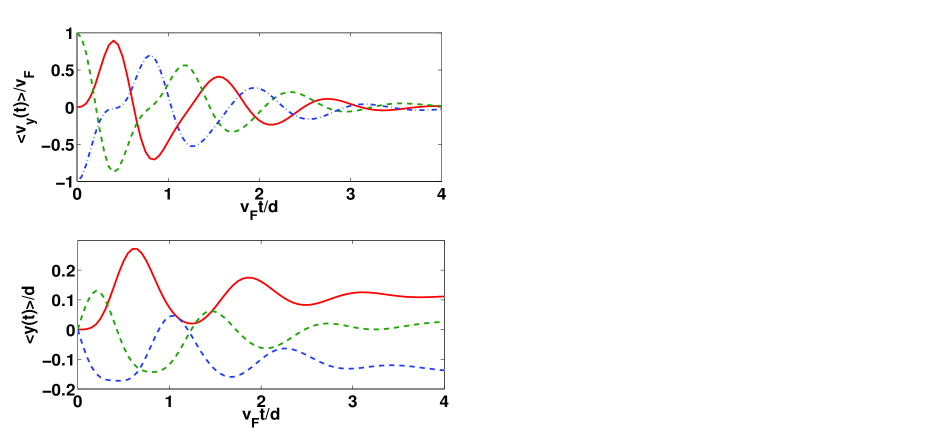
Figure 6: Time dependence of the expectation values of velocity and position operator when the initial pseudospin was polarized along $y$-direction. Here, solid(red), dashed(green), and dot-dashed(blue) lines correspond to different values of $(c_{1},c_{2},c_{3})$, namely, $(\sin\varphi,0,\cos\varphi)$, $(-i\cos\varphi,1,i\sin\varphi)$, and $(i\cos\varphi,1,-i\sin\varphi)$, respectively. We also consider $a=5$ and $\alpha=0.5$.

III In presence of a magnetic field

III.1 Energy spectrum

As a consequence of an external transverse magnetic field ${\bm{\mathcal{B}}}=\mathcal{B}\hat{z}$, the continuous energy spectrum of the conic band is redistributed in the form of following Landau levels :

$$\varepsilon_{n,\zeta}^{\lambda}=\lambda\,\gamma_{B}\sqrt{n+\chi_{\zeta}},$$ (28)

where $\lambda=\pm 1$ denotes either CB or VB, $n=0,1,2,...$ is the LL index, $\gamma_{B}=\sqrt{2}\hbar v_{F}/l_{0}$ with $l_{0}=\sqrt{\hbar/(e\mathcal{B})}$ being the magnetic length and $\chi_{\zeta}=[1-\zeta\cos(2\varphi)]/2$. It is important to note that the magnetic field can not alter the fate of the FB. It still retains its zero energy states.

Choosing the vector potential $\bm{\mathcal{A}}$ corresponding to ${\bm{\mathcal{B}}}$ in the Landau gauge as ${\bm{\mathcal{A}}}=(-\mathcal{B}y,0,0)$, we find the conic band eigenfunctions corresponding to the K-valley asdice_MagTr

$$\psi_{n,k_{x}}^{\lambda,{\rm K}}({\bf r})=\frac{1}{\sqrt{2}}\left(\begin{array}[]{c}\frac{\sqrt{n(1-\chi_{+})}}{\sqrt{n+\chi_{+}}}\Phi_{n-1}(y)\\ \lambda\Phi_{n}(y)\\ \frac{\sqrt{(n+1)\chi_{+}}}{\sqrt{n+\chi_{+}}}\Phi_{n+1}(y)\end{array}\right)\frac{e^{ik_{x}x}}{\sqrt{2\pi}}$$ (32)

and

$$\psi_{0,k_{x}}^{\lambda,{\rm K}}({\bf r})=\frac{1}{\sqrt{2}}\left(\begin{array}[]{c}0\\ \lambda\Phi_{0}(y)\\ \Phi_{1}(y)\end{array}\right)\frac{e^{ik_{x}x}}{\sqrt{2\pi}}$$ (36)

for $n>0$ and $n=0$, respectively. Here, $\Phi_{n}(y)=\sqrt{1/(2^{n}n!\sqrt{\pi}l_{0})}e^{-(y-y_{0})^{2}/(2l_{0}^{2})}H_{n}[(y-y_{0})/l_{0}]$, with $y_{0}=l_{0}^{2}k_{x}$, is the standard harmonic oscillator wave function.

On the other hand, despite its zero energy the FB wave functions for K-valley are obtained asdice_MagTr

$$\psi_{n,k_{x}}^{{\rm F},{\rm K}}({\bf r})=\left(\begin{array}[]{c}-\frac{\sqrt{(n+1)\chi_{+}}}{\sqrt{n+\chi_{+}}}\Phi_{n-1}(y)\\ 0\\ \frac{\sqrt{n(1-\chi_{+})}}{\sqrt{n+\chi_{+}}}\Phi_{n+1}(y)\end{array}\right)\frac{e^{ik_{x}x}}{\sqrt{2\pi}}$$ (40)

and

$$\psi_{0,k_{x}}^{{\rm F},{\rm K}}({\bf r})=\left(\begin{array}[]{c}0\\ 0\\ \Phi_{0}(y)\end{array}\right)\frac{e^{ik_{x}x}}{\sqrt{2\pi}},$$ (44)

for $n>0$ and $n=0$, respectively. Note that the states in the FB is infinitely degenerate.

III.2 Time evolution

Here we attempt to study the cyclotron dynamics of a quasiparticle represented by a wave packet. It should be mentioned here that we have considered the momentum-space wave packet in the case of zero magnetic field, but here we prefer to adopt position-space wave packet to circumvent calculation difficulties.

The initial Gaussian wave packet is chosen as

$$\Psi({\bf r},0)=\frac{1}{\sqrt{\pi}l_{0}C}\exp\Big{(}-\frac{r^{2}}{2l_{0}^{2}}+i\frac{p_{0x}x}{\hbar}\Big{)}\left(\begin{array}[]{c}c_{1}\\ c_{2}\\ c_{3}\end{array}\right),$$ (48)

where $p_{0x}$ is the initial momentum and the constants $c_{1}$, $c_{2}$, $c_{3}$ play the same role as mentioned in the case of zero external field.

To find the wave packet at a later time $t$, we need to construct suitable propagator that can describe the desired time evolution. In this way we follow the Green’s function technique given in Ref. [zb2d3, ] with appropriate modifications.

The time evolved wave packet can be found as

$$\Psi({\bf r},t)=\int d{\bf r^{\prime}}G({\bf r},{\bf r^{\prime}},t)\Psi({\bf r},0),$$ (49)

where the propagator or the Green’s function is given by

$$G({\bf r},{\bf r^{\prime}},t)=\begin{pmatrix}G_{11}&G_{12}&G_{13}\\ G_{21}&G_{22}&G_{23}\\ G_{31}&G_{32}&G_{33}\end{pmatrix}.$$ (50)

The matrix elements of $G({\bf r},{\bf r^{\prime}},t)$ are defined as

$$G_{lm}({\bf r},{\bf r^{\prime}},t)=\sum_{\lambda=\pm}\sum_{n=0}^{\infty}\psi_{n,k_{x},l}^{\lambda}({\bf r},t)\psi_{n,k_{x},m}^{\lambda^{\ast}}({\bf r},0),$$ (51)

where the time evolved state is given by $\psi_{n,k_{x},l}^{\lambda}({\bf r},t)=\psi_{n,k_{x},l}^{\lambda}({\bf r},0)e^{-i\varepsilon_{n}^{\lambda}t/\hbar}$.

The corresponding matrix elements i.e. $G_{lm}$’s can be found from the following equation

$$\begin{pmatrix}G_{11}\\ G_{21}\\ G_{31}\\ G_{12}\\ G_{22}\\ G_{32}\\ G_{13}\\ G_{23}\\ G_{33}\end{pmatrix}=\frac{1}{2\pi}\int dk_{x}e^{ik_{x}(x-x^{\prime})}\sum_{n=0}^{\infty}\begin{pmatrix}f_{n+1}(t)\phi_{n}(y-y_{c})\phi_{n}(y^{\prime}-y_{c})\\ g_{n+1}(t)\phi_{n+1}(y-y_{c})\phi_{n}(y^{\prime}-y_{c})\\ h_{n+1}(t)\phi_{n+2}(y-y_{c})\phi_{n}(y^{\prime}-y_{c})\\ g_{n+1}(t)\phi_{n}(y-y_{c})\phi_{n+1}(y^{\prime}-y_{c})\\ q_{n}(t)\phi_{n}(y-y_{c})\phi_{n}(y^{\prime}-y_{c})\\ p_{n}(t)\phi_{n+1}(y-y_{c})\phi_{n}(y^{\prime}-y_{c})\\ h_{n+1}(t)\phi_{n}(y-y_{c})\phi_{n+2}(y^{\prime}-y_{c})\\ p_{n}(t)\phi_{n}(y-y_{c})\phi_{n+1}(y^{\prime}-y_{c})\\ r_{n}(t)\phi_{n}(y-y_{c})\phi_{n}(y^{\prime}-y_{c})\end{pmatrix},$$ (52)

where $f_{n}(t)=A_{n}\cos(\delta_{n}t)+B_{n}$, $g_{n}(t)=-iC_{n}\sin(\delta_{n}t)$, $h_{n}(t)=D_{n}(\cos(\delta_{n}t)-1)$, $q_{n}(t)=\cos(\delta_{n}t)$, $p_{n}(t)=-iF_{n}\sin(\delta_{n}t)$, and $r_{n}(t)=B_{n-1}\cos(\delta_{n-1}t)+A_{n-1}$ with $A_{n}=n(1-\chi_{+})/(n+\chi_{+})$, $B_{n}=(n+1)\chi_{+}/(n+\chi_{+})$, $C_{n}=\sqrt{n(1-\chi_{+})/(n+\chi_{+})}$, $F_{n}=\sqrt{(n+1)\chi_{+}/(n+\chi_{+})}$, and $\delta_{n}=\gamma_{B}\sqrt{n+\chi_{+}}/\hbar$.

Now using Eq. (48), (49), and (52), we find the wave packet at a later time $t$ as

$$\left(\begin{array}[]{c}\Psi_{1}({\bf r},t)\\ \Psi_{2}({\bf r},t)\\ \Psi_{3}({\bf r},t)\end{array}\right)=\frac{1}{\sqrt{2}\pi l_{0}}\sum_{n=0}^{\infty}\frac{1}{2^{n}n!}\int due^{\Gamma(x,y,u)}(-u)^{n}\left(\begin{array}[]{c}\Sigma_{1}(t,u)\\ \Sigma_{2}(t,u)\\ \Sigma_{3}(t,u)\end{array}\right),$$ (59)

where $\Gamma(x,y,u)=iux/l_{0}-(p_{0x}l_{0}/\hbar-u)^{2}/2-u^{2}/4-(y/l_{0}-u)^{2}/2$ and $\Sigma_{\iota}(t,u)$’s with $\iota=1,2,3$ are given by the following matrix equation

$$\begin{pmatrix}\Sigma_{1}(t,u)\\ \Sigma_{2}(t,u)\\ \Sigma_{3}(t,u)\end{pmatrix}=\frac{1}{C}\begin{pmatrix}f_{n+1}(t)H_{n}(u)&-\frac{1}{\sqrt{2}}\frac{g_{n+1}(t)}{\sqrt{n+1}}uH_{n}(u)&\frac{1}{2}\frac{h_{n+1}(t)}{\sqrt{(n+1)(n+2)}}u^{2}H_{n}(u)\\ \frac{1}{\sqrt{2}}\frac{g_{n+1}(t)}{\sqrt{n+1}}H_{n+1}(u)&q_{n}(t)H_{n}(u)&-\frac{1}{\sqrt{2}}\frac{p_{n}(t)}{\sqrt{n+1}}uH_{n}(u)\\ \frac{1}{2}\frac{h_{n+1}(t)}{\sqrt{(n+1)(n+2)}}H_{n+2}(u)&\frac{1}{\sqrt{2}}\frac{p_{n}(t)}{\sqrt{n+1}}H_{n+1}(u)&r_{n}(t)H_{n}(u)\end{pmatrix}\begin{pmatrix}c_{1}\\ c_{2}\\ c_{3}\end{pmatrix}.$$ (60)

III.3 Expectation values

The expectation value of the velocity operator can be written in the following form as

$$\begin{pmatrix}\langle v_{x}(t)\rangle\\ \langle v_{y}(t)\rangle\end{pmatrix}=2v_{F}\begin{pmatrix}{\rm Re}\\ {\rm Im}\end{pmatrix}\Big{[}\cos\varphi I_{12}(t)+\sin\varphi I_{23}(t)\Big{]},$$ (61)

where, $I_{\mu\sigma}(t)$ is defined as $I_{\mu\sigma}(t)=\int\Psi_{\mu}^{\ast}({\bf r},t)\Psi_{\sigma}({\bf r},t)dxdy$. After a straightforward calculation we evaluate $I_{12}(t)$ and $I_{23}(t)$ as

$$I_{12}(t) = \sqrt{\frac{2}{3}}\frac{1}{C^{2}}\sum_{n=0}^{\infty}\frac{1}{2^{n}n!}\Bigg{[}c_{1}^{\ast}c_{2}f_{n+1}^{\ast}q_{n}\xi_{2n}+\frac{1}{\sqrt{2(n+1)}}\Big{\{}|c_{1}|^{2}f_{n+2}^{\ast}g_{n+1}+c_{1}^{\ast}c_{3}f_{n+1}^{\ast}p_{n}+|c_{2}|^{2}g_{n+1}^{\ast}q_{n}\Big{\}}\xi_{2n+1}$$ (62)

$$+ \frac{1}{2\sqrt{(n+1)(n+2)}}\Big{\{}c_{3}^{\ast}c_{2}h_{n+1}^{\ast}q_{n}+c_{2}^{\ast}c_{1}g_{n+2}^{\ast}g_{n+1}+c_{2}^{\ast}c_{3}\sqrt{\frac{n+2}{n+1}}g_{n+1}^{\ast}p_{n}\Big{\}}\xi_{2n+2}$$

$$+ \frac{1}{2\sqrt{2(n+1)(n+2)(n+3)}}\Big{\{}c_{3}^{\ast}c_{1}h_{n+2}^{\ast}g_{n+1}+|c_{3}|^{2}\sqrt{\frac{n+3}{n+1}}h_{n+1}^{\ast}p_{n}\Big{\}}\xi_{2n+3}\Bigg{]}$$

and

$$I_{23}(t) = \sqrt{\frac{2}{3}}\frac{1}{C^{2}}\sum_{n=0}^{\infty}\frac{1}{2^{n}n!}\Bigg{[}\Big{\{}c_{1}^{\ast}c_{2}g_{n+1}^{\ast}p_{n}+c_{2}^{\ast}c_{3}q_{n}^{\ast}r_{n}\Big{\}}\xi_{2n}+\frac{1}{\sqrt{2(n+1)}}\Big{\{}|c_{1}|^{2}g_{n+2}^{\ast}h_{n+1}+c_{1}^{\ast}c_{3}g_{n+1}^{\ast}r_{n+1}$$ (63)

$$+ |c_{2}|^{2}q_{n+1}^{\ast}p_{n}+|c_{3}|^{2}p_{n}^{\ast}r_{n}\Big{\}}\xi_{2n+1}+\frac{1}{2\sqrt{(n+1)(n+2)}}\Big{\{}c_{2}^{\ast}c_{1}q_{n+2}^{\ast}h_{n+1}+c_{3}^{\ast}c_{2}p_{n+1}^{\ast}p_{n}\Big{\}}\xi_{2n+2}$$

$$+ \frac{1}{2\sqrt{2(n+1)(n+2)(n+3)}}c_{3}^{\ast}c_{1}\frac{p_{n+2}^{\ast}h_{n+1}}{\sqrt{(n+1)(n+2)(n+3)}}\xi_{2n+3}\Bigg{]},$$

where

$$\xi_{m}=(-1)^{m}\Big{(}\frac{2}{3}\Big{)}^{\frac{m}{2}}{\rm exp}\bigg{(}-\frac{p_{0x}^{2}l_{0}^{2}}{3\hbar^{2}}\bigg{)}\frac{H_{m}(i\sqrt{\frac{2}{3}}\frac{p_{0x}l_{0}}{\hbar})}{(2i)^{m}}.$$ (64)

III.4 Different choices of initial pseudospin polarization

Likewise the zero magnetic field case we discuss here the behavior of ZB for various choices of initial pseudospin polarization corresponding to the different values of $c_{1}$, $c_{2}$, and $c_{3}$.

1.  z-polarization

We consider the pseudospin associated with the initial wave packet is polarized along the $z$-direction. Similar to the zero field case, here we also have three distinct choices of $(c_{1},c_{2},c_{3})$, namely, $(1,0,0)$, $(0,1,0)$, and $(0,0,1)$. In the following we demonstrate how different choices of $(c_{1},c_{2},c_{3})$ lead to modify the structure of ZB.

(i) For $(c_{1},c_{2},c_{3})=(1,0,0)$ we find from Eq. (62) and Eq. (63)

$$I_{12}(t)=\frac{1}{\sqrt{3}}\sum_{n=0}^{\infty}\frac{f_{n+2}^{\ast}g_{n+1}}{2^{n}n!\sqrt{n+1}}\xi_{2n+1}.$$ (65)

$$I_{23}(t)=\frac{1}{\sqrt{3}}\sum_{n=0}^{\infty}\frac{g_{n+2}^{\ast}h_{n+1}}{2^{n}n!\sqrt{n+1}}\xi_{2n+1}.$$ (66)

Note that the products $f_{n+2}^{\ast}g_{n+1}$ and $g_{n+2}^{\ast}h_{n+1}$ are purely imaginary. As a result, we readily obtain from Eq. (61) that $\langle v_{x}(t)\rangle=0$ and

$$\langle v_{y}(t)\rangle = \frac{2v_{F}}{\sqrt{3}}\sum_{n=0}^{\infty}\frac{\xi_{2n+1}}{2^{n}n!\sqrt{n+1}}{\rm Im}\Big{(}\cos\varphi\,f_{n+2}^{\ast}g_{n+1}$$ (67)

$$+ \sin\varphi\,g_{n+2}^{\ast}h_{n+1}\Big{)}.$$

(ii) For $(c_{1},c_{2},c_{3})=(0,1,0)$ we find $\langle v_{x}(t)\rangle=0$ and

$$\langle v_{y}(t)\rangle = \frac{2v_{F}}{\sqrt{3}}\sum_{n=0}^{\infty}\frac{\xi_{2n+1}}{2^{n}n!\sqrt{n+1}}{\rm Im}\Big{(}\cos\varphi\,g_{n+1}^{\ast}q_{n}$$ (68)

$$+ \sin\varphi\,q_{n+1}^{\ast}p_{n}\Big{)}.$$

(iii) When $(c_{1},c_{2},c_{3})=(0,0,1)$, it is obtained that $\langle v_{x}(t)\rangle=0$ and

$$\langle v_{y}(t)\rangle = \frac{2v_{F}}{\sqrt{3}}\sum_{n=0}^{\infty}\frac{1}{2^{n}n!\sqrt{n+1}}{\rm Im}\Big{(}\sin\varphi\,p_{n}^{\ast}r_{n}\xi_{2n+1}$$ (69)

$$+ \frac{\cos\varphi}{2\sqrt{(n+1)(n+2)}}h_{n+1}^{\ast}p_{n}\xi_{2n+3}\Big{)}.$$

A careful inspection of Eq. (67)-(69) reveals that the structure of the ZB appeared in velocity significantly depends on different choices of $(c_{1},c_{2},c_{3})$.

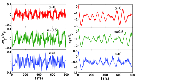
Figure 7: Expectation values of position and velocity operators in presence of a transverse magnetic field for pseudo spin polarization along $z$-direction with components $(c_{1},c_{2},c_{3})$=$(1,0,0)$. Here, we consider $k_{0x}=2\times 10^{8}$ m^-1 and $l_{0}$=$8.11$ nm.

In all cases the velocity average undergoes multi-frequency transverse ZB governed by the interference among different Landau levels. In Fig. 7 - Fig. 9 we portray the time dependence of the expectation values of velocity and position operators. With appropriate initial conditions taken into account corresponding position expectation values can be obtained by integrating Eqs. (67)-(69). The actual initial condition is $\langle y\rangle=\langle y_{0}\rangle=k_{0x}l_{0}^{2}$ at $t=0$. To calculate $\langle y(t)\rangle$ we choose the following initial condition : $\langle y\rangle=0$ at $t=0$. The expectation values of position operator as illustrated in Fig. 7 - Fig. 9 differ from their actual values at most by a constant shift $\langle y_{0}\rangle$. We perform all the calculations for a constant magnetic field $\mathcal{B}=10$ T for which the magnetic length scale becomes $l_{0}=8.11$ nm. We also consider the width of the wave packet as $d=l_{0}$. Fig. 7 illustrates the ZB appeared in velocity and position for various values of $\alpha$. In this case we choose $(c_{1},c_{2},c_{3})=(1,0,0)$ and $k_{0x}=2\times 10^{8}$ m^-1. It is clear from Fig. 7, the ZBs appeared in both position and velocity undergo perform permanent oscillations and oscillatory patterns depend significantly on $\alpha$.

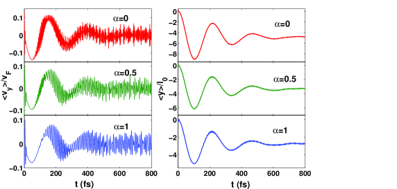
Figure 8: Expectation values of position and velocity operators in presence of a transverse magnetic field for pseudo spin polarization along $z$-direction with components $(c_{1},c_{2},c_{3})=(1,0,0)$. Here, we consider $k_{0x}$=$6\times 10^{8}$ m^-1 and $l_{0}$=$8.11$ nm.

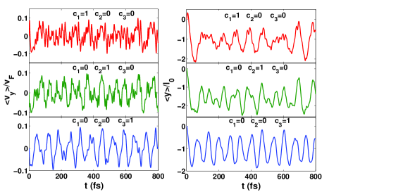
Figure 9: Expectation values of position and velocity operators in presence of a transverse magnetic field for pseudospin polarization along $z$-direction with different combinations of $(c_{1},c_{2},c_{3})$. Here, we consider $k_{0x}$=$2\times 10^{8}$ m^-1, $l_{0}$=$8.11$ nm, and $\alpha$=$0.5$.

To plot Fig. 8 we repeat the calculations for a higher value of $k_{0x}$, namely, $k_{0x}=6\times 10^{8}$ m^-1. In this case the ZB in position exhibits transient character. However, for ZB in velocity a highly oscillatory pattern is superimposed on the transient character. Note that the locations of maxima and minima are almost insensitive to $\alpha$. Only the amplitude of ZB changes with $\alpha$.

Fig. 9 describe the behavior of ZB corresponding to different possibilities of $(c_{1},c_{2},c_{3})$. For the plots, we have taken $k_{0x}=2\times 10^{8}$ m^-1 and $\alpha=0.5$. Here, the oscillatory pattern is significantly different for different initial pseudospin polarization.

2.  x-polarization

Here, we consider that the initial wave packet was polarized along $x$-direction and the resultant behaviors are shown in Fig. 10 and Fig. 11. As mentioned earlier we have following choices of $(c_{1},c_{2},c_{3})$, namely, $(\sin\varphi,0,-\cos\varphi)$, $(\cos\varphi,1,\sin\varphi)$, and $(-\cos\varphi,1,-\sin\varphi)$. In this case the values of parameters are taken as $k_{0x}$=$2\times 10^{8}$ m^-1, $\alpha$=$0.5$, and $l_{0}$=$8.11$ nm.

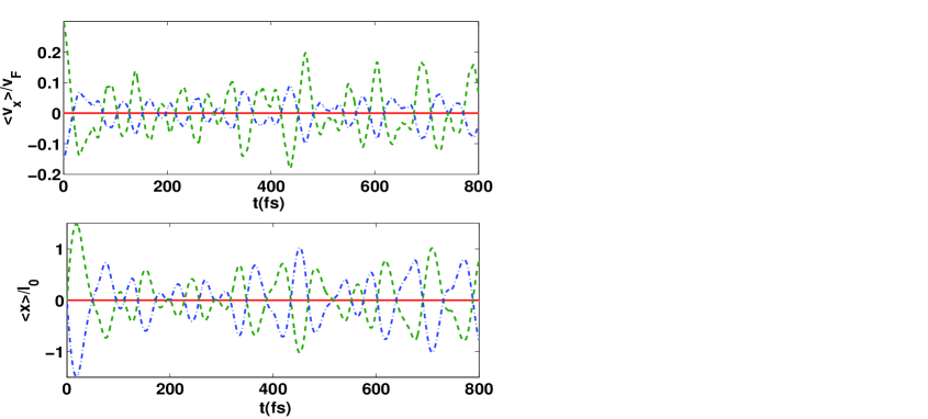
Figure 10: Time dependence of the expectation values of $x$-component of velocity and position operators when the initial pseudospin was polarized along $x$-direction. Here, solid(red), dashed(green), and dot-dashed(blue) lines correspond to different values of $(c_{1},c_{2},c_{3})$, namely, $(\sin\varphi,0,-\cos\varphi)$, $(\cos\varphi,1,\sin\varphi)$, and $(-\cos\varphi,1,-\sin\varphi)$, respectively. We also consider $k_{0x}$=$2\times 10^{8}$ m^-1, $l_{0}$=$8.11$ nm, and $\alpha$=$0.5$.

Interestingly we find that the $x$-component of the expectation values of velocity and position operators are non-zero as evident from Fig. 10. However, for $(c_{1},c_{2},c_{3})=(\sin\varphi,0,-\cos\varphi)$, it is obtained that $\langle v_{x}(t)\rangle=0$ and $\langle x(t)\rangle=0$. The expectation values of $x$ corresponding to other choices of $(c_{1},c_{2},c_{3})$ are mirror images of each other. This particular feature was also reflected in the case of zero magnetic field. However, the values of $\langle v_{x}(t)\rangle$ corresponding to $(c_{1},c_{2},c_{3})=(\cos\varphi,1,\sin\varphi)$ and $(c_{1},c_{2},c_{3})=(-\cos\varphi,1,-\sin\varphi)$ are not exactly mirror images of each other. In fact, the amplitude of $\langle v_{x}(t)\rangle$ in the first case is greater than that in the second case.

On the other hand, the time dependence of the expectation values of $y$ and $v_{y}$ are portrayed in Fig. 11. Both $\langle y(t)\rangle$ and $\langle v_{y}(t)\rangle$ exhibit regular oscillations for $(c_{1},c_{2},c_{3})=(\sin\varphi,0,-\cos\varphi)$. Irregularities in the oscillations appear for other choices of $(c_{1},c_{2},c_{3})$.

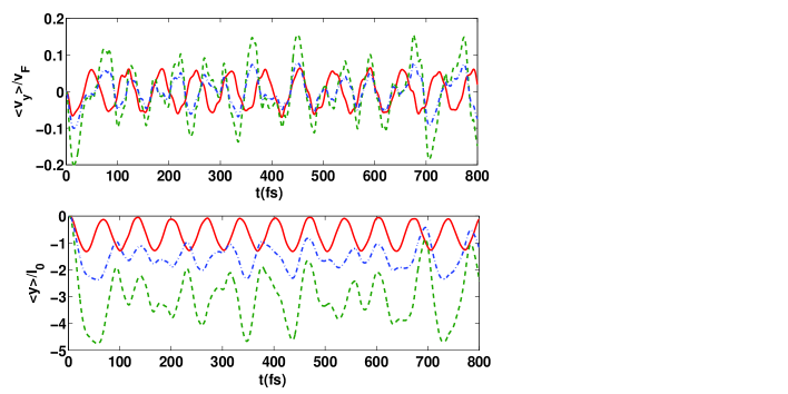
Figure 11: Time dependence of the expectation values of $y$-component of velocity and position operators when the initial pseudospin was polarized along $x$-direction. Here, solid(red), dashed(green), and dot-dashed(blue) lines correspond to different values of $(c_{1},c_{2},c_{3})$, namely, $(\sin\varphi,0,-\cos\varphi)$, $(\cos\varphi,1,\sin\varphi)$, and $(-\cos\varphi,1,-\sin\varphi)$, respectively. We also consider $k_{0x}$=$2\times 10^{8}$ m^-1, $l_{0}$=$8.11$ nm, and $\alpha$=$0.5$.

3.  y-polarization

Finally, we depict the time dependence of the expectation values of position and velocity operators in Fig. 12 by considering the initial pseudospin polarization was along $y$-direction. We have the following choices of $(c_{1},c_{2},c_{3})$ such as $(\sin\varphi,0,\cos\varphi)$, $(-i\cos\varphi,1,i\sin\varphi)$, and $(i\cos\varphi,1,-i\sin\varphi)$. We take same parameter values as considered for choice 2. Similar to choice 1, we obtain $\langle x(t)\rangle=0$ and $\langle v_{x}(t)\rangle=0$. For all possibilities of $(c_{1},c_{2},c_{3})$, complicated irregular oscillatory patterns are obtained in both $\langle y(t)\rangle$ and $\langle v_{y}(t)\rangle$.

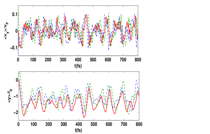
Figure 12: Time dependence of the expectation values of $y$-component of velocity and position operators when the initial pseudospin was polarized along $y$-direction. Here, solid(red), dashed(green), and dot-dashed(blue) lines correspond to different values of $(c_{1},c_{2},c_{3})$, namely, $(\sin\varphi,0,\cos\varphi)$, $(-i\cos\varphi,1,i\sin\varphi)$, and $(i\cos\varphi,1,-i\sin\varphi)$, respectively. We also consider $k_{0x}$=$2\times 10^{8}$ m^-1, $l_{0}$=$8.11$ nm, and $\alpha$=$0.5$.

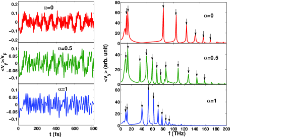
Figure 13: The Left panel shows the time dependence of $\langle v_{y}(t)\rangle$ for $z$-polarized wave packet with components $c_{1}$=$1$, $c_{2}$=$0$, and $c_{3}$=$0$. The right panel displays corresponding Fourier transforms of $\langle v_{y}(t)\rangle$. The downward arrows depict the frequency values. We consider $k_{0x}$=$2\times 10^{8}$ m^-1 and $l_{0}$=$8.11$ nm.

Freq. (THz)	$\alpha$=$0$	$\alpha$=0.5	$\alpha$=1
$f_{1}$	$10.99$	$9.76$	$9.76$
$f_{2}$	$13.43$	$13.43$	$12.21$
$f_{3}$	$80.59$	$36.63$	$40.29$
$f_{4}$	$105.00$	$48.84$	$52.50$
$f_{5}$	$124.50$	$59.83$	$62.27$
$f_{6}$	$141.60$	$68.38$	$70.82$
$f_{7}$	$156.30$	$75.70$	$78.14$
$f_{8}$	$169.70$	$85.47$	$85.47$
$f_{9}$	$-$	$108.70$	$91.58$
$f_{10}$	$-$	$128.20$	$-$
$f_{11}$	$-$	$144.10$	$-$
$f_{12}$	$-$	$158.70$	$-$

Table 1: Frequency involved in ZB for different values of $\alpha$ obtained from Fig. 13.

III.5 Determination of frequencies involved in ZB

It would be interesting to find out the frequency components which are present in the complicated structure of ZB. As an example we consider the case in which the wave packet was polarized initially along $z$-direction with components $c_{1}$=$1$, $c_{2}$=$0$, and $c_{3}$=$0$. The time dependence of $\langle v_{y}(t)\rangle$ and $\langle y(t)\rangle$ are already shown in Fig. 7. We make fast Fourier transformation of $\langle v_{y}\rangle$ vs $t$ data to find the frequencies involved in ZB. The corresponding results are shown in Fig. 13. The arrows in the right panels of Fig. 13 denote the frequencies involved in ZB. The revealed frequencies corresponding to different values of $\alpha$ are given in Table I. Note that the number of frequency components depends on $\alpha$ significantly. We find, approximately, $8$, $12$, and $9$ frequencies for $\alpha$=$0$, $\alpha$=$0.5$, and $\alpha$=$1$, respectively. These frequencies are governed by all possible differences between Landau energy levels. In a similar way one can also find out the frequencies corresponding to the other choices of $c_{1}$, $c_{2}$, and $c_{3}$.

IV Summary

In summary, we have studied ZB of a Gaussian wave packet which represents a quasiparticle in $\alpha$-T₃ model. We also consider the effect of an external transverse magnetic field on ZB. The manifestation of ZB of wave packet is shown in the expectation values of physical observables like position and velocity. For zero magnetic field case, we find that the ZBs appeared in position and velocity diminish with time. The problem studied in this article is an example of two frequency ZB for a finite values of $\alpha$ e.g. $0<\alpha<1$. One frequency is originating due to the interference between conduction and valence band whereas the other frequency is a result of interference between either conduction and flat band or flat and valence band. It is revealed that ZB depends significantly on the nature of the initial pseudospin polarization. Specifically, the case with initial pseudospin polarization along $z$-direction is more interesting. By considering this particular spin polarization we find that ZB consists of two aforesaid frequencies for $0<\alpha<1$ when the initial wave packet was completely located in any of the $rim$ sites. A transition from $2\Omega_{q}$-frequency ZB to $\Omega_{q}$-frequency ZB is unveiled as $\alpha$ is varied from $0$ to $1$. On contrary, the existence of a single $2\Omega_{q}$-frequency ZB is realized for a finite $\alpha$ in the case of initial wave packet being situated in the $hub$ site. The timescales over which the ZB persists can be extracted from the approximate results of expectation values obtained in the large width limit of the wave packet. Other choices of initial pseudospin polarization have produced some interesting features. In presence of a finite magnetic field the ZB displays complicated permanent oscillations as a result of interference among large number of Landau levels. Similar to zero magnetic field case the oscillatory pattern depends on the type of initial pseudospin polarization.

References

- (1) E. Schrödinger, Sitzungsber. Preuss. Akad. Wiss., Phys. Math. Kl. 24, 418 (1930); A. O. Barut and A. J. Bracken, Phys. Rev. D 23, 2454 (1981).
- (2) W. Zawadzki, Phys. Rev. B 72, 085217 (2005).
- (3) W. Zawadzki and T. M. Rusin, J. Phys.: Condens. Matter 23, 143201 (2011).
- (4) J. Schliemann, D. Loss, and R. M. Westervelt, Phys. Rev. Lett. 94, 206801 (2005).
- (5) S. Q. Shen, Phys. Rev. Lett. 95, 187203 (2005).
- (6) J. Schliemann, D. Loss, and R. M. Westervelt, Phys. Rev. B 73, 085323 (2006).
- (7) V. Ya. Demikhovskii, G. M. Maksimova, and E. V. Frolova, Phys. Rev. B 78, 115401 (2008).
- (8) T. Biswas and T. K. Ghosh, J. Phys.: Condens. Matter 24, 185304 (2012).
- (9) C. S. Ho, M. B. A. Jalil, and S. G. Tan, EPL, 108, 27012 (2014).
- (10) T. Biswas and T. K. Ghosh, J. Appl. Phys. 115, 213701 (2014).
- (11) T. Biswas, S. Chowdhury, and T. K. Ghosh, Eur. Phys. J. B 88, 220 (2015).
- (12) J. Cserti and G. David, Phys. Rev. B 74, 172305 (2006).
- (13) X. Zhang and Z. Liu, Phys. Rev. Lett. 101, 264303 (2008).
- (14) X. Zhang, Phys. Rev. Lett. 100, 113903 (2008).
- (15) F. Dreisow, M. Heinrich, R. Keil, A. Tunnermann, S. Nolte, S. Longhi, and A. Szameit, Phys. Rev. Lett. 105, 143902 (2010).
- (16) W. Zawadzki, Phys. Rev. B 74, 205439 (2006).
- (17) T. M. Rusin and W. Zawadzki, Phys. Rev. B 76, 195439 (2007).
- (18) T. M. Rusin and W. Zawadzki, Phys. Rev. B 78, 125419 (2008).
- (19) G. M. Maksimova, V. Ya. Demikhovskii, and E. V. Frolova, Phys. Rev. B 78, 235321 (2008).
- (20) J. Schliemann, New J. Phys. 10, 043024 (2008).
- (21) Q. Wang, R. Shen, L. Sheng, B. G. Wang, and D. Y. Xing, Phys. Rev. A 89, 022121 (2014).
- (22) L. K. Shi, S. C. Zhang, and K. Chang, Phys. Rev. B 87, 161115 (R) (2013).
- (23) A. Singh, T. Biswas, T. K. Ghosh, and A. Agarwal, Eur. Phys. J. B 87, 275 (2014).
- (24) A. Singh, T. Biswas, T. K. Ghosh, and A. Agarwal, Ann. Phys. 354, 274 (2015).
- (25) J. Y. Vaishnav and C. W. Clark, Phys. Rev. Lett. 100, 153002 (2008).
- (26) Y. C. Zhang, S. W. Song, C. F. Liu, and W. M. Liu, Phys. Rev. A 87, 023612 (2013).
- (27) L. J. LeBlanc, M. C. Beeler, K. Jimenez-Garcia, A. R. Perry, S. Sugawa, R. A. Williams, and I. B. Spielman, New J. Phys. 15, 073011 (2013).
- (28) C. Qu, C. Hamner, M. Gong, C. Zhang, and P. Engels, Phys. Rev. A 88, 021604(R) (2013).
- (29) K. Huang, Am. J. Phys. 20, 479 (1952).
- (30) J. Cserti and G. David, Phys. Rev. B 82, 201405 (2010).
- (31) J. A. Lock, Am. J. Phys. 47, 797 (1979).
- (32) M. I. Katsnelson, Eur. Phys. J. B 51, 157 (2006).
- (33) Y. Iwasaki, Y. Hashimoto, T. Nakamura, and S. Katsumoto, Sci. Rep. 7, 7909 (2017).
- (34) B. Dora, J. Kailasvuori, and R. Moessner, Phys. Rev. B 84, 195422 (2011).
- (35) Z. Lan, N. Goldman, A. Bermudez, W. Lu, and P. Öhberg, Phys. Rev. B 84, 165115 (2011).
- (36) J. D. Malcolm and E. J. Nicol, Phys. Rev. B 90, 035405 (2014).
- (37) B. Sutherland, Phys. Rev. B 34, 5208 (1986).
- (38) J. Vidal, R. Mosseri, and B. Doucot, Phys. Rev. Lett. 81, 5888 (1998).
- (39) S. E. Korshunov, Phys. Rev. B 63, 134503 (2001͒).
- (40) M. Rizzi, V. Cataudella, and R. Fazio, Phys. Rev. B 73, 144511 (2006͒).
- (41) D. F. Urban, D. Bercioux, M. Wimmer, and W. Häusler, Phys. Rev. B 84, 115136 (2011).
- (42) T. Louvet, P. Delplace, A. A. Fedorenko, and D. Carpentier, Phys. Rev. B 92, 155116 (2015).
- (43) J. D. Malcolm and E. J. Nicol, Phys. Rev. B 93, 165433 (2016).
- (44) D. Bercioux, D. F. Urban, H. Grabert, and W. Häusler, Phys. Rev. A 80, 063603 (2009).
- (45) F. Wang and Y. Ran, Phys. Rev. B 84, 241103 (2011).
- (46) A. Raoux, M. Morigi, J.-N. Fuchs, F. Piechon, and G. Montambaux, Phys. Rev. Lett. 112, 026402 (2014).
- (47) J. D. Malcolm and E. J. Nicol, Phys. Rev. B 92, 035118 (2015).
- (48) T. Biswas and T. K. Ghosh, J. Phys.: Condens. Matter 28, 495302 (2016).
- (49) E. Illes, J. P. Carbotte, and E. J. Nicol, Phys. Rev. B 92, 245410 (2015).
- (50) E. Illes, and E. J. Nicol, Phys. Rev. B 94, 125435 (2016).
- (51) A. D. Kovacs, G. David, B. Dora, and J. Cserti, Phys. Rev. B 95, 035414 (2017).
- (52) E. Illes, and E. J. Nicol, Phys. Rev. B 95, 235432 (2017).
- (53) SK F. Islam and P. Dutta, Phys. Rev. B 96, 045418 (2017).