Linear guided modes and Whitham-Boussinesq model for variable topography

Abstract

In this article we study two classical linear water wave problems, i) normal modes of infinite straight channels of bounded constant cross-section, and ii) trapped longitudinal modes in domains with unbounded constant cross-section. Both problems can be stated using linearized free surface potential flow theory, and our goal is to compare known analytic solutions in the literature to numerical solutions obtained using an ad-hoc but simple approximation of the non-local Dirichlet-Neumann operator for linear waves proposed in [1]. To study normal modes in channels with bounded cross-section we consider special symmetric triangular cross-sections, namely symmetric triangles with sides inclined at $45^{\circ}$ and $60^{\circ}$ to the vertical, and compare modes obtained using the non-local Dirichlet-Neumann operator to known semi-exact analytic expressions by Lamb [2], Macdonald [3] , Greenhill [4], Packham [5], and Groves [6]. These geometries have slopping beach boundaries that should in principle limit the applicability of our approximate Dirichlet-Neumann operator. We nevertheless see that the operator gives remarkably close results for even modes, while for odd modes we have some discrepancies near the boundary. For trapped longitudinal modes in domains with an infinite cross-section we consider a piecewise constant depth profile and compare modes computed with the nonlocal operator modes to known analytic solutions of linearized shallow water theory by Miles [7], Lin, Juang and Tsay [8], see also [9]. This is a problem of significant geophysical interest, and the proposed model is shows to give quantitatively similar results for the lowest trapped modes.

Keywords: linear water waves, variable topography, exact results, nonlocal shallow water wave models, transverse modes, continental shelves, triangular channels

1 Introduction

We study some problems on normal modes in linear water wave theory, in particular we compute numerically i) transverse normal modes in an infinite straight channel of bounded cross-section, and ii) trapped modes in domains with an unbounded cross-section. In both cases we consider special depth profiles for which we have known explicit or semi-explicit analytical solutions. The main goal of this paper is to compare these solutions to numerical solutions obtained using a simple approximate nonlocal version of the water wave equations for variable depth that was recently proposed for dispersive shallow water waves [1]. In the case of transverse modes we compare modes of the approximate model of [1] to the known semi-analytic solutions for a channel with triangular cross-section [6, 5, 2, 3, 4]. In the study of trapped modes we compare the predictions of the model of [1] to results obtained by the commonly used non-dispersive shallow water theory, applied to a model continental shelf geometry considered by several authors [10, 11, 8, 9, 7].

The nonlocal linear system we use to compute normal modes is derived using the Hamiltonian formulation of the free surface potential flow [12], see also [13], [14] and by approximating the (nonlocal) Dirichlet-Neumann operator for the Laplacian in the fluid domain appearing in the kinetic energy part of the Hamiltonian [15]. Explicit expressions for the Dirichlet-Neumann operator in variable depth were derived by Craig, Guyenne, Nicholls and Sulem [16], see also [17]. Such expressions are generally complicated and can be used for numerical computations [18], or to further simplify the equations of motion. [1] proposed an ad-hoc simplification of the variable depth Dirichlet-Neumann operator that leads to a simple variable depth generalization of Whitham-Boussinesq equations for shallow water theory. Nonlocal unidirectional and bidirectional shallow water models are of considerable current interest as nonlocal extensions of well-studied dispersive shallow water wave models such as the KdV and Boussinesq equations [19, 20]. We mention results on the existence of periodic traveling waves [21], solitary waves [22], wave breaking [23, 24, 25] and limiting Stokes waves [26]. The inclusion of variable depth effects is clearly of interest in geophysical and coastal engineering applications, and raises additional questions on the dynamics of these systems.

An immediate consequence of the Hamiltonian and Dirichlet-Neumann formulation of the water wave problem is that variable depth effects are already captured at the level of the linear theory. For instance, the Dirichlet-Neumann operator can be expressed recursively in terms of the zero wave-amplitude Dirichlet-Neuman operator [16]. The study of linear normal modes is therefore a good test problem for comparing different approximations of the Dirichlet-Neumann operator for variable depth.

The first part of the present work examines normal modes obtained by the approximate Dirichlet-Neumann operator for special depth profiles that admit known semi-analytic normal mode solutions of the linearized water wave problem. These analytical results concern a few special depth profiles such as isosceles triangles with sides inclined at $45^{\circ}$ and $60^{\circ}$ to the vertical, see Greenhill [4], Macdonald [3], and the summary in Lamb’s book, [2]. More recent studies are by Packham [5] and Groves [6]. A complete set of modes was also obtained for a semicircular channel by Evans and Linton [27]. The construction yields odd and even normal modes that we then compare to odd and even eigenfunctions of suitable approximate Dirichlet-Neumann operator in a periodic domain (the period is the base of the triangle). As we clarify in the next sections, the two problems are not equivalent because of the different assumptions at the intersection between the horizontal and sloping beach boundaries. (All known non-constant depth examples with analytic solutions concern domains with a sloping beach.) Despite this problem, examining these examples we see that the two approaches give comparable and often very close results for the normal mode shape, especially away from the beach. This is especially the case for higher even modes, where we see good agreement in the entire domain. Results for odd modes are close away from the beach, but have a marked discrepancy near the beach. We also see that approximating the triangular domain by a domain with a vertical wall (or a suitable periodic analogue) yields modes that approach the triangular domain modes as the height of the wall vanishes.

The second problem we study are trapped longitudinal modes in 3-D channels with a constant unbounded cross-section. The depth of the cross section is piecewise constant and takes two values, with the smaller depth defined over a finite interval. Longitudinal modes are assumed to have a sinusoidal dependence in the longitudinal direction, and trapped longitudinal modes are solutions that decay at infinity in the transverse horizontal direction. The two-level step depth profile has been used by many authors Miles [7], Lin et al. [8], Mei et al. [9], to model localized waves that travel along continental shelves. These studies use a St. Venant-type linear shallow wave theory that leads to exact solutions and an algebraic determination of the number of trapped solutions with a given longitudinal speed. Trapped modes obtained using this approach are compared to numerical eigenfunctions of a higher dimensional analogue of the model Dirichlet-Neumann operator of [1]. We see a good qualitative agreement to the trapped modes computed exactly, but it remains an open problem whether the two operators predict the same number of trapped states.

The organization of the paper is as follows. In Section 2 we formulate the linear water wave problem and present the nonlocal operators used to approximate the linear system. In Section 3 we consider triangular depth geometries, review some of the known semi-analytic normal mode solutions, and compare them to to numerical eigenmodes computed using the approximate nonlocal operator. In Section 4 we compute the semi-exact longitudinal mode solutions of the shallow water theory in a simple geometry used in the literature to model two continental shelves, and compare with results obtained using the nonlocal model.

2 Formulation of the problem and approximate
Dirichlet-Neumann operators

The problems considered in this paper come from the classical linear theory of water waves [2]. To describe the equations we use Cartesian coordinates denoted by $(x,y,z)$, where $y$ is directed vertically upwards, $x$ is measured longitudinally along the channel and $z$ is measured across the channel or across the submarine ridge, see e.g. Figures 1(a), 1(b), 2.

We define the fluid domain as $\mathcal{D}=\mathbb{R}\times\Omega,$ where $\Omega$ is the cross section, and we distinguish bounded and unbounded cross sections $\Omega=\Omega_{B}$, $\Omega_{U}$ respectively, with

$$\Omega_{B}=\{[z,y]:z\in[0,b],y\in[h_{m}+\beta(z),h_{M}],$$ (2.1)

$$\Omega_{U}=\{[z,y]:z\in\mathbb{R},y\in[h_{m}+\beta(z),h_{M}].$$ (2.2)

The heights $y=h_{m}$ and $y=h_{M}$ describe the minimum and maximum elevations respectively, with $h_{m}<h_{M}$, and $h_{m}+\beta(z)\leq h_{M}$ for all $z$.

We will assume $\partial\mathcal{D}=\mathbb{R}\times\partial\Omega=\Gamma_{L}\cup\Gamma_{F}\cup\Gamma_{B}$, with $\Gamma_{L}$ representing the lateral wall, $\Gamma_{F}$ representing the free surface and $\Gamma_{B}$ the bottom.

In the case $\Omega=\Omega_{B}$ we have

$$\Gamma_{F}=\{(x,h_{M},z):x\in\mathbb{R},0\leq z\leq b\},$$ (2.3)

$$\Gamma_{B}=\{(x,h_{m}+\beta(z),z):x\in\mathbb{R},0\leq z\leq b\},$$ (2.4)

$$\Gamma_{L}=\{(x,y,0):x\in\mathbb{R},y\in[h_{m}+\beta(0),h_{M}]\}\cup\{(x,y,b):x\in\mathbb{R},y\in[h_{m}+\beta(b),h_{M}]\}.$$ (2.5)

In this article are primarily interested in domains with $h_{m}+b(z)=h_{M}$ at $z=0$ and $b$. Then $\Gamma_{L}=\emptyset$.

In the case $\Omega=\Omega_{U}$ we are interested in domains with $\beta(z)\rightarrow 0$ as $z\rightarrow\pm\infty$.

To state the problem we introduce a velocity potential $\phi(x,y,z,t)$ and look for solutions of Laplace’s equation

$$\phi_{xx}+\phi_{yy}+\phi_{zz}=0\text{ in }\mathcal{D,}$$ (2.6)

with

$$\left\{\begin{array}[]{l}\phi_{t}+g\eta=0\text{ on }\Gamma_{F},\\ \eta_{t}=\varphi_{y}\text{ on }\Gamma_{F},\\ \frac{\partial\phi}{\partial{\hat{n}}}=0\text{ on }\Gamma_{B}\cup\Gamma_{L},\end{array}\right.$$ (2.7)

see [28]. Equations (2.6), (2.7) are the linearized Euler equations for free surface potential flow.

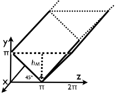
(a) $\beta_{45}$

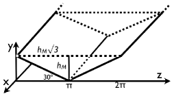
(b) $\beta_{30}(z)$

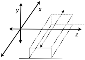
Figure 1: Schematics of straight channels with triangular cross-sections $\Omega$ and coordinate system

Figure 2: Schematics of submerged continental shelf $\beta_{h_{i}}(z)$ and coordinate system.

We consider solutions of the following two forms:

A.

$$\phi(x,y,z,t)=\psi(y,z)\cos(\omega t),$$ (2.8)

referred to as transverse modes see [5], [6].

B.

$$\phi(x,y,z,t)=\psi(y,z)\cos(\kappa x-\omega t),$$ (2.9)

referred to as longitudinal modes, see [5] [29].

We reformulate the problem of finding solutions of the above form in terms of the Dirichlet-Neumann operators.

We first consider transverse modes. Let the fluid domain consist of a straight channel and consider the case $\Omega=\Omega_{B}.$ Consider $f:[0,b]\longrightarrow\mathbb{R}$, and define the Dirichlet-Neumann operator $G_{0}$ by

$$(G_{0}[f])(z)=g\frac{\partial\psi(z,y)}{\partial y}|_{y=0},$$ (2.10)

where $\psi:\Omega\rightarrow\mathbb{R}$ satisfies

$$\left\{\begin{array}[]{l}\Delta\psi=0\text{ }\text{ at }\Omega,\\ \psi(z,y)=f\text{ at }\Omega\cap\Gamma_{F},\\ \frac{\partial\psi}{\partial{\hat{n}}}=0\text{ }\text{ at }\Omega\cap(\Gamma_{B}\cup\Gamma_{L})\\ \end{array}\right.$$ (2.11)

By (2.6)-(2.7), the problem of finding transverse mode solutions (2.8) is then equivalent to solving

$$(G_{0}[f])(z)=\omega^{2}f.$$ (2.12)

Boundary conditions for $f$ must be specified consistently with (2.11). Note that the original formulation (2.6)-(2.7) does not require any boundary conditions on $f$, unless $\Gamma_{L}$ is nonempty, in which case we add Neumann conditions $f_{z}=0$ at $z=0$, $b$.

The operator $G_{0}$ will be approximated by

$$\mathcal{A}_{G_{0}}[f]=\textit{Sym}(D\tanh(h(z)D))[f],$$ (2.13)

using the notation

$$a(z,D)[f](z)=\frac{1}{b}\sum\limits_{k=-\infty}^{\infty}a(z,k)\hat{f}_{k}e^{ik\frac{2\pi}{b}z},$$ (2.14)

$$\hat{f}_{k}=\frac{1}{b}\int_{-{\frac{b}{2}}}^{\frac{b}{2}}f(z)e^{-ik\frac{2\pi}{b}z}dz$$ (2.15)

$\mathcal{A}_{G_{0}}$ is an ad-hoc approximation of $G_{0}$ obtained from the constant depth expression by making $h$ variable, and symmetrizing. $\mathcal{A}_{G_{0}}$ satisfies some basic properties of the exact $G_{0}$, e.g. symmetry, correct high-wavelength asymptotics, see [1], and also has a simple form. As it becomes clearer in the next section the $b-$periodic boundary conditions here are not entirely appropriate. Also, the domains we consider in the next section are symmetric in $z$ so that the eigenfunctions of $\mathcal{A}_{G_{0}}$ are either even or odd, satisfying Neumann and Dirichlet boundary conditions respectively at $z=0$, $b$. This suggests that in the presence of lateral boundaries we should also consider only the even modes as physical.

We now consider longitudinal modes for the case $\Omega_{B}.$ Consider $f(z)=\psi(0,z)$, with $z\in[0,b],$ and define the modified Dirichlet-Neumann operator $G_{\kappa}$ by

$$(G_{\kappa}[f])(z)=g\frac{\partial\psi(z,y)}{\partial y}|_{y=0}$$ (2.16)

where $\psi:\Omega\longrightarrow\mathbb{R}$ satisfies

$$\left\{\begin{array}[]{l}\Delta\psi=\kappa^{2}\psi\text{ }\text{ in }\Omega,\\ \psi(z,y)=f\text{ in }\Omega\cap\Gamma_{F},\\ \frac{\partial\psi}{\partial{\hat{n}}}=0\text{ }\text{ at }\Omega\cap(\Gamma_{B}\cup\Gamma_{L}).\\ \end{array}\right.$$ (2.17)

The problem of finding longitudinal mode solutions (2.9) of (2.6))-(2.7) is equivalent to the spectral problem

$$(G_{\kappa}[f])(z)=\omega^{2}f.$$ (2.18)

Boundary conditions on $f$ are as in the case of transverse modes.

The operator $G_{k}$ of (2.16) will be approximated by the operator

$${\mathcal{A}}_{G_{\kappa}}(\beta)=\textit{Sym}[\sqrt{\kappa^{2}+D^{2}}\tanh(h(z)\sqrt{\kappa^{2}+D^{2}})],\text{ }\text{}$$ (2.19)

with $h(z)=h_{0}-\beta(z)$, $h_{0}=h_{M}-h_{m}>0$ and $D=-i\partial_{z}$ see (2.14). The operator ${\mathcal{A}}_{G_{\kappa}}(\beta)$ is obtained heuristically in the same way as ${\mathcal{A}}_{G_{\kappa}}$, generalizing the case of constant depth.

Longitudinal modes for the case $\Omega_{U}$ lead to (2.17) with $f(z)=\psi(0,z)$, $z\in(-\infty,\infty)$, $\Gamma_{L}=\emptyset$. Solutions of (2.18) that decay at infinity will be referred to it, see [30], [10], [29] for examples in semi-infinite geometry.

${\mathcal{A}}_{G_{\kappa}}(\beta)$ can be also obtained by considering the three dimensional analogue of the approximate Dirichlet-Neumann operator of the previous chapter of the form

$${\mathcal{A}}_{G_{0}}(\beta)=\textit{Sym}[\sqrt{-\Delta}\tanh(h(z)\sqrt{-\Delta})],$$ (2.20)

where $\Delta$ is the Laplacian in $(x,z)$, and $h(z)=-h_{0}+\beta(z)$, $h_{m}=-h_{0}<0$. We note that the depth varies only in the $z$ direction. Generalized eigenfunctions of the operator (2.19) of the form $f(z)e^{\pm i\kappa x}$ lead to the spectral problem for the operator ${\mathcal{A}}_{G_{\kappa}}(\beta)$ of (2.19).

In the next section we describe some known semi-analytic solutions of the form (2.8), (2.9). obtained for special domains with finite cross-section $\Omega$ and $\Gamma_{L}=\emptyset$, i.e. slopping beach geometries. These solutions are constructed starting with a multiparameter family of harmonic functions $\phi_{\mu}$ of the form (2.8), or (2.9), defined on the plane and satisfying the rigid wall boundary condition on a set ${\tilde{\Gamma}}_{B}$ that includes $\Gamma_{B}$ and is the boundary of a domain $\tilde{\mathcal{D}}$ that includes $\mathcal{D}$. Then we require that the $\phi_{\mu}$ also satisfy the first two equations of (2.7) on the free surface $\Gamma_{F}$. This requirement leads to algebraic equations that restrict the allowed values of the parameter $\mu$ to a discrete set and also determine the frequencies. This construction does not assume any boundary conditions for the potential at the free surface.

3 Transverse and longitudinal modes in triangular cross-sections

Transverse and longitudinal modes can be calculated explicitly only for special geometries of the channel cross-sections. In this section we compare some exact results for triangular channels by Lamb [2] Art. 261, Macdonald [3], Greenhill [4], Packham [5], and Groves [6], to results obtained using the non-local operator (2.19).

3.1 Transverse modes for triangular cross-section: $45^{\circ}$ case

The first geometry we consider corresponds to a uniform straight channel with triangular cross-section with a semi-vertical angle $45^{\circ}$, see Figure 3. The cross-section $\Omega=\Omega_{B}$ is as in (2.1) and the bottom is at $y=\beta_{45}(z)$. The minimum and maximum heights of the the fluid domain are $h_{m}=0$ and $h_{M}=\pi$ respectively The channel width is $b=2\pi$, and

$$\beta_{45}(z)=\left\{\begin{array}[]{l}-z+\pi\text{ }\text{ in }0\leq z<\pi\\ z-\pi\text{ }\text{ in }\pi\leq z\leq 2\pi\\ \end{array}\right.,\text{ }z\in[0,2\pi].$$ (3.1)

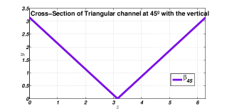
Figure 3: Triangular Cross-section of a straight channel see equation (3.1).

Normal modes for this channel were obtained by Kirchhoff, see Lamb [2], Art. 261, and include symmetric and antisymmetric modes. We review their results:

The symmetric transverse modes, see (2.8), are given by the potential

$$\psi=A[\cosh(\alpha z)\cos(\beta y)+\cos(\beta z)\cosh(\alpha y)]\cos(\omega t).$$ (3.2)

It can be checked that $\frac{\partial\phi}{\partial y}\mid_{y=0}$. Also, $\psi$ is symmetric with respect to the $z=0$ axis, is harmonic in the quarter plane $y\geq|z|$, and satisfies the rigid wall boundary condition

$$\frac{\partial\phi}{\partial\hat{n}}=0\quad\text{at}\quad y=|z|.$$ (3.3)

To impose the boundary condition at the free surface $y=h_{M}$, we use the first two equations of (2.7) to obtain

$$\omega^{2}\psi=\frac{1}{g}\frac{\partial\psi}{\partial y}\quad\text{at}\quad y=h_{M}.$$ (3.4)

Combining with (3.2) we have the conditions

$$\alpha^{2}-\beta^{2}=0,$$ (3.5)

and

$$\omega^{2}\cosh(\alpha h_{M})=g\alpha\sinh(\alpha h_{M}),\quad\omega^{2}\cos(\beta h_{M})=-g\beta\sin(\beta h_{M})=0,$$ (3.6)

or

$$\alpha h_{M}\tanh(\alpha h_{M})+\beta h_{M}\tan(\beta h_{M})=0.$$ (3.7)

The values of $\alpha$, $\beta$ are determined by the intersections of the curves (3.4) and (3.7), see Figure 4(a). There is an infinite number of solutions, $h_{M}\alpha_{j}$, $j=0,2,4,\ldots$, with $\alpha_{j}<\alpha_{j^{\prime}}$ if $j<j^{\prime}$. The corresponding frequencies $\omega_{j}$ are obtained by (3.6). The first values of $h_{M}\alpha_{i},\omega_{i}$ are shown in Table 1. These values are obtained from the intersections of curves (3.9) and (3.11) and of curves (3.4) and (3.7) shown in Figure 4(a) and Figure 4(b) respectively.

To obtain the antisymmetric modes we use the potential

$$\phi=B(\sinh(\alpha z)\sin(\beta y)+\sin(\beta z)\sinh(\alpha y))\cos(\omega t).$$ (3.8)

We check that $\phi$ satisfies the rigid wall boundary conditions at $y=|z|$ and is harmonic in the quadrant $y\geq|z|$. We also check that $\frac{\partial\phi}{\partial y}\mid_{y=0}$ is antisymmetric with respect to the $z=0$ axis. Imposing the free surface boundary conditions (2.7) to (2.8) we obtain (3.4). Then (3.8) leads to the conditions

$$\alpha^{2}-\beta^{2}=0$$ (3.9)

and

$$\omega^{2}\sinh(\alpha h_{M})=g\alpha\cosh(\alpha h_{M}),\quad\omega^{2}\sin(\beta h_{M})=g\beta\cos(\beta h_{M}),$$ (3.10)

or

$$\alpha h\coth(\alpha h_{M})=\beta h_{M}\cot(\beta h_{M}).$$ (3.11)

The values of $\alpha$, $\beta$ are determined by the intersections of the curves (3.9) and (3.11), see Figure 4(b). There is an infinite number of solutions $h_{M}\alpha_{j}$, $j={1,3,5...}$ with $\alpha_{j}<\alpha_{j^{\prime}}$ if $j<j^{\prime}$. The corresponding frequencies $\omega_{j}$ are given by (3.10), see Table 1.

By (2.7) the free surface corresponding to the above symmetric and antisymmetric modes is computed by

$$\eta(z)=\frac{1}{g}\frac{\partial\phi}{\partial y}\mid_{y=h_{M}}.$$ (3.12)

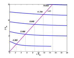
(a) Even modes

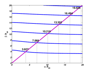
(b) Odd modes

Figure 4: (a) Intersection of curves (3.9) and (3.11). (b) Intersection of curves: (3.4) and (3.7).

Table 1: Frequencies of modes for channel of Figure 3

	$i=0$	$i=1$	$i=2$	$i=3$	$i=4$	$i=5$	$\cdots$
$\alpha_{i}h_{M}$	2.365	3.927	5.498	10.210	11.781	16.494	$\cdots$
$\omega_{i}$	4.8624	7.8261	4.1413	5.6445	6.0622	7.1684	$\cdots$

In Figure 5 and Figure 6 we compare the surface amplitude of the exact symmetric and antisymmetric modes found above to the surface amplitudes obtained by computing numerically the eigenfunctions of the approximate Dirichlet-Neumann operator ${\mathcal{A}}_{G_{0}}(\beta)$ of (2.13) with $2\pi-$periodic boundary conditions. The operator is discretized spectrally. Given a computed eigenfunction $f$ of ${\mathcal{A}}_{G_{0}}(\beta)$ we obtain the surface amplitude $\eta$ by $\eta=\frac{1}{g}\mathcal{A}_{G_{k}}(\beta)$. This is analogous to (3.12).

Figure 5 suggests good quantitative agreement for the even modes. For the odd modes we see that the wave amplitudes differ at the boundary representing the sloping beach. In particular the odd eigenvectors of ${\mathcal{A}}_{G_{\kappa}}(\beta)$ have nodes at $z=0$, $b=2\pi$, while the exact odd modes do not. The procedure for obtaining the exact modes does not require any conditions on the value of the potential at the intersection of the free boundary and the rigid wall. Also, the free surface is described by a value of the $y-$coordinate, and this allows us to define $\eta(z)$ for all real $z$, in particular we determine the fluid domain by computing the intersection of the graph of $\eta$ with the rigid wall. This leads to a more realistic motion of the surface at the sloping beach, although this does not imply that the exact solutions are physical either, since the boundary conditions at the free surface are not exact. In contrast, the odd modes of ${\mathcal{A}}_{G_{\kappa}}(\beta)$ correspond to pinned boundary conditions that are not expected to be physical.

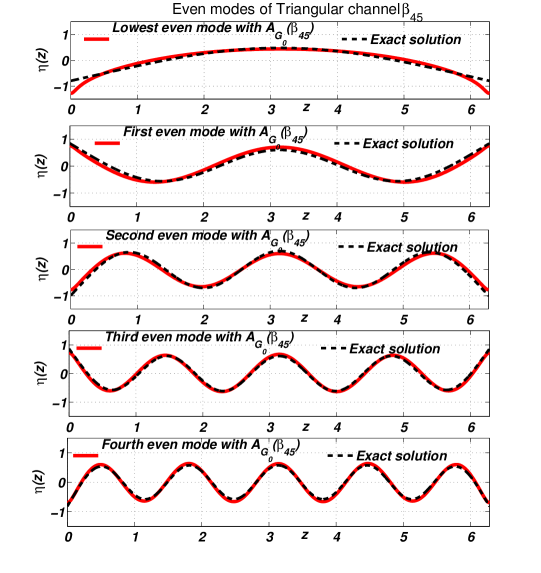
Figure 5: Symmetric transverse modes of a channel with triangular cross section illustrated in Figure 3. Red (solid) lines: operator $\mathcal{A}_{G_{0}}$, dashed lines: exact solutions from (3.2) and the values in Table 1.

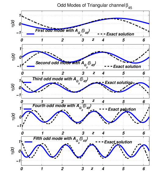
Figure 6: Antisymmetric transverse modes of a channel with triangular cross section illustrated in Figure 3. Blue (solid) lines: operator $\mathcal{A}_{G_{0}}$, dashed lines: exact solutions using (3.8) and the values in Table 1.

3.2 Longitudinal modes for triangular cross-sections: $60^{\circ}$ case

A second geometry with exact longitudinal modes was considered by Macdonald [3], Packham, [5], see also Lamb [2], Art. 261. This geometry corresponds to a uniform straight channel with triangular cross-section with a semi vertical angle $60^{\circ}$, as illustrated in Figure 7. In this case we will examine longitudinal modes.

We consider the cross-section $\Omega=\Omega_{B}$, as in (2.1) and the bottom $\beta_{30}(z)$. The channel width is $b=2\pi$ and the maximum and minimum heights of the fluid domain are $h_{M}=\frac{\pi}{\sqrt{3}}$ and $h_{m}=0$ respectively. The cross-section profile is given by

$$\beta_{30}(z)=\left\{\begin{array}[]{l}\frac{-1}{\sqrt{3}}z+\frac{\pi}{\sqrt{3}}\text{ }\text{ in }0\leq z<\pi\\ \frac{1}{\sqrt{3}}z-\frac{\pi}{\sqrt{3}}\text{ }\text{ in }\pi\leq z\leq 2\pi\\ \end{array}\right.,\text{ }z\in[0,2\pi].$$ (3.13)

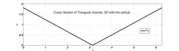
Figure 7: Triangular cross-section of a straight channel, see equation (3.13).

The exact solutions for symmetric modes, see Packham [5], and Groves [6] are the following.

The $0-$mode is described by a velocity potential $\phi$ of the form (2.9) with

$$\psi(z,y) = A[\cosh(\kappa(y-h_{M}))+\frac{\omega^{2}\kappa^{2}}{g\kappa}\sinh(\kappa(y-h_{M}))$$

$$+2\cosh(\frac{\sqrt{3}\kappa(z-\pi)}{2})$$

$$\times\{\cosh(\kappa(\frac{y}{2}+h_{M}))-\frac{\omega^{2}\kappa^{2}}{g\kappa}\sinh(\kappa(\frac{y}{2}+h_{M}))\}],$$

and

$$\omega^{2}=\frac{3g}{4\kappa}\coth(\frac{3\kappa h_{M}}{2})\{1+(1-\frac{8}{9}\tanh^{2}(\frac{3\kappa h_{M}}{2}))^{\frac{1}{2}}\}.$$ (3.15)

The remaining symmetric modes $2,4,6,8,...$ are described by a velocity potential $\phi$ of the form (2.9) with

$$\psi = A[\{\cosh(\alpha(y-h_{M}))+\frac{\omega^{2}\kappa^{2}}{g\kappa}\sinh(\alpha(y-h_{M}))\}\cos(\beta(z-\pi))$$

$$+2\cosh(\frac{\sqrt{3}\alpha(z-\pi)}{2})\cos(\frac{\sqrt{3}\beta y}{2})\cos(\frac{\beta(z-\pi)}{2})$$

$$\times\{\cosh(\alpha(\frac{y}{2}+h_{M}))-\frac{\omega^{2}\kappa^{2}}{g\kappa}\sinh(\alpha(\frac{y}{2}+h_{M}))\}$$

$$-2\sinh(\frac{\sqrt{3}\alpha(z-\pi)}{2})\sin(\frac{\sqrt{3}\beta y}{2}\sin(\frac{\beta(z-\pi)}{2}))$$

$$\times\{\sinh(\alpha(\frac{y}{2}+h_{M}))-\frac{\omega^{2}\kappa^{2}}{g\kappa}\cosh(\alpha(\frac{y}{2}+h_{M}))\}],$$

$$\omega^{2}=\frac{g\alpha}{\kappa^{2}}\left[\frac{\frac{\beta}{\alpha}\sqrt{3}(\cosh(3\alpha h_{M})-\cos(\sqrt{3}\beta h_{M}))}{\frac{\beta}{\alpha}\sqrt{3}\sinh(3\alpha h_{M})-3\sin(\sqrt{3}\beta h_{M})}\right].$$ (3.17)

The above potentials are harmonic and satisfy the rigid wall boundary conditions. The first two equations of motion (2.7) lead to

$$\alpha^{2}-\beta^{2}=\kappa^{2},$$ (3.18)

and

$$\left(\frac{\beta}{\alpha}\right)^{2}\cosh(3\alpha h_{M})\cos(\sqrt{3}\beta h_{M})$$

$$- \frac{1}{4}\left(\frac{\beta}{\alpha}\right)\sqrt{3}\left\{1-\left(\frac{\beta}{\alpha}\right)^{2}\right\}\sinh(3\alpha h_{M})\sin(\sqrt{3}\beta h_{M})$$

$$-\frac{1}{4}\left[\left\{3+5\left(\frac{\beta}{\alpha}\right)^{2}\right\}-\left\{3+\left(\frac{\beta}{\alpha}\right)^{2}\right\}\cos^{2}(\sqrt{3}\beta h_{M})\right]=0.$$

In Figure 9 we show the symmetric longitudinal modes derived with the values of $\alpha$ and $\beta$ obtained from relations (3.18) and 3.2 for $\kappa=2$, see also Table 2.

By (2.7) the free surface corresponding to the above symmetric and antisymmetric modes is computed by

$$\eta(z)=\frac{1}{g}\frac{\partial\phi}{\partial y}\mid_{y=h_{M}}.$$

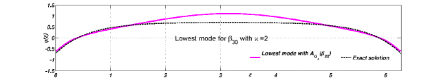
Figure 8: Lowest longitudinal mode with $\kappa=2$ given by (3.2) and (3.15) for the triangular channel illustrated in Figure 7.

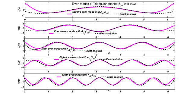
Figure 9: Symmetric longitudinal modes: $2$, $4$, $6$, $8$, $10$ of a channel with triangular cross section illustrated in Figure 7. Magenta (solid) lines: operator $\mathcal{A}_{G_{\kappa}}(\beta_{30})$ with $\kappa=2$, dashed lines: exact solutions given by (3.2) and (3.17) and the values in Table 2.

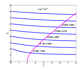
Figure 10: Graphs for the determination of $\alpha$ and $\beta$ for the modes $2$, $4$, $6$, $8$, and $10$ using $\kappa=2$, $h_{M}=\frac{\pi}{\sqrt{3}}$.

Table 2: Frequencies of modes of channel of Figure 7

	$i=2$	$i=4$	$i=6$	$i=8$	$i=10$	$\cdots$
$\alpha_{i}$	2.409	3.146	3.996	4.900	5.836	$\cdots$
$\beta_{i}$	1.343	2.429	3.460	4.474	5.482	$\cdots$
$\omega_{i}$	2.4297	2.7764	3.1289	3.4651	3.7813	$\cdots$

These values are associated to graphic roots in Figure 10 for the geometry with the cross-section of Figure 7, see (3.13). We use $h_{M}=\frac{\pi}{\sqrt{3}}.$

In Figures 8 and 9 we compare the surface amplitude of the exact symmetric modes with the surface amplitudes obtained by computing numerically the eigenfunctions of the approximate Dirichlet-Neumann operator ${\mathcal{A}}_{G_{\kappa}}(\beta)$ of (2.20) with $\beta$ as in (3.13). We use $\kappa=2$. To compute the eigenfunctions of ${\mathcal{A}}_{G_{\kappa}}(\beta)$ numerically we use $2\pi-$periodic boundary conditions. Also, given a computed eigenfunction $f$ the surface amplitude $\eta$ is given by $\eta=\frac{1}{g}\mathcal{A}_{G_{k}}(\beta)$. This is analogous to (3.12).

Figure 9 shows good quantitative agreement for the even modes in the interior, with some discrepancies at the boundary that represents the sloping beach.

To our knowledge there are no exact solutions reported in the literature for odd modes. Odd modes obtained with the approximate Dirichlet-Neumann operator are shown in Figure 11. The results on the isosceles triangle of angle $45^{\circ}$ suggest that the solutions should be accurate far from the boundary.

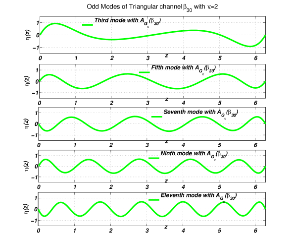
Figure 11: Odd longitudinal modes: $3$, $5$, $7$, $9$ derived from operator $\mathcal{A}_{G_{\kappa}}(\beta_{\beta_{30}})$ with $\kappa=2$ for straight channel with triangular cross-section illustrated in Figure 7.

We have also used the approximate Dirichlet-Neumann operator to compute the $2\pi-$periodic normal modes of domains obtained from the triangular channel by adding an interval of extra depth, see Figure 12. We denote the added depth by $T$. Figure 13, and Figure 14 indicate the convergence to the triangular domain modes as $T$ vanishes. In this geometry even modes satisfy a Neumann boundary condition at $z=0$, $2\pi$, and $T$ can be interpreted also as the height of a vertical wall.

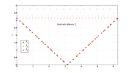
Figure 12: Cross section of the straight channels with lateral boundary $\Gamma_{L}$. Vertical segments of height $T_{1}=0.006$ (red), $T_{2}=0.15$ (green), $T_{3}=.6$ (magenta).

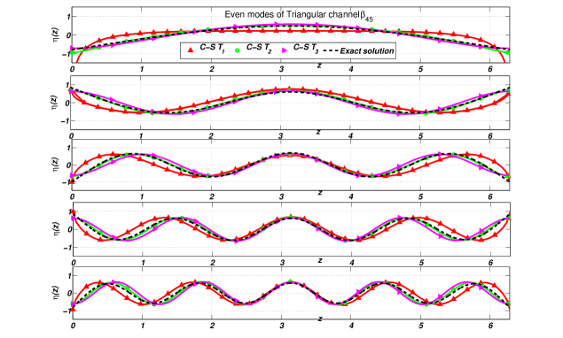
Figure 13: Even modes for the three cross sections of Figure 12, vertical segments of heights $T_{1}=.006$ (red), $T_{2}=.15$ (green) , $T_{3}=.6$ (magenta).

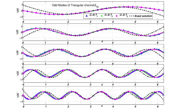
Figure 14: Odd modes for the three cross sections of Figure 12 vertical segments of heights $T_{1}=.006$ (red), $T_{2}=.15$ (green) , $T_{3}=.6$ (magenta).

4 Trapped modes over continental shelf profiles

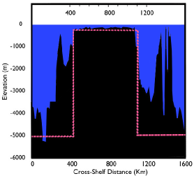
(a) Off coast of Taiwan.

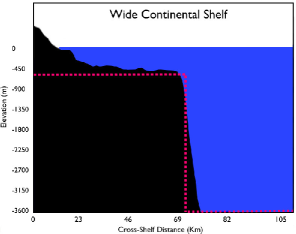
(b) Coast of California.

Figure 15: a) Typical topographic profile of shelf at distance of $50km$ from the coast of Taiwan, [8] . b) Typical topographic profile of California coast, [9, 7].

In this section we study a model problem of waves that travel along a continental shelf and decay in the transverse direction. These are examples of longitudinal modes (2.9) and we use a two-valued piecewise constant transverse depth profile $\Omega_{U}$, see (2.2). We will compare results from two approximations of the linear water wave system (2.7). The first is a variable depth version of the linear shallow water equation, where the spectral problem for piecewise constant depth is reduced to solving algebraic equations, see Miles [7], Lin, Juang and Tsay [8], and [9]. These studies model continental shelves off the coasts of California and Taiwan respectively, and we will use the same parameters. The second approximation is the linear Whitham-Boussinesq equation [1], whose longitudinal modes lead to the spectral problem for the model Dirichlet-Neumann ${\mathcal{A}}_{G_{\kappa}}(\beta)$ of (2.19). The numerical eigenfunctions of this operator are compared with the trapped modes obtained with the shallow water theory.

The problem considered in the literature [7, 8, 9] for the shallow water model is not the usual spectral problem of fixing $\kappa$ and finding $\omega$ in (2.9), rather the authors fix $\omega$ (determined by observations) and look for values of $\kappa$ leading to solutions that decay in the transverse direction (trapped modes). We compare these modes to numerical eigenfunctions of ${\mathcal{A}}_{G_{\kappa}}(\beta)$ with the $\kappa$ obtained from the shallow water problem.

The continental shelves will be modeled by domains of the form $\Omega_{U}$, see (2.2), with a depth that is constant in the longitudinal direction $x$ and only depends on the transverse direction $z$. The simplest model of a continental shelf is a plateau of constant depth $h_{2}$ in an interval of length $2a$, and $h_{1}>h_{2}$ for all other $z$. e.g. $h_{M}=-h_{1}$, $h_{m}=0$ in the notation of Section 2.

4.1 Exact trapped modes solutions over continental shelves with shallow water theory.

We outline the linear shallow water theory of [7], [9], and [8]. The linear shallow water wave equation is

$$g\nabla\cdot(h(z)\nabla\eta)=\frac{\partial^{2}\eta}{\partial t^{2}},$$ (4.1)

with $\nabla=(\partial_{x},\partial_{z})$. The function $h$ is the depth. We are looking for longitudinal wave solutions of the form

$$\eta(x,z,t)=V(z)\cos(\kappa x-\omega t),$$ (4.2)

see (2.9). By (4.2), (4.1) we have

$$-\frac{\partial}{\partial z}\left(h(z)\frac{\partial V(z)}{\partial z}\right)+h(z)\kappa^{2}V(z)=\frac{\omega^{2}}{g}V(z),$$ (4.3)

Assuming $h(z)$ piecewise constant with

$$h(z)=\left\{\begin{array}[]{l}h_{2}\text{ for }z\in[-a,a],\\ h_{1}\text{ for }z\notin[-a,a],\\ \end{array}\right.$$ (4.4)

(4.3) becomes

$$gh_{j}\frac{\partial^{2}V}{\partial z^{2}}+V\omega^{2}=\kappa^{2}gh_{j}V,$$ (4.5)

with $j=1,2$. We fix $\omega$ and solve the equation in each region. At each constant depth we have

$$\frac{\partial^{2}V}{\partial z^{2}}=(\kappa^{2}-\lambda_{j}^{2})V,\quad\hbox{with}\quad\lambda_{j}=\frac{\omega}{\sqrt{gh_{j}}},$$ (4.6)

with $j=1,2$. Clearly, we have two kinds of solutions:

• Oscillatory solutions. If $\lambda^{2}\geq\kappa^{2}$, then

  $$V(z)=Be^{i\alpha z}+Ce^{-i\alpha z},\quad\text{where}\quad\alpha=\sqrt{\lambda^{2}-\kappa^{2}}.$$ (4.7)

• Exponentially growing/decaying solutions. If $\lambda^{2}\leq\kappa^{2}$, then

  $$V(z)=Ae^{\gamma z}+De^{-\gamma z},\quad\text{where}\quad\gamma=\sqrt{\kappa^{2}-\lambda^{2}}.$$ (4.8)

We seek solutions that are oscillatory for $z\in[-a,a]$, decay exponentially for $z\notin[-a,a]$, and lead to continuous $\eta$ and $h(z)\frac{\partial\eta}{\partial z}$. The continuity condition requires that that $V$, and $h(z)V$ be continuous at $z=a$, $-a$. Note that the continuity condition guaranties that the solution is a weakly differentiable function.

By the symmetry of the equation and the domain it is enough to look for even and odd real solutions. Even solutions are given by

$$V(z)=B\cos(\alpha_{2}z),\text{ }\text{ }z\in[-a,a],$$ (4.9)

with

$$\alpha_{2}=\sqrt{\lambda_{2}^{2}-\kappa^{2}},\quad\lambda_{2}=\frac{\omega}{\sqrt{gh_{2}}},$$ (4.10)

and

$$V(z)=Ae^{-\gamma_{1}(\mid z\mid-a)},\text{ }\text{ }z\notin[-a,a],$$ (4.11)

with

$$\gamma_{1}=\sqrt{\kappa^{2}-\lambda_{1}^{2}},\quad\lambda_{1}=\frac{\omega}{\sqrt{gh_{1}}}.$$ (4.12)

Odd solutions are given by

$$V(z)=B^{\prime}\sin(\alpha_{2}z)\text{ }\text{ at }z\in[-a,a]\text{ and }h(z)=h_{2},$$ (4.13)

with $\alpha_{2}$, $\lambda_{2}$ as in (4.10), and

$$V(z)=-A^{\prime}e^{-\gamma_{1}(\mid z\mid-a)}\text{ }\text{ at }z\notin[-a,0]\text{ and }h(z)=h_{1},$$ (4.14)

$$V(z)=A^{\prime}e^{-\gamma_{1}(\mid z\mid-a)}\text{ }\text{ at }z\notin[0,a]\text{ and }h(z)=h_{1},$$ (4.15)

with $\gamma_{1}$, $\lambda_{1}$ as in (4.12).

Requiring continuity of $\eta$ and $h(z)\frac{\partial\eta}{\partial z}$ at $z=\pm a$ we have the following.

For the even modes, (4.9)-(4.12) imply

$$B\cos(\alpha_{2}a)=A,$$ (4.16)

$$-h_{2}B\alpha_{2}\sin(\alpha_{2}a)=-h_{1}\gamma_{1}A,$$ (4.17)

which imply

$$\tan(\alpha_{2}a)=\frac{h_{1}\gamma_{1}}{h_{2}\alpha_{2}}.$$ (4.18)

We thus obtain an equation for $\alpha_{2}$ and $\gamma_{1}$. This equation can not be solved analytically. We thus search for a solution graphically (i.e. numerically). To do so, we first let

$$\chi=a\sqrt{\lambda_{2}^{2}-\kappa^{2}}=a\alpha_{2},\quad h=\frac{h_{2}}{h_{1}}.$$ (4.19)

Then we can rewrite equation (4.18) as

$$\tan(\chi)=\frac{\sqrt{\kappa^{2}-\lambda_{1}^{2}}}{h\alpha_{2}}.$$

Note that $\lambda_{1}^{2}=h\lambda_{2}^{2}$, and that

$$a\sqrt{\kappa^{2}-h\lambda_{2}^{2}}=\sqrt{a^{2}\kappa^{2}-a^{2}h\lambda_{2}^{2}} = \sqrt{\lambda_{2}^{2}a^{2}(1-h)-\chi^{2}},$$ (4.20)

so that letting

$$\chi_{*}^{2}=\frac{(\omega a)^{2}}{gh_{2}}(1-h),$$ (4.21)

we must solve

$$\cot\chi=\frac{h\chi}{\sqrt{\chi_{*}^{2}-\chi^{2}}}.$$ (4.22)

Continuity of the odd solutions leads to

$$B^{\prime}\sin(\alpha_{2}a)=A^{\prime},$$ (4.23)

$$h_{2}B^{\prime}\alpha_{2}\cos(\alpha_{2}a)=-h_{1}\gamma_{1}A’,$$ (4.24)

implying

$$\cot(\alpha_{2}a)=-\frac{h_{1}\gamma_{1}}{h_{2}\alpha_{2}}.$$ (4.25)

Using the above notation this is equivalent to

$$\tan\chi=-\frac{h\chi}{\sqrt{\chi_{*}^{2}-\chi^{2}}}.$$ (4.26)

The numerical solutions of (4.22), (4.26) are shown in (4.25), (4.26) and in Tables 3 and 4.

4.2 Trapped modes on idealized shelves off California and Taiwan coasts

Shelf off coast of California. The first example we consider models the continental shelf off the coast of California following [7], [9]. The depth topography is described by $h_{2}=600$ m, $h_{1}=3600$ m, and total shelf length $2a=140$ km, Figure 15(b). We compute both even and odd trapped modes, but by the geometry of Figure 15(b) we only consider the even ones, restricted to $z>0$, as physical.

In our computations we rescale, using $h_{1}=1$ so that $h_{2}=\frac{1}{6}=0.1617$. The rescaled total shelf length is $2a=12\pi$, see (4.27) for the corresponding cross-section in Figure 16. In the notation of Section 2, $h_{M}=h_{1}$, $h_{m}=0$, and the bottom is at $y=h_{m}+\beta(z)$ with

$$\beta(z)=\beta_{\text{Off-California}}(z)=\left\{\begin{array}[]{l}0\text{ in }-\infty\leq z<10\pi,\\ 5/6\text{ in }10\pi\leq z\leq 22\pi,\\ 0\text{ in }22\pi\leq z<\infty.\\ \end{array}\right.$$ (4.27)

The numerical eigenfunctions of the operator ${\mathcal{A}}_{G_{\kappa}}(\beta)$ of (2.19) are computed using the domain $[0,32\pi]$, with periodic boundary conditions.

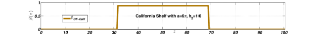
Figure 16: California shelf, see (4.27).

Shelf off coast of Taiwan. This continental shelf is located off the eastern coast of Taiwan, on the edge of the continental shelf of Asia. Off the edge of the shelf the slope plunges down to the deep Pacific Ocean, at a gradient of 1:10 and the ocean reaches a depth of more than 5000 meters about 50 kilometers off the coast, as shown in Figure 15(a). An idealized model for this shelf by Lin, Juang and Tsay [8] uses $h_{2}=80m$ on the shelf, $h_{1}=5000m$ on both sides of the ridge and total shelf length of $2a=650km$, see Figure 15(a), [8].

After rescaling, we consider a fluid domain with depth $h_{1}=1$, obtaining $h_{2}=.0160$ over the ridge and a total shelf length is $2a=130$, see (4.28) for the corresponding cross-section as shown Figure 21. In the notation of Section 2, $h_{M}=h_{1}$, $h_{m}=0$, and the bottom is at $y=h_{m}+\beta(z)$ with

$$\beta(z)=\beta_{\text{Off-Taiwan}}(z)=\left\{\begin{array}[]{l}0\text{ in }-\infty\leq z<25\pi,\\ 24/25\text{ in }25\pi\leq z\leq 65\pi,\\ 0\text{ in }65\pi\leq z<\infty.\\ \end{array}\right.$$ (4.28)

The numerical eigenfunctions of the operator ${\mathcal{A}}_{G_{\kappa}}(\beta)$ of (2.19) are computed using the domain $[0,90\pi]$, with periodic boundary conditions.

I. California shelf We use the data of [7] to compute $\chi_{*}=6.8801\approx 2.19\pi$, $\omega=0.1582$. From the graphical solutions shown in the lower plot of Figure 17 for $n$ even we see that for $\chi_{*}=2.19\pi$ we have three points of intersection: $0<\chi_{0}<\pi<\chi_{2}<2\pi<\chi_{4}<\chi_{*}<3\pi$. From the graphical solution in the upper plot of the same figure for $n$ odd we see that for $\chi_{*}=2.19\pi$ there are two points of intersection: $\frac{\pi}{2}<\chi_{1}<\frac{3\pi}{2}<\chi_{3}<\frac{5\pi}{2}$. We thus have five trapped modes. In Table 3 we summarize the values $\chi_{i}$ obtained from the intersection of the curves.

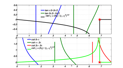
Figure 17: Upper side shows graphical solution of (4.26) for odd modes of Off Coast of California and lower side shows graphical solution of (4.22) for even modes. Red star corresponds to $\chi_{*}=2.19\pi$

In Table 4 we show the values of $\kappa_{n}$ and $\gamma_{1_{n}}$ for $n=0,\dots,4$. The surface amplitude of each mode, see (4.2), (4.9)-(4.15), is shown in Figure 18.

Table 3: The roots $\chi_{n}$ of (4.22), (4.26)

	$\chi_{0}$	$\chi_{1}$	$\chi_{2}$	$\chi_{3}$	$\chi_{4}$
Even	1.5327		4.5656		6.8429
Odd		3.059		5.9954

Table 4: Wavenumbers $\alpha_{n}$, see (4.19) associated to the roots $\chi_{n}$

	$n=0$	$n=1$	$n=2$	$n=3$	$n=4$
$\alpha_{2_{n}}=\frac{\chi_{n}}{a}$	0.0813	0.1623	0.2422	0.3181	0.3630
$\kappa_{n}=\sqrt{\lambda_{2}^{2}-\alpha_{2_{n}}^{2}}$	0.6271	0.6111	0.5841	0.5465	0.5177
$\gamma_{1_{n}}=\sqrt{\kappa_{n}^{2}-\lambda_{1}^{2}}$	0.7460	0.7326	0.7102	0.6796	0.6567

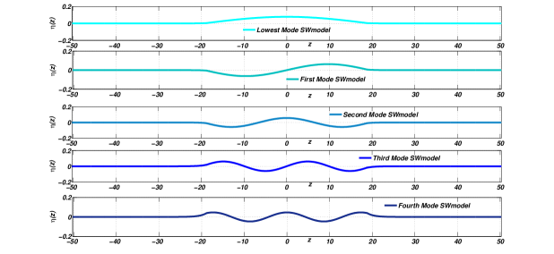
Figure 18: Surface profiles of trapped modes derived with formulas (4.9) and (4.13) for the Coast of California, see (4.27), Figure 16.

To compare to the modes obtained using the operator ${\mathcal{A}}_{G_{\kappa}}(\beta)$, we let $\kappa=\kappa_{n}$, with $n=0,\ldots,4$, and for each value $\kappa=\kappa_{n}$ compute the corresponding eigenvalues and eigenvectors. We compare the $n-$ th eigenvector of $\mathcal{A}_{G_{\kappa_{n}}}$ to the shallow water mode corresponding to $\kappa_{n}$. The modes obtained are shown in (19), together with the modes obtained using the shallow water modes. We see that the two results are close, especially for the lowest modes.

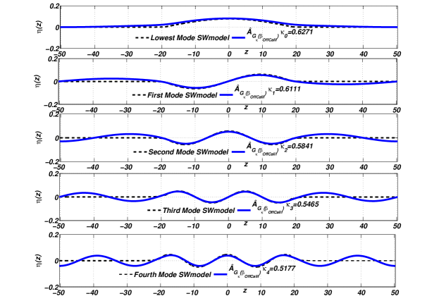
Figure 19: Comparisons of amplitude profiles of normal modes obtained by shallow water theory in dashed lines and eigenfunctions of operator $\mathcal{A}_{G_{\kappa_{n}}}(\beta_{OffCalif})$ in solid lines. The figures from the top to the bottom shows: in blue line the surface profiles derived from operator$\mathcal{A}_{G_{\kappa_{n}}}(\beta_{OffCalif})$ for $n=0$, $\kappa_{0}=0.6271$, for $n=1$, $\kappa_{1}=0.6111$, $n=2$, $\kappa_{2}=0.5841$, for $n=3$, $\kappa_{3}=0.5465$, $n=4$, $\kappa_{4}=0.5177$.

II. Taiwan shelf In this example we follow [8], obtaining $\chi_{*}=1.618$, $\omega=0.0165$. The graphical solution shown in Figure 20 indicates that there is only one trapped even mode with $\chi_{0}=1.4804$ and $\kappa=\kappa_{0}=0.1604$, see Table 5. This mode is shown in in Figure 22, where we also plot the lowest frequency mode of ${\mathcal{A}}_{G_{\kappa}}(\beta)$. We observe that the two modes are close to each other.

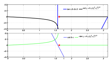
Figure 20: Graphical solution of (4.26) for odd modes of Off Coast of Taiwan and lower side shows graphical solution of (4.22) for even modes. Red star corresponds to $\chi_{*}=1.618$.

Table 5: Wavenumber $\alpha_{0}$, see (4.19) associated to the root $\chi_{0}$

	$\alpha_{2_{0}}$	$\kappa_{0}$	$\gamma_{1_{0}}$
$n=0$	0.0236	0.1604	0.1760

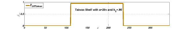
Figure 21: Taiwan shelf, see (4.28).

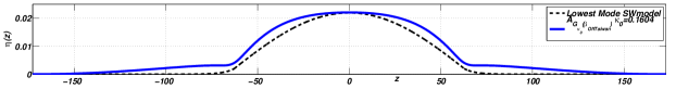
Figure 22: Comparisons of amplitude profile of normal mode obtained by shallow water theory in dashed line and eigenfunction of operator $\mathcal{A}_{G_{\kappa_{0}}}(\beta_{OffTaiwan})$ for $n=0$, $\kappa_{0}=0.1604.$ in solid line.

5 Discussion

We have studied two problems on linear water wave modes in channels with variable depth, choosing depth geometries and models with known exact results. The main goal was to test a nonlocal version of dispersive shallow water theory that uses a simple nonlocal approximation of the Dirichlet-Neumann operator for variable depth. The approximate Dirichlet-Neumann operator we use leads to a unified and relatively simple way to compute numerically normal modes for variable depth channels. Our results on normal modes in bounded domains indicate that this operator can give reasonable approximations, even though geometries with exact normal modes have sloping beaches and seem to pose too stringent a test for the nonlocal operator. This is because our operator is most naturally defined on periodic functions and the symmetry of the depth profile imposes boundary conditions that are not present in the exact formulation of the normal mode problem. Despite this issue, the two approaches lead to normal modes that are close away from the boundary. The main discrepancies are seen near the sloping beach for odd modes. These discrepancies motivate some further study on how to best use or extend the Dirichlet-Neumann approach for sloping beach problems. The operator used here was an ad-hoc approximation, but the boundary conditions problem seems relevant to more systematic approximations of the exact Dirichlet-Neumann operator, e.g. the ones in [16, 18].

The problem of trapped modes for unbounded domains was studied using linear St. Venant shallow water theory. Despite the simplifications it introduces, shallow water theory has given some useful insights into the behaviour of trapped modes in other contexts, e.g. Ursell modes in semi-infinite sloping beach domains and their excitation by incoming waves [31, 32, 10, 11]. Also, geophysical applications motivate simplified models that combines features of the both the St. Venant and variable depth Whitham-Boussinesq equations and it is therefore natural to compare the two models. However, the present study of the spectral problem for the transverse modes of the nonlocal linear equations is limited to reproducing results of the St. Venant theory, and is mainly indicative of the possible geophysical interest of the variable depth Whitham-Boussinesq equations. We are currently working on ways to determine the number of trapped modes of the operator $\mathcal{A}_{G_{\kappa}}$ for the continental shelf and similar depth topographies, some related results are in [31, 32, 29]. It would be also of interest to consider nonlinear effects on the modes discussed in this paper.

References

- [1] RM Vargas-Magaña and P Panayotaros. A whitham–boussinesq long-wave model for variable topography. Wave Motion, 65:156–174, 2016.
- [2] Horace Lamb. Hydrodynamics. Cambridge university press, 1932.
- [3] HM Macdonald. Waves in canals. Proceedings of the London Mathematical Society, 1(1):101–113, 1893.
- [4] AG Greenhill. Wave motion in hydrodynamics (continued). American Journal of Mathematics, pages 97–112, 1887.
- [5] BA Packham. Small-amplitude waves in a straight channel of uniform triangular cross-section. The Quarterly Journal of Mechanics and Applied Mathematics, 33(2):179–187, 1980.
- [6] MARK D GROVES. Hamiltonian long-wave theory for water waves in a channel. Quarterly journal of mechanics and applied mathematics, 47:367–404, 1994.
- [7] John W Miles. Wave propagation across the continental shelf. Journal of Fluid Mechanics, 54(01):63–80, 1972.
- [8] Ming-Chung Lin, Wen-Jye Juang, and Ting-Kuei Tsay. Anomalous amplifications of semidiurnal tides along the western coast of taiwan. Ocean Engineering, 28(9):1171–1198, 2001.
- [9] Chiang C Mei, Michael Stiassnie, and Dick K-P Yue. Theory and applications of ocean surface waves: nonlinear aspects, volume 23. World scientific, 2005.
- [10] Anne-Sophie BONNET and Patrick JOLY. Mathematical and numerical study of trapping waves. In Fifth Zntl. Workshop on Water Waves and Floating Bodies, Manchester, pages 25–28, 1990.
- [11] DS Kuznetsov. A spectrum perturbation problem and its applications to waves above an underwater ridge. Siberian Mathematical Journal, 42(4):668–684, 2001.
- [12] Vladimir E Zakharov. Stability of periodic waves of finite amplitude on the surface of a deep fluid. Journal of Applied Mechanics and Technical Physics, 9(2):190–194, 1968.
- [13] AC Radder. An explicit hamiltonian formulation of surface waves in water of finite depth. Journal of Fluid Mechanics, 237:435–455, 1992.
- [14] John W Miles. On hamilton’s principle for surface waves. Journal of Fluid Mechanics, 83(01):153–158, 1977.
- [15] Walter Craig and Mark D Groves. Hamiltonian long-wave approximations to the water-wave problem. Wave motion, 19(4):367–389, 1994.
- [16] Walter Craig, Philippe Guyenne, David P Nicholls, and Catherine Sulem. Hamiltonian long–wave expansions for water waves over a rough bottom. In Proceedings of the Royal Society of London A: Mathematical, Physical and Engineering Sciences, volume 461, pages 839–873. The Royal Society, 2005.
- [17] David Lannes. The water waves problem. Mathematical surveys and monographs, 188, 2013.
- [18] Maïté Gouin, Guillaume Ducrozet, and Pierre Ferrant. Development and validation of a highly nonlinear model for wave propagation over a variable bathymetry. In ASME 2015 34th International Conference on Ocean, Offshore and Arctic Engineering, pages V007T06A077–V007T06A077. American Society of Mechanical Engineers, 2015.
- [19] Numerical study of a nonlocal model for water-waves with variable depth. Wave Motion, 50(1):80 – 93, 2013.
- [20] Daulet Moldabayev, Henrik Kalisch, and Denys Dutykh. The whitham equation as a model for surface water waves. arXiv preprint arXiv:1410.8299, 2014.
- [21] Mats Ehrnström, Henrik Kalisch, et al. Traveling waves for the whitham equation. Differential and Integral Equations, 22(11/12):1193–1210, 2009.
- [22] Mats Ehrnström, Mark D Groves, and Erik Wahlén. On the existence and stability of solitary-wave solutions to a class of evolution equations of whitham type. Nonlinearity, 25(10):2903, 2012.
- [23] Pavel Ivanovich Naumkin and Ilʹi︠a︡ Andreevich Shishmarev. Nonlinear nonlocal equations in the theory of waves. Amer Mathematical Society, 1994.
- [24] Adrian Constantin and Joachim Escher. Wave breaking for nonlinear nonlocal shallow water equations. Acta Mathematica, 181(2):229–243, 1998.
- [25] Vera Mikyoung Hur. Breaking in the whitham equation for shallow water waves. arXiv preprint arXiv:1506.04075, 2015.
- [26] Mats Ehrnstrom and Erik Wahlén. On whitham’s conjecture of a highest cusped wave for a nonlocal dispersive equation. arXiv preprint arXiv:1602.05384, 2016.
- [27] DV Evans and CM Linton. Sloshing frequencies. The Quarterly Journal of Mechanics and Applied Mathematics, 46(1):71–87, 1993.
- [28] Gerald Beresford Whitham. Linear and nonlinear waves, volume 42. John Wiley & Sons, 2011.
- [29] N Kuznetsov, V Maz’ya, and B Vainberg. Linear water waves: a mathematical approach. Cambridge University Press, 2002.
- [30] F Ursell. Edge waves on a sloping beach. In Proceedings of the Royal Society of London A: Mathematical, Physical and Engineering Sciences, volume 214, pages 79–97. The Royal Society, 1952.
- [31] Ana Magnolia Marín, Rubén Darío Ortíz, and Peter Zhevandrov. Waves trapped by submerged obstacles at high frequencies. Journal of Applied Mathematics, 2007, 2007.
- [32] MI Romero Rodríguez and P Zhevandrov. Trapped modes and resonances for water waves over a slightly perturbed bottom. Russian Journal of Mathematical Physics, 17(3):307–327, 2010.