LU TP 16-51

arXiv:1710.04479 [hep-lat]

Revised December 2017

Vector two-point functions in finite volume
using partially quenched chiral perturbation theory
at two loops Johan Bijnens and Johan Relefors
Department of Astronomy and Theoretical Physics, Lund University,

Sölvegatan 14A, SE 223-62 Lund, Sweden

We calculate vector-vector correlation functions at two loops using partially quenched chiral perturbation theory including finite volume effects and twisted boundary conditions. We present expressions for the flavor neutral cases and the flavor charged case with equal masses. Using these expressions we give an estimate for the ratio of disconnected to connected contributions for the strange part of the electromagnetic current. We give numerical examples for the effects of partial quenching, finite volume and twisting and suggest the use of different twists to check the size of finite volume effects. The main use of this work is expected to be for lattice QCD calculations of the hadronic vacuum polarization contribution to the muon anomalous magnetic moment.

1 Introduction

The hadronic contribution to the correlation function between two electromagnetic currents is known as the hadronic vacuum polarization (HVP). An important application of the HVP is in the prediction of the anomalous magnetic moment of the muon, muon $g-2$. The muon $g-2$ is defined by

$$a_{\mu}=\frac{g_{\mu}-2}{2}$$ (1)

where $g_{\mu}$, the gyromagnetic ratio, is one of the best measured quantities in physics. The experimental value from [1, 2, 3, 4] is

$$a_{\mu}=11659208.9(5.4)(3.3)10^{-10}.$$ (2)

This value is 3 to 4 standard deviations away from the standard model (SM) prediction, where the precise tension depends on which prediction is used, see [5] for a review and [6] for more recent discussions. A new experiment at Fermilab aims to improve the uncertainty in the experimental measurement to $0.14$ ppm [7] and there are even more ambitious reductions in the uncertainty discussed in [8]. However, in order to take full advantage of the reduced experimental errors the theoretical prediction must also be improved.

The theoretical prediction is usually divided into a pure QED, an electroweak and a hadronic contribution

$$a_{\mu}=a_{\mu}^{\textrm{QED}}+a_{\mu}^{\textrm{EW}}+a_{\mu}^{\textrm{had}}.$$ (3)

The main uncertainty in current predictions come from the hadronic part. This part can be divided into lowest order, higher orders and light-by-light contributions;

$$a^{\textrm{had}}_{\mu}=a_{\mu}^{\textrm{LO-HVP}}+a_{\mu}^{\textrm{HO-HVP}}+a_{\mu}^{\textrm{HLbL}}.$$ (4)

The first and last term dominate the uncertainty. For a nice overview of the different contributions and their uncertainties, see Fig. 19 in [9]. In the following we focus on the first term which is related to the HVP.

$a_{\mu}^{\textrm{LO-HVP}}$ can be determined in several ways. One way is to use dispersion relations to relate $a_{\mu}^{\textrm{LO-HVP}}$ to $\sigma(e^{+}e^{-}\rightarrow\textrm{hadrons})$ or $\sigma(\tau\rightarrow\nu_{\tau}+\textrm{hadrons})$. There is some tension between the two determinations [4]. This highlights the need for other ways of determining the HVP contribution to the muon $g-2$. One possibility is using lattice QCD.

In lattice QCD, the HVP is evaluated at Euclidean momentum transfer [11]. A complication is that the most important contributions to $a_{\mu}^{\textrm{LO-HVP}}$ are with Euclidean $Q^{2}\simeq m_{\mu}^{2}\simeq(106~{}\textrm{MeV})^{2}$. The contributions from different momentum regions are discussed in Fig. 3 of [12]. Simulating with periodic boundary conditions around $Q^{2}\simeq m_{\mu}^{2}$ would require much larger volumes than presently available and there are also complications around $Q^{2}\simeq 0$.

There are a number of proposals how these difficulties can be overcome. The use of partially twisted boundary conditions to allow continuous variation of momenta was given in [13, 14], see also [15]. This is only possible for the connected parts of the HVP and there is an added complication in that the cubic symmetry of the lattice is further reduced [16, 17, 18]. Some other recent proposals and calculations are given in [19, 20, 21, 22, 23, 24, 25]. The present status of lattice QCD determinations of hadronic contributions to the muon $g-2$ was outlined in [26].

In this paper we focus on effects from finite volume, partially twisted boundary conditions and partial quenching (PQ) using PQ chiral chiral perturbation theory (PQChPT). Finite volume effects for the HVP were studied in [27] where they found that chiral perturbation theory (ChPT) gives a good description of the finite volume effect already at leading order, which is $p^{4}$ in this case. Finite volume corrections using a different approach have been discussed in [28].

Here we calculate general vector two-point functions in PQChPT in finite volume, that is both the finite volume correction and the infinite volume part, with twisted boundary conditions at $p^{6}$. Previous results in ChPT with twisted boundary conditions at $p^{4}$ were given in [18, 27]. We also point out that the finite volume corrections may be estimated by using different twist angles at the same $q^{2}$ in the same ensemble. Note that we use Minkowski space conventions.

In [13, 28, 29] the ratio of disconnected to connected contributions for various contributions to the HVP were discussed. Here we extend the order $p^{6}$ analysis of [29] to the ratio for the strange quark contribution to the electromagnetic current. We use the assumption of vector meson dominance (VMD) for the $\phi$ meson (VMD$\phi$) for the pure low-energy-constant (LEC) contribution in PQChPT.

This paper is organized as follows. In section 2 we introduce the vector two-point function in finite volume with twisted boundary conditions. Section 3 gives a brief introduction to PQChPT with twisted boundary conditions. Our main results, the expressions for the one-point and two-point functions to order $p^{6}$ in PQChPT are introduced in section 4. There we also present the $p^{4}$ expressions. The expressions at $p^{6}$ are given in the appendix where the integral notation used is also introduced. In section 5 we discuss the ratio of disconnected to connected contributions in PQChPT, extending the analyses in [29]. In section 6 we estimate the ratio of disconnected to connected contributions to the strange part of the electromagnetic current. We then present some numerical examples and a way to estimate finite volume effects using lattice data in section 7. Finally we conclude in section 8.

An earlier version of this paper appeared in [30]. The numerical programs will be made available in CHIRON [31, 32].

2 VV correlation function

We define the vector two-point function as

$$\Pi^{\mu\nu}_{ab}(q)=i\int d^{4}x\exp(iq\cdot x)\left<T\left(j^{\mu}_{a}(x)j^{\nu\dagger}_{b}(0)\right)\right>$$ (5)

with $a,b$ indicating which currents are being considered. In cases where $a=b$ we use

$$\Pi^{\mu\nu}_{a}(q)\equiv\Pi^{\mu\nu}_{ab}(q),\quad a=b.$$ (6)

We define the electromagnetic current as

$$j^{\mu}_{EM}=\frac{2}{3}j^{\mu}_{U}-\frac{1}{3}j^{\mu}_{D}-\frac{1}{3}j^{\mu}_{S}$$ (7)

where

$$j^{\mu}_{U}=\bar{u}\gamma^{\mu}u,\qquad j^{\mu}_{D}=\bar{d}\gamma^{\mu}d,\qquad j^{\mu}_{S}=\bar{s}\gamma^{\mu}s.$$ (8)

In order to be able to apply twisted boundary conditions for the connected part of various two-point functions we will also define the off diagonal vector current

$$j^{\mu}_{\pi^{+}_{v}}=\bar{d}\gamma^{\mu}u.$$ (9)

The combination of two electromagnetic currents can be written as

$$j^{\mu}_{EM}j^{\nu\dagger}_{EM}=\frac{1}{9}\left(4j^{\mu}_{U}j^{\nu\dagger}_{U}+j^{\mu}_{D}j^{\nu\dagger}_{D}+j^{\mu}_{S}j^{\nu\dagger}_{S}-4j^{\mu}_{U}j^{\nu\dagger}_{D}-4j^{\mu}_{U}j^{\nu\dagger}_{S}+2j^{\mu}_{D}j^{\nu\dagger}_{S}\right).$$ (10)

We do not consider the corresponding two-point functions one by one. Instead we use the fact that in PQChPT we can keep the masses of the valence quarks arbitrary and calculate only one connected and one disconnected two-point function. We denote these by

$$\Pi^{\mu\nu}_{\pi^{+}_{v}}\qquad\textrm{and}\qquad\Pi^{\mu\nu}_{XY},$$ (11)

where $X,Y\in U,D,S$ with $X\neq Y$. These can then be used to construct all the possible two-point functions. The finite volume correction for the connected parts of $\Pi^{\mu\nu}_{EM}(q)$ calculated at arbitrary momentum transfer using twisted boundary conditions can be estimated from $\Pi^{\mu\nu}_{\pi^{+}_{v}}$. As it stands, $\Pi^{\mu\nu}_{\pi^{+}_{v}}$ is related to the connected part of $\Pi^{\mu\nu}_{U}$ but, setting the up and down valence quark masses to the strange quark mass, the connected part of $\Pi^{\mu\nu}_{S}$ can also be accessed. In this way the expressions are more general than the notation might imply. This is enough for calculating the connected part of the HVP with twisted boundary conditions.

There are constraints on the form factors following from the Ward identity

$$\partial_{\mu}\bar{q}_{i}\gamma^{\mu}q_{j}=i\left(m_{i}-m_{j}\right)\bar{q}_{i}q_{j}.$$ (12)

We only consider currents with same-mass quarks in which case the right hand side is zero and the current is conserved. In infinite volume this leads to the relation

$$\partial_{\mu}\Pi^{\mu\nu}_{ab}=0.$$ (13)

For the case of the electromagnetic current this also follows from gauge invariance. In a Lorentz invariant framework any two-point function constructed from conserved currents can be written as

$$\Pi^{\mu\nu}_{ab}=\left(q^{\mu}q^{\nu}-q^{2}g^{\mu\nu}\right)\Pi_{ab}(q^{2}).$$ (14)

The quantity which is needed for the calculation of the muon $g-2$ is the subtracted quantity

$$\hat{\Pi}_{ab}(q^{2})=\Pi_{ab}(q^{2})-\Pi_{ab}(0)$$ (15)

where $a=b=EM$.

In finite volume, (13) doesn’t hold for off-diagonal currents. In this case we get instead

$$i\partial_{\mu}\left<T\left\{j_{\pi^{+}_{v}}^{\mu}(x)j_{\pi^{+}_{v}}^{\nu\dagger}(0)\right\}\right>=\delta^{(4)}(x)\left<\bar{d}\gamma^{\nu}d-\bar{u}\gamma^{\nu}u\right>.$$ (16)

The right hand side contains vacuum expectation values (VEVs) of flavor neutral vector currents which can be non-zero due to broken Lorentz symmetry. In particular, different twists for the up and down quarks will make the right hand side in (16) non-zero. Broken Lorentz symmetry also means that the decomposition (14) can not be used. In our results we use the parameterization (note that $\Pi_{1ab}$ has no factor of $q^{2}$ in front)

$$\Pi^{\mu\nu}_{ab}=q^{\mu}q^{\nu}\Pi_{0ab}(q)-g^{\mu\nu}\Pi_{1ab}(q)+\Pi^{\mu\nu}_{2ab}(q).$$ (17)

This split is not unique but provides a useful way to organize results. Expressions given in this form reduce to (14) in the infinite volume limit. The Ward identity for $\Pi^{\mu\nu}_{\pi^{+}_{v}}$ following from (16) is

$$q^{2}q^{\nu}\Pi_{0\pi^{+}_{v}}(q)-q^{\nu}\Pi_{1\pi^{+}_{v}}(q)+q_{\mu}\Pi^{\mu\nu}_{2\pi^{+}_{v}}(q)=\left<\bar{u}\gamma^{\nu}u-\bar{d}\gamma^{\nu}d\right>.$$ (18)

For $\Pi^{\mu\nu}_{XY}$ we obtain instead

$$q^{2}q^{\nu}\Pi_{0XY}(q)-q^{\nu}\Pi_{1XY}(q)+q_{\mu}\Pi^{\mu\nu}_{2XY}(q)=0.$$ (19)

We have used these Ward identities to verify both our analytical expressions and numerical programs.

3 Partially quenched ChPT and twisted boundary conditions

The low energy effective field theory for the lightest pseudoscalar mesons is ChPT [33, 34, 35]. One way to parameterize the mesons in ChPT is

$$U=\exp\left(i\sqrt{2}\frac{M}{F_{0}}\right),\,M=\left(\begin{matrix}\frac{\pi^{0}}{\sqrt{2}}+\frac{\eta}{\sqrt{6}}&\pi^{+}&K^{+}\\ \pi^{-}&-\frac{\pi^{0}}{\sqrt{2}}+\frac{\eta}{\sqrt{6}}&K^{0}\\ K^{-}&\bar{K}^{0}&-\frac{2\eta}{\sqrt{6}}\end{matrix}\right),$$ (20)

where $F_{0}$ is the pion decay constant in the chiral limit. The trace of $M$, corresponding to the singlet $\eta$, is removed due to the anomaly. To include partial quenching in ChPT we keep the trace of $M$ and include a mass term for the singlet $\eta$ which can be sent to infinity at a later stage [36].

$M$ is then redefined as

$$M=\left(\begin{matrix}U&\pi^{+}&K^{+}\\ \pi^{-}&D&K^{0}\\ K^{-}&\bar{K}^{0}&S\end{matrix}\right),$$ (21)

where $U,D,S$ are flavor neutral mesons with quark content $\bar{u}u,\bar{d}d,\bar{s}s$ respectively. It is then possible to interpret the indices of $M$ as flavor indices. Flavor indices can then be followed in Feynman diagrams using a double line notation for the mesons. Flavor lines forming loops are summed over all flavors and correspond to sea flavors, and lines which are connected with external mesons have fixed flavor content corresponding to valence flavors. Setting the masses of mesons with valence-valence, sea-valence or sea-sea meson different incorporates partial quenching. The method of following flavor lines is known as the quark flow method [37, 38, 39].

The lowest order Lagrangian with a singlet $\eta$ mass term is

$$\mathcal{L}=\frac{F_{0}^{2}}{4}\left<D_{\mu}UD^{\mu}U^{\dagger}\right>+\frac{F_{0}^{2}}{4}\left<\chi U^{\dagger}+U\chi^{\dagger}\right>+\frac{m_{0}^{2}}{3}\left(U+D+S\right)^{2},$$ (22)

where $\left<\ldots\right>$ denotes the trace of $\ldots$ in flavor space and

$$D_{\mu}U=\, \partial_{\mu}U-ir_{\mu}U+iUl_{\mu}, \chi=\, 2B_{0}(s+ip),$$ (23)

with $r_{\mu},l_{\mu},s,p$ external fields or sources. $F_{0}$ is the pion decay constant in the chiral limit and $B_{0}$ is related to the scalar quark condensate. The external sources will be used for incorporating quark masses, interactions with external photons and to generate Green functions of all our two-point functions.

Quark masses are included by setting

$$s=\left(\begin{matrix}m_{u}&0&0\\ 0&m_{d}&0\\ 0&0&m_{s}\end{matrix}\right),$$ (24)

where valence masses should be used for a fixed index on $s$ and sea masses should be used for a summed index on $s$. External photons are introduced by

$$v_{\mu}=l_{\mu}=r_{\mu}=eA_{\mu}\left(\begin{matrix}2/3&0&0\\ 0&-1/3&0\\ 0&0&-1/3\end{matrix}\right),$$ (25)

where $A_{\mu}$ is the external photon field and $e$ is the electromagnetic charge.

In order to calculate two-point functions such as $\Pi_{UU}$, we need to use

$$v_{\mu}=V_{\mu}\left(\begin{matrix}1&0&0\\ 0&0&0\\ 0&0&0\end{matrix}\right),$$ (26)

where $V_{\mu}$ is an external vector field. The standard ChPT Lagrangian assumes that the matrix $v_{\mu}$ is traceless which is not the case here. Including the trace of $v_{\mu}$ leads to additional terms in the Lagrangian. As explored in Ref. [29] these extra terms do not couple to mesons until $\mathcal{O}(p^{6})$, or $\mathcal{O}(p^{4})$ via the Wess-Zumino-Witten (WZW) term. For the two-point function, two such vertices are needed. There is then no contribution to the finite volume correction until $\mathcal{O}(p^{8})$. The $\mathcal{O}(p^{6})$ terms do influence the infinite volume expressions and are needed in order to render these finite. The $\mathcal{O}(p^{4})$ and $\mathcal{O}(p^{6})$ Lagrangians can be found in [34, 35] and [40, 41], respectively.

The main extra complication from the singlet $\eta$ mass term is that the propagator for diagonal mesons becomes rather involved. After the limit $m_{0}\rightarrow\infty$ is taken the propagator between an $a\bar{a}$ and $b\bar{b}$ meson is

$$G_{ab}= \frac{i\delta_{ab}}{p^{2}-m_{a}^{2}}+i\mathcal{D}_{ab},$$

$$\mathcal{D}_{ab}= -\frac{1}{3}\frac{(p^{2}-m_{1}^{2})(p^{2}-m_{2}^{2})(p^{2}-m_{3}^{2})}{(p^{2}-m_{a}^{2})(p^{2}-m_{b}^{2})(p^{2}-m_{\pi^{0}}^{2})(p^{2}-m_{\eta}^{2})},$$ (27)

where $m_{1,2,3}$ are sea quark masses. For numerical integration we evaluate integrals with this propagator using the residue notation given in [42]. However, in the analytical expressions we keep $\mathcal{D}_{ab}$ intact, see Appendix A.

For a quark $q$ in a box with length $L$, twisted boundary conditions are defined by

$$q(x^{i}+L)=\exp(i\theta^{i}_{q})q(x^{i}),$$ (28)

where $\theta^{i}_{q}$ is the twist angle in the $i$ direction. The twist of the anti-quark follows from complex conjugation. The allowed momenta in direction $i$ of the quark are then

$$p^{i}=\frac{2\pi}{L}n+\frac{\theta^{i}_{q}}{L},\qquad n\in\mathbb{Z}.$$ (29)

The momentum of the quark can be continuously varied by varying the twist angle.

In [43], ChPT with twisted and partially twisted boundary conditions was developed, where partial twisting means that the twist on valence and sea quarks are different. The twist of a $\bar{q}^{\prime}q$ meson is

$$\phi_{\bar{q}^{\prime}q}(x^{i}+L)=\exp(i(\theta^{i}_{q}-\theta^{i}_{q^{\prime}}))\phi_{\bar{q}^{\prime}q}(x^{i}).$$ (30)

Diagonal mesons have zero twist and charge conjugate mesons have opposite twists of one another.

Loop integrals are replaced by sums over allowed momenta in finite volume. We regulate our integrals using dimensional regularization giving that we replace

$$\int\frac{d^{d}k}{(2\pi)^{d}}\rightarrow\int_{V}\frac{d^{d}k}{(2\pi)^{d}}=\int\frac{d^{d-3}k}{(2\pi)^{d-3}}\sum_{\vec{k}=\frac{2\pi}{L}\vec{n}+\frac{\vec{\theta}}{L}}$$ (31)

where we have collected the twist angles $\theta^{i}$ in a vector $\vec{\theta}$. We also use the four vector notation $\theta^{\mu}=(0,\vec{\theta})$. The angles $\theta^{i}$ are derived from (30) for a meson with flavour content $\bar{q}^{\prime}q$ travelling in the loop and are $\theta^{i}=\theta^{-}_{q}-\theta^{i}_{q^{\prime}}$.

An important consequence of twisted boundary conditions is that the summation in (31) is not symmetric around zero, which gives

$$\int_{V}\frac{d^{d}k}{(2\pi)^{d}}\frac{k^{\mu}}{k^{2}-m^{2}}\neq 0.$$ (32)

This is a consequence of the fact that twisted boundary conditions break the cubic symmetry of the lattice. The way we evaluate integrals in finite volume is described in Appendix A.

4 Analytical results

In this section we give expressions for the vector one-point and two-point functions at $p^{4}$. The expressions at $p^{6}$ are given in Appendix B since they are rather long. We denote the $p^{4}$ part of a quantity $X$ by $X^{(4)}$ and the $p^{6}$ part is denoted by $X^{(6)}$. Note that the results contain implicit sums over sea quarks. A term containing both $\mathcal{S}$ and $\mathcal{S}^{\prime}$ has two implicit sums, a term containing only $\mathcal{S}$ has one implicit sum and a term with no sea quark mentioned has no implicit sum.

The results in Appendix B contain both the finite volume correction and the infinite volume part. For a quantity $X$ we denote this by $X^{\mathcal{V}}$. If we would write these out separately the infinite volume part would be a bit shorter but the finite volume correction would be much longer. To achieve this compact expression we write every integral in finite volume as the sum of the finite part of the infinite volume integral after renormalization plus the finite volume correction. Symbolically we use the notation where the part of an integral $A$ which remains after renormalization is written as

$$A^{\mathcal{V}}=\bar{A}+A^{V}.$$ (33)

This is described in more detail in Appendix A. Note that for this to work all products of the form $1/\epsilon\times\epsilon$ must cancel, otherwise the parts with $A^{\epsilon}$, defined in (A), would contribute. We have checked this cancellation explicitly. We have of course also checked that all divergencies cancel, except those that need to be absorbed in the new LECs involving the singlet vector current.

The full expression written explicitly in terms of infinite volume and finite volume integrals is obtained by expanding the expressions below and in Appendix B using (33) and the corresponding expressions for the other integrals. In order to access the finite volume corrections any term containing no finite volume integral should be dropped. The infinite volume result is obtained by removing all finite volume integrals. For the cases presented here the resulting infinite volume expressions can be written in the form (14). Note, finally, that all expressions are given in terms of lowest order masses.

4.1 $\Pi_{{\pi^{+}}_{v}}^{\mathcal{V}\mu\nu}$ at $p^{4}$

$$\Pi_{0{\pi^{+}}_{v}}^{\mathcal{V}(4)}(q)=\, 4B_{21}^{\mathcal{V}}(m_{u\mathcal{S}}^{2},m_{\mathcal{S}d}^{2},q)-4B_{1}^{\mathcal{V}}(m_{u\mathcal{S}}^{2},m_{\mathcal{S}d}^{2},q)+B^{\mathcal{V}}(m_{u\mathcal{S}}^{2},m_{\mathcal{S}d}^{2},q)\,,$$

$$\Pi_{1{\pi^{+}}_{v}}^{\mathcal{V}(4)}(q)=\, -4B_{22}^{\mathcal{V}}(m_{u\mathcal{S}}^{2},m_{\mathcal{S}d}^{2},q)+A^{\mathcal{V}}(m_{u\mathcal{S}}^{2})+A^{\mathcal{V}}(m_{d\mathcal{S}}^{2})\,,$$

$$\Pi_{2{\pi^{+}}_{v}}^{\mathcal{V}(4)\mu\nu}(q)=\, 4B_{23}^{\mathcal{V}\mu\nu}(m_{u\mathcal{S}}^{2},m_{\mathcal{S}d}^{2},q)-2q^{\nu}B_{2}^{\mathcal{V}\mu}(m_{u\mathcal{S}}^{2},m_{\mathcal{S}d}^{2},q)-2q^{\mu}B_{2}^{\mathcal{V}\nu}(m_{u\mathcal{S}}^{2},m_{\mathcal{S}d}^{2},q)\,.$$ (34)

4.2 $\Pi_{XY}^{\mathcal{V}\mu\nu}$ at $p^{4}$

$$\Pi_{0XY}^{\mathcal{V}(4)}(q)=\, -4B_{21}^{\mathcal{V}}(m_{XY}^{2},m_{XY}^{2},q)+4B_{1}^{\mathcal{V}}(m_{XY}^{2},m_{XY}^{2},q)-B^{\mathcal{V}}(m_{XY}^{2},m_{XY}^{2},q)\,,$$

$$\Pi_{1XY}^{\mathcal{V}(4)}(q)=\, 4B_{22}^{\mathcal{V}}(m_{XY}^{2},m_{XY}^{2},q)-2A^{\mathcal{V}}(m_{XY}^{2})\,,$$

$$\Pi_{2XY}^{\mathcal{V}(4)\mu\nu}(q)=\, -4B_{23}^{\mathcal{V}\mu\nu}(m_{XY}^{2},m_{XY}^{2},q)\,.$$ (35)

4.3 $\left<\bar{q}\gamma^{\mu}q\right>^{\mathcal{V}}$ at $p^{4}$

$$\left<\bar{q}\gamma^{\mu}q\right>^{\mathcal{V}(4)}=\, 2A^{\mu\mathcal{V}}(m_{q\mathcal{S}}^{2}).$$ (36)

5 Connected versus disconnected

In Ref. [29] we presented arguments for the ratio of disconnected to connected contributions to vector two-point functions relevant to HVP. The basic observation used was that the singlet vector current does not couple to mesons until $\mathcal{O}(p^{6})$, or $\mathcal{O}(p^{4})$ through the WZW term. In this section we outline how PQ changes the conclusions in that paper.

To discuss the singlet vector current couplings in PQ QCD we need to briefly introduce the supersymmetric formulation of PQ QCD. In this formulation there are three quarks for every single quark in standard QCD. There are two fermionic quarks with different masses, these are the sea and valence quarks. The third quark is a boson with the same mass as the valence quark. Sea quark contributions are associated with closed quark loops. The fermionic and bosonic valence quark closed loop contributions cancel since they contribute with opposite signs. Using correlators formed from valence quarks then leads to PQ QCD.

The singlet vector current in the supersymmetric formulation is

$$V^{\mu}_{s}=j^{\mu}_{U}+j^{\mu}_{D}+j^{\mu}_{S}+j^{\mu}_{\tilde{U}}+j^{\mu}_{\tilde{D}}+j^{\mu}_{\tilde{S}}+j^{\mu}_{1}+j^{\mu}_{2}+j^{\mu}_{3},$$ (37)

where $U,D,S$ indicate valence quarks, $\tilde{U},\tilde{D},\tilde{S}$ indicate ghost quarks which cancel normal valence quark loops and $1,2,3$ indicate sea quarks. A general feature of two-point functions in the PQ theory is then that

$$\Pi_{U\tilde{U}}=-\Pi^{D}_{UU},\quad\textrm{and}\quad\Pi_{\tilde{U}}=-\Pi^{C}_{UU}+\Pi^{D}_{UU},$$ (38)

where the superscripts, $C$ and $D$, indicate the connected and disconnected part respectively. This follows from the observation that any normal quark loop gives a minus sign whereas bosonic quark loops don’t. The connected (disconnected) part of any two-point function contains one (two) valence quark loops which gives the above relations. All other quark loops are in common between the quark and ghost quark currents.

We now turn to the issue of the ratio between disconnected and connected two-point functions. For any two-point function $\Pi_{ab}$ we denote the part which contains only vertices with no coupling to the singlet vector current by $\widetilde{\Pi}_{ab}$. $\widetilde{\Pi}_{ab}$ contains, but is not limited to, diagrams which contain vertices only from the $p^{2}$ and $p^{4}$ Lagrangians, with the exception of the WZW term. The property that there is no coupling to the singlet vector current gives in the two flavor case

$$\widetilde{\Pi}_{U(U+D+\tilde{U}+\tilde{D}+1+2)}=0.$$ (39)

Using (38) and working in the isospin limit gives

$$\frac{\widetilde{\Pi}_{U1}}{\widetilde{\Pi}_{{\pi^{+}}}}=-\frac{1}{2}.$$ (40)

Changing $1\rightarrow D$ gives the unquenched result from [29]. The PQ theory gives a relation between the connected part with external valence quarks and the disconnected part with one external valence quark and one external sea quark.

Similarly, the three flavor case in the isospin limit gives the relation

$$\frac{\widetilde{\Pi}_{U1}}{\widetilde{\Pi}_{{\pi^{+}}}}=-\frac{1}{2}-\frac{\widetilde{\Pi}_{U3}}{2\widetilde{\Pi}_{{\pi^{+}}}}.$$ (41)

6 Disconnected and connected for the strange quark contribution

The expressions given in section 4 and Appendix B and the numerical results presented below are with lowest order masses. For this reason, low energy constants related to mass corrections appear in the two-point functions. In this and the following section we have used as input for the lowest order masses and decay constant

$$m_{\pi}=135~{}\textrm{MeV},\qquad m_{K}=495~{}\textrm{MeV},\qquad F_{\pi}=92.2~{}\textrm{MeV}\,.$$ (42)

For the LECs we use the values of [44]:

$$L_{4}^{r}=\, 0.3\times 10^{-3}, L_{5}^{r}=\, 1.0\times 10^{-3}, L_{6}^{r}=\, 0.1\times 10^{-3}\ \mu=\, 770~{}\textrm{MeV},$$

$$L_{8}^{r}=\, 0.5\times 10^{-3}, L_{9}^{r}=\, 5.9\times 10^{-3}, L_{10}^{r}=\, -3.8\times 10^{-3},$$ (43)

where $\mu$ is the renormalization scale.

In our earlier work [29] we estimated the ratio of disconnected to connected contributions for the two-point functions with the up and down quark part of the electromagnetic currents. In addition, we estimated the size of the contributions from the strange quark electromagnetic current, $\hat{\Pi}_{S}$, and the mixed strange quark– up-down quarks, $\hat{\Pi}_{US}$. The latter is purely disconnected. We did not estimate the size of the disconnected contribution for the strange case since in [29] we used standard ChPT in the isospin conserving case which did not allow us to do that. Here we calculated the contributions using PQChPT so we can now estimate separately the connected and disconnected part.

The arguments for $\widetilde{\Pi}_{US}=(-1/2)\widetilde{\Pi}_{S}$ as given in [29] and in section 5 remain valid and we obtain the same ratios here.

In Fig. 1(a) we show the results as obtained in our earlier work for $\hat{\Pi}_{S}(q^{2})$ but here in terms of lowest order masses. It should be remembered that the pure LEC contribution, i.e. tree level diagrams with no loops, is estimated by $\phi$-meson exchange and only contributes to $\hat{\Pi}_{S}$ and not to $\hat{\Pi}_{US}$. For the loop contributions the relation $\hat{\Pi}_{US}=(-1/2)\hat{\Pi}_{S}$ as derived in [29] holds.

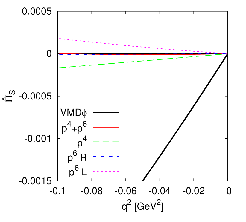
(a)

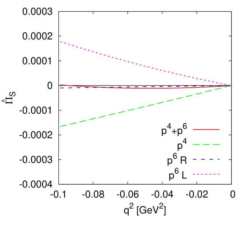
(b)

Figure 1: (a) The different contributions to $\hat{\Pi}_{S}(q^{2})$. The $p^{4}$ calculation, the pure two-loop part, $p^{6}R$, the $p^{6}$ part depending on the $p^{4}$ LECs, $p^{6}L$, and the pure LEC contribution as estimated in [29] using $\phi$-dominance, $VMD\phi$. (b) The different loop contributions only, i.e. the $VMD\phi$ contribution not included, with the same vertical scale as used in Fig. 2 but with a different range.

There is a large cancellation between the $p^{4}$ and $p^{6}$ contributions and the final result is very much dominated by the pure LEC contribution as estimated by $\phi$-exchange. In Fig. 1(b) we show the loop contributions with a smaller scale. For ease of comparison the vertical scale is the same as used in Fig. 2 but with a different range.

In Fig. 2 the loop contributions for the connected, (a), and disconnected, (b), parts are shown. It is clear that there is no simple ratio here as for the up-down case but in all cases the disconnected contribution is of opposite sign to the connected one and there are significant cancellations.

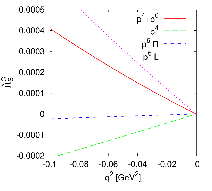
(a)

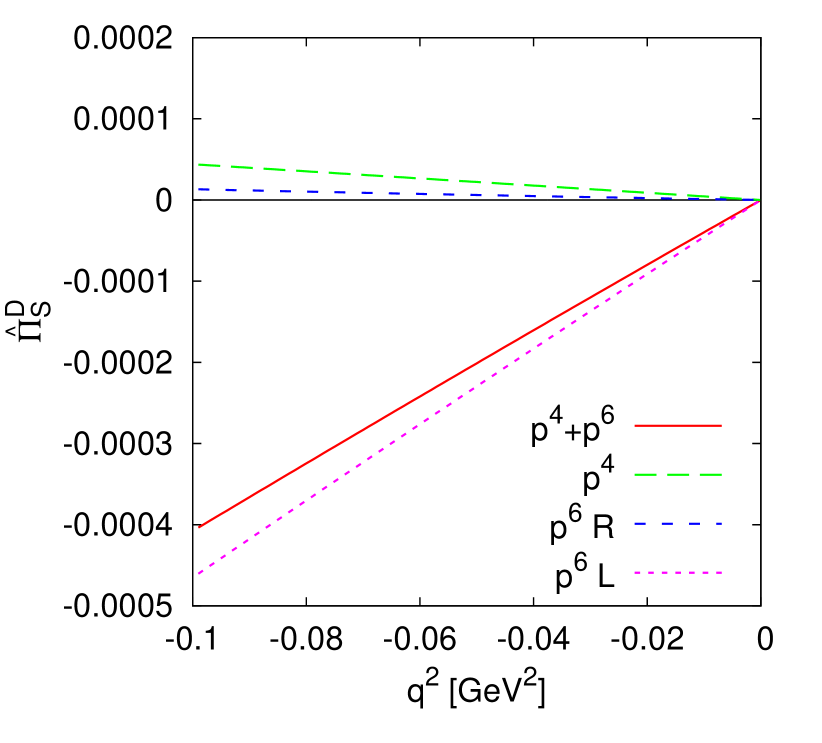
(b)

Figure 2: (a) The different contributions to the connected part, $\hat{\Pi}^{C}_{S}(q^{2})$. The $p^{4}$ calculation, the pure two-loop part, $p^{6}R$, and the $p^{6}$ part depending on the $p^{4}$ LECs, $p^{6}L$. The pure LEC contribution as estimated by $VMD\phi$ is not shown. (b) The different contributions to the disconnected part $\hat{\Pi}^{D}_{S}(q^{2})$. The $VMD\phi$ contribution is zero for this case.

The conclusion here is that the disconnected contribution is of order $-15\%$ of the total strange quark contribution with a sizable error. The error is both due to the large $p^{6}$ contribution and the uncertainty on the $VMD\phi$ estimate. The total strange quark contribution is by far dominated by the $VMD\phi$ part because even if individual loop contributions are of order $20\%$, there are large cancellations making the total strange quark contributions from the loops very small.

7 Numerical size of finite volume corrections

In this section we give numerical estimates of the finite volume effects for vector two-point functions and vacuum expectation values. In particular we address the questions of convergence of the finite volume corrections and the effects of using different twist angles for determining finite volume effects from lattice data. Note that we treat the time direction as infinite. The numerical input is the same as in section 6 except we have added

$$m_{\pi}L=4\,.$$ (44)

Our results are for the case with an infinite extent in the time direction. In realistic lattice calculations the time extent is often twice as large as the spatial directions and finite volume corrections fall approximately exponentially with the extent for values considered here. Our results are thus expected to be a reasonable approximation to the actually used lattice calculations. The programs we have used are for a general (Minkowski) time component of $q$ but below we only present numerical results for $q^{0}=0$.

7.1 Vector vacuum-expectation-value

As discussed in [15, 18], with twisted boundary conditions the vector currents can get a vacuum expectation value. The one loop result in standard ChPT was worked out in [18]. Here we add the two loop results as well as partial quenching and twisting. The formulas (36) and (B.3) are fully general but we present numerics here for the case where up and down masses are the same and sea and valence masses equal. To put the numbers in perspective we can compare with the results for the scalar vacuum expectation value. The finite volume corrections here are taken with zero twist using the results of [45]

$$\left<\bar{u}u\right>=\, -1.2~{}10^{-2}~{}\textrm{GeV}^{-3}, \left<\bar{u}u\right>^{V}(p^{4})=\, -2.4~{}10^{-5}~{}\textrm{GeV}^{-3},$$

$$\left<\bar{u}u\right>^{V}(p^{6}R)=\, 4.5~{}10^{-7}~{}\textrm{GeV}^{-3}, \left<\bar{u}u\right>^{V}(p^{6}L)=\, -1.2~{}10^{-7}~{}\textrm{GeV}^{-3}.$$ (45)

In Fig. 3(a) we plotted the result for $\left<\bar{u}\gamma^{\mu}u\right>$ for $\theta_{u}=(0,\theta,0,0)$ for the fully twisted case, i.e. both the sea and valence up quarks are twisted. In Fig. 3(b) we plot with the same twist angle but for the partially twisted case, only the up valence quark is twisted.

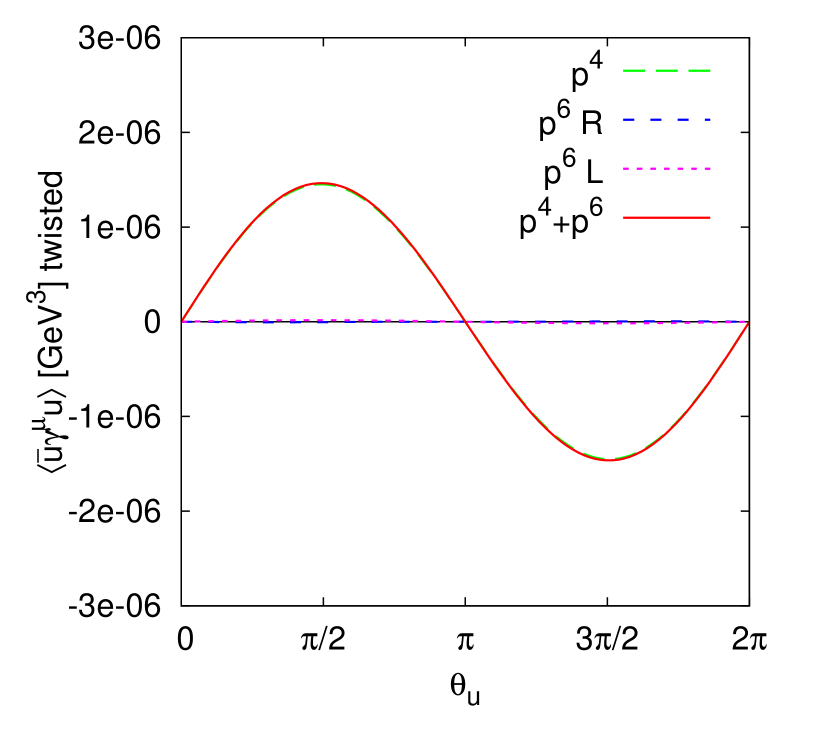
(a)

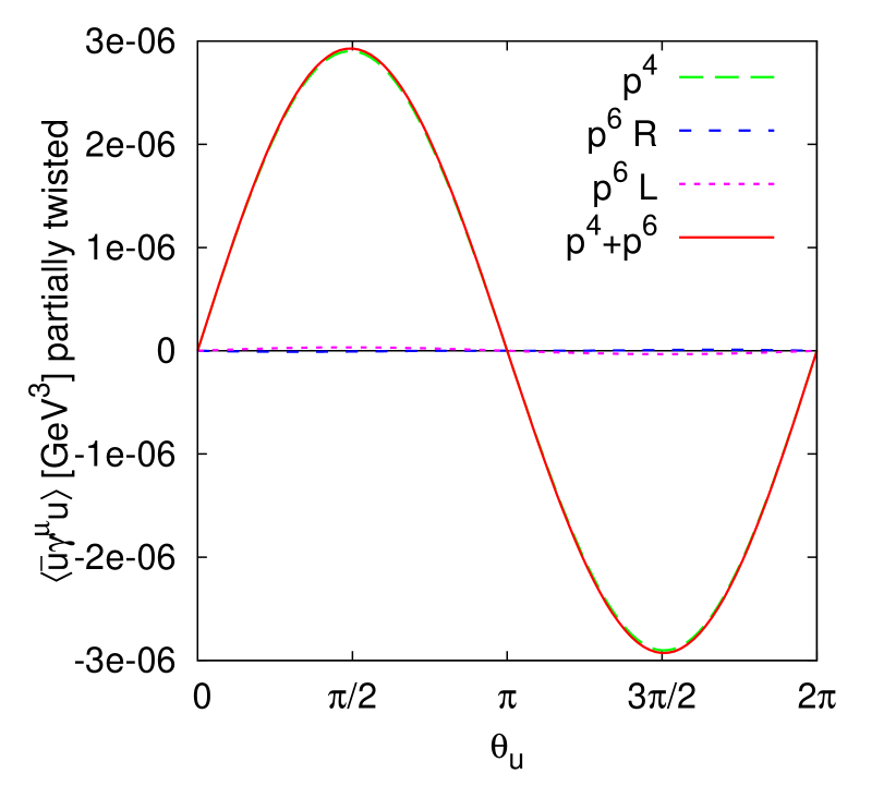
(b)

Figure 3: (a) The vacuum expectation value $\left<\bar{u}\gamma^{\mu}u\right>$ with the up valence and sea quark twisted with $\theta_{u}=(0,\theta,0,0)$. (b) Same but only the up valence quark twisted. In both cases the $x$-component or $\mu=1$ is plotted, the others vanish. The $p^{4}$ line is essentially indistinguishable from the $p^{4}+p^{6}$ line.

The finite volume corrections are roughly an order of magnitude smaller than for the scalar case in (7.1), but the same pattern is there. The $p^{6}$ corrections are very small. The partially twisted case is almost exactly a factor of two larger than the fully twisted case. The effects are strongly dominated by the pion loops and for these the difference at $p^{4}$ is exactly a factor of two. The vacuum expectation value $\left<\bar{d}\gamma^{\mu}d\right>$ with the up-quark fully twisted and no twist on the down quark is almost exactly minus $\left<\bar{u}\gamma^{\mu}u\right>$. Again it is exactly minus for the pion loops only. For the partially twisted up-quark $\left<\bar{d}\gamma^{\mu}d\right>$ vanishes since then no active quark has twist.

7.2 Finite volume corrections for the connected part

We now turn to the two-point functions. In the finite volume case we cannot simply present the combination $\hat{\Pi}(q^{2})$ since the subtraction at zero is not well defined, after all $\Pi^{\mu\nu}(q=0)\neq 0$. The relevant two-point function to use with twisted boundary conditions is the connected light part, $\Pi_{\pi^{+}}$. In the following we only twist the up-quark. We also put the up and down masses equal and sea and valence masses the same.

There is essentially no numerical difference between the fully twisted (both valence and sea up quark twisted) and partially twisted cases. We therefore present only the partially twisted case in the plots. The Ward identity is fulfilled in both cases but the right hand side of (18) gets the same numerical value in the fully twisted case from both the up and down vacuum expectation value, and in the partially twisted case only from the up vacuum expectation value.

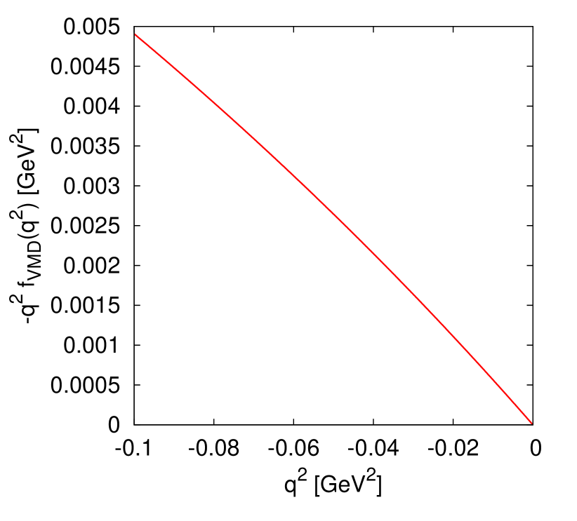
(a)

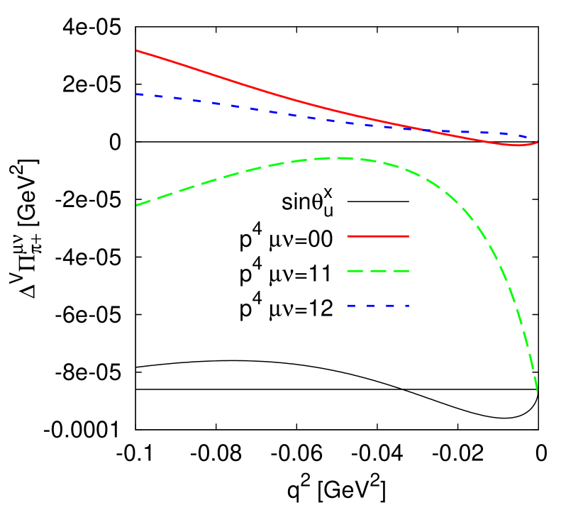
(b)

Figure 4: (a) $-q^{2}f_{\textrm{VMD}}(q^{2})$ as a function of $q^{2}$. This together with (47) and (48) can be used to judge the relative size of the finite volume effects in the following figures. (b) The finite volume corrections at $p^{4}$ for the spatially symmetric case. The lower straight line indicates zero around which $\sin\theta_{u}^{x}$ oscillates.

In order to show the size of the finite volume corrections we can compare with the naive VMD estimate. This corresponds to

$$\left.\Pi_{\pi^{+}}^{\mu\nu}\right|_{\mathrm{VMD}}=\left(q^{\mu}q^{\nu}-q^{2}g^{\mu\nu}\right)\frac{4F_{\pi}^{2}}{m_{V}^{2}-q^{2}}=\left(q^{\mu}q^{\nu}-q^{2}g^{\mu\nu}\right)f_{\textrm{VMD}}(q^{2}),$$ (46)

with $m_{V}=770$ MeV. When we choose $q=(0,\sqrt{-q^{2}},0,0)$ we have

$$\Pi^{00}=-\Pi^{22}=-\Pi^{33}=-q^{2}f_{\textrm{VMD}}(q^{2}),$$ (47)

and all others zero. Instead for $q=(0,\sqrt{-q^{2}/3},\sqrt{-q^{2}/3},\sqrt{-q^{2}/3})$ we have that

$$\Pi^{00}=\, -q^{2}f_{\textrm{VMD}}(q^{2}), \Pi^{ii}=\, \frac{2}{3}q^{2}f_{\textrm{VMD}}(q^{2}), \left.\Pi^{ij}\right|_{i\neq j}=\, -\frac{1}{3}q^{2}f_{\textrm{VMD}}(q^{2}),$$ (48)

with the others zero. We have plotted $-q^{2}f_{\textrm{VMD}}(q^{2})$ in Fig. 4(a).

We can now present the finite volume corrections. First we take the spatially symmetric twisted case. Here we use $\theta_{u}=q/L$ with $q=(0,\sqrt{q^{2}/3},\sqrt{q^{2}/3},\sqrt{q^{2}/3})$. The $p^{4}$ corrections are shown in Fig. 4(b). $\Pi^{\mu\nu}(q=0)\neq 0$ is clearly visible. The relative size of the correction compared to the VMD estimate is in the few % range (except of course at $q^{2}=0$ where it becomes infinite). Note that here we have $\Pi^{11}=\Pi^{22}=\Pi^{33}$, $\Pi^{01}=\Pi^{02}=\Pi^{03}=0$ and $\Pi^{12}=\Pi^{13}=\Pi^{23}$. In [27] they found that lowest order ChPT gives a good description of finite volume effects already at leading order ($p^{4}$). If this is the case, then the higher order corrections should turn out to be small, in contrast to the infinite volume case where they can be significant, see [29]. In Fig. 5

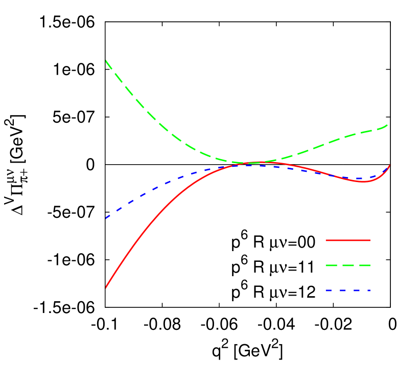
(a)

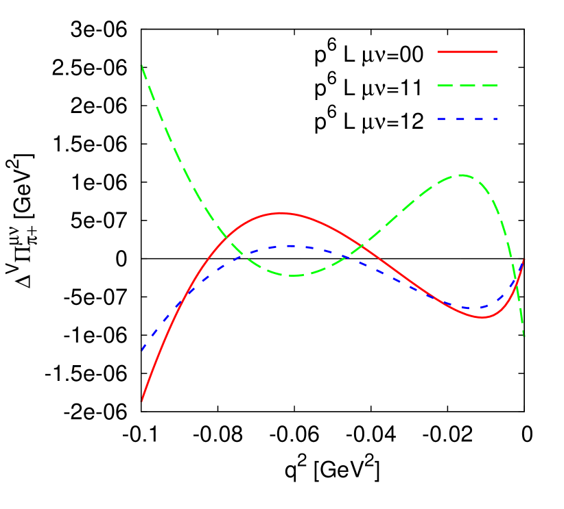
(b)

Figure 5: The parts of the finite volume corrections at $p^{6}$ for the spatially symmetric case(a) $p^{6}R$ (b) $p^{6}L$.

we plot the two parts of the finite volume correction for $\Pi_{\pi^{+}}$ at order $p^{6}$. We find that the correction is small, supporting the conclusion of [27]. The bottom curves in Fig. 4(b) and 6 show $\sin(\theta_{u}^{x})$ allowing to judge the type of twisting effects expected.

In Fig. 6(a) we show the full ($p^{4}+p^{6}$) finite volume correction for the spatially symmetric case. The $p^{4}$ result is included with thin dashed lines for comparison.

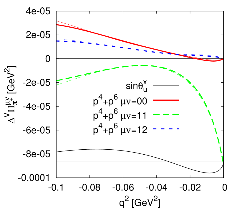
(a)

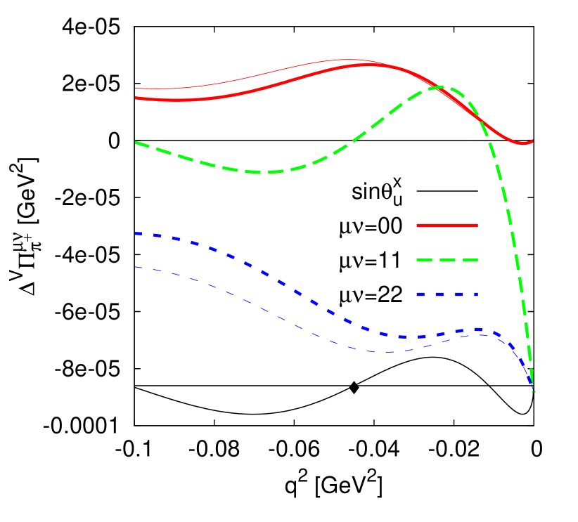
(b)

Figure 6: The finite volume corrections adding $p^{4}$ and $p^{6}$. The $p^{4}$ corrections are shown as the thin lines where each thin line should be associated with the same pattern and colour (and closest) thick line. The lower straight line indicates zero around which $\sin\theta_{u}^{x}$ oscillates. (a) The spatially symmetric case (b) Twisting only the $x$-direction. The diamond indicates a $q^{2}$ accessible with periodic boundary conditions.

Using the same twist angle in all spatial directions is common in lattice calculations of the HVP. It gives the possibility to average over several directions reducing the statistical error. However, the finite volume corrections do depend on how the twisting is done. We could have chosen to twist only in the $x$-direction. In that case we have $\theta_{u}=q/L$ with $q=(0,\sqrt{q^{2}},0,0)$ and $\Pi^{22}=\Pi^{33}$ and all elements with $\mu\neq\nu$ vanish. The full ($p^{4}+p^{6}$) finite volume corrections for this case are shown in Fig. 6(b). Again, the $p^{4}$ results are included with thin dashed lines.

Comparing the two halves of Fig. 6 we see quite different finite volume corrections. This can be used to test the size of the finite volume corrections using only lattice data by using two different ways of twisting that should reduce to the same $q^{2}$. This would also constitute a test of our predictions for the finite volume corrections. The quantity we will use for this is the average of the spatial diagonal components

$$\overline{\Pi}=\frac{1}{3}\sum_{i=1,2,3}\Pi^{ii}\,.$$ (49)

The finite volume corrections to $\overline{\Pi}$ are shown in Fig. 7. In (a) we show the $p^{4}$ result and in (b) the sum of the $p^{4}$ and $p^{6}$ results. There is a good convergence and the

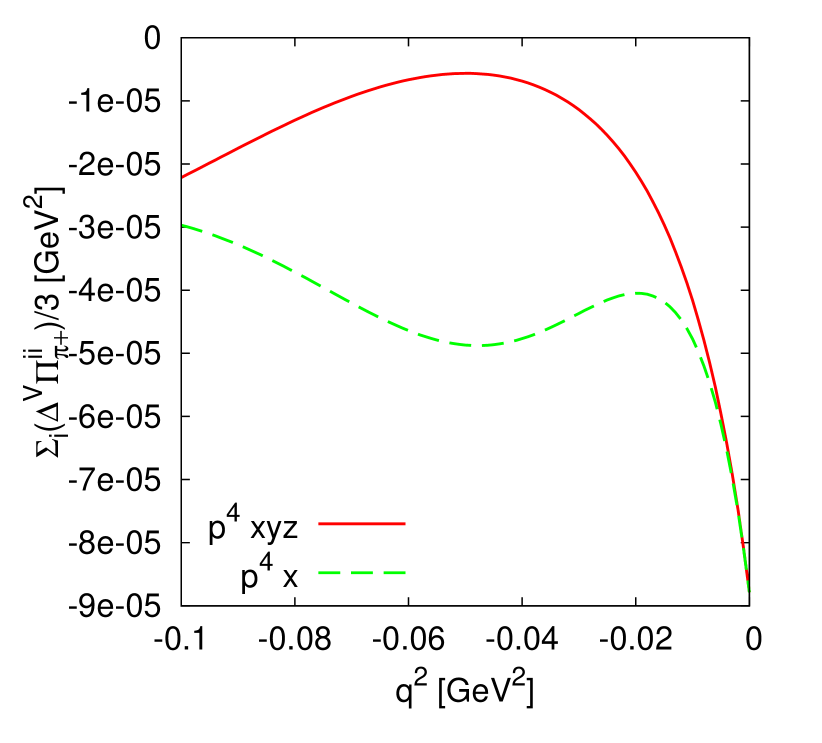
(a)

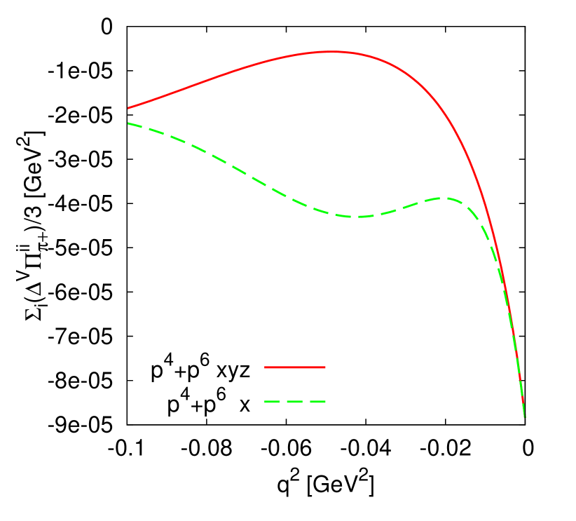
(b)

Figure 7: The finite volume corrections to the spatial average as defined in (49). $xyz$ is the spatially symmetric twisting and $x$ twisting only in the $x$-direction. (a) $p^{4}$ (b) Sum of $p^{4}$ and $p^{6}$.

difference between spatially symmetric twisting and twisting only in the $x$-direction is of similar size as the actual correction over a sizable range of $q^{2}$. This difference can thus be used to test the finite volume corrections using the same underlying set of configurations without having to resort to tricks like reweighting [46]. That the curves for the two cases coincide for $q^{2}=0$ is clear since then the twists vanish fully for both cases.

7.3 Finite volume corrections for the neutral case and disconnected part

In the previous subsection we could use (partial-)twisting to obtain any value of $q^{2}$ even at finite volume. For the neutral current where the twist on the quark and anti-quark cancel this is no longer true.

For $m_{\pi}L=4$, we only have access to $q^{2}=0,-0.045,-0.09$ GeV² for $|q^{2}|<0.1$ GeV². The values for q are respectively $q=(0,0,0,0)$, $q=(2\pi/L)(0,1,0,0)$ and $q=(2\pi/L)(0,1,1,0)$ (and permutations of $x,y,z$ and changes in signs of components).

The finite volume corrections are dominated by the lightest particle, the pion, and corrections due to kaons and eta are expected to be small. Our numerical results confirm this. Finite volume corrections require the presence of at least one loop in the contributions in ChPT, otherwise there is no propagating particle to feel the effect of the boundaries. Putting these two things together, the finite volume corrections are expected to show the relations between disconnected and connected parts of $\widetilde{\Pi}^{\mu\nu}$ in [29] and Sect. 5 for the three-flavour case exactly and the relations for the two-flavour case to a very good precision. This is indeed the case for our results. We thus only quote results for the connected contribution. The disconnected is $-1/2$ this and the sum of the two $+1/2$ the quoted numbers within the precision shown in Tab. 1.

The Ward identity $q_{\mu}\Pi^{\mu\nu}=0$ is also satisfied, relating a number of the nonzero-components. This together with the symmetries determines the nonzero components not listed. The relations are given in the last column in Tab. 1. The size of the corrections should be compared with the results in Fig. 4(a) as discussed in the previous subsection. The value at $q=(0,0,0,0)$ agrees of course with those shown in the figures for the connected contribution. The size of the corrections is similar to the case with twist discussed earlier.

$q/(2\pi/L)$		$\Pi^{00}_{U}$	$\Pi^{11}_{U}$	$\Pi^{33}_{U}$
		$[10^{-5}~{}$GeV${}^{2}]$	$[10^{-5}~{}$GeV${}^{2}]$	$[10^{-5}~{}$GeV${}^{2}]$
(0,0,0,0)	$p^{4}$	$-$0.000	$-$8.785	$-$8.785	$\Pi^{22}_{U}=\Pi^{33}_{U}$
	$p^{6}~{}R$	$-$0.000	$-$0.045	$-$0.045
	$p^{6}~{}L$	$-$0.000	$-$0.102	$-$0.102
	sum	$-$0.000	$-$8.842	$-$8.842
(0,1,0,0)	$p^{4}$	$-$2.840	$-$0.000	$-$7.294	$\Pi^{22}_{U}=\Pi^{33}_{U}$
	$p^{6}~{}R$	$-$0.091	$-$0.000	$-$0.223
	$p^{6}~{}L$	$-$0.117	$-$0.000	$-$0.633
	sum	$-$2.632	$-$0.000	$-$6.438
(0,1,1,0)	$p^{4}$	$-$3.604	$-$2.415	$-$6.442	$\Pi^{22}_{U}=\Pi^{11}_{U}$
	$p^{6}~{}R$	$-$0.195	$-$0.128	$-$0.338	$\Pi^{12}_{U}=-\Pi^{11}_{U}$
	$p^{6}~{}L$	$-$0.458	$-$0.376	$-$1.144	$\Pi^{21}_{U}=-\Pi^{11}_{U}$
	sum	$-$2.951	$-$1.911	$-$4.960

Table 1: The finite volume corrections to the components of $\Pi^{\mu\nu}_{U}$ for the connected part for low lying momenta available with periodic boundary conditions. The disconnected part is essentially $-1/2$ the connected part as discussed in the text. The last columns indicate components which are related to the explicitly presented ones. Components not mentioned are zero.

The use of different twists with the same $q^{2}$ has been discussed above as a possible way to test the finite volume corrections without having to generate a lattice with a different volume. The same can be done here. Partial twisting does not allow for different values of $q^{2}$ but it does give different finite volume corrections since the charged mesons in the loops will be affected. As an example we have looked at the values for $q=(0,0,0,0)$ but twisting the valence up-quark with a twist angle $\theta=(0,\pi/2,\pi/2,\pi/2)$. Now the relation between the disconnected and connected part of about $-1/2$ is no longer valid and our numerics also show this. The results for the connected and disconnected parts are shown in Tab. 2. Given the symmetries of the input we have here that $\Pi^{00}_{U}=\Pi^{0i}_{U}=0$, the spatial diagonal elements are all the same and the spatial off-diagonal elements are also all the same. The disconnected part has only small changes compared to the case with no twist but the connected part changes considerably. So again, using different twists can be used to check the finite volume corrections.

	$\Pi^{11}_{U}$	$\Pi^{12}_{U}$	$\Pi^{11}_{U}$	$\Pi^{12}_{U}$
	$[10^{-5}~{}$GeV${}^{2}]$	$[10^{-5}~{}$GeV${}^{2}]$	$[10^{-5}~{}$GeV${}^{2}]$	$[10^{-5}~{}$GeV${}^{2}]$
	Connected		Disconnected
$p^{4}$	$-$0.065	$-$0.915	$-$4.392	0.000
$p^{6}~{}R$	$-$0.012	$-$0.002	$-$0.011	0.003
$p^{6}~{}L$	$-$0.001	$-$0.014	$-$0.051	0.000
sum	$-$0.054	$-$0.926	$-$4.432	0.003

Table 2: The finite volume corrections to the components of $\Pi^{\mu\nu}_{U}$ for the connected and disconnected part with $q=(0,0,0,0)$ and a partially twisted up quark with twist angle $\theta=(0,\pi/2,\pi/2,\pi/2)$. Note the difference with Table 1.

8 Conclusion

In this paper we have calculated the vector one-point and two-point functions at $p^{4}$ and $p^{6}$ using PQChPT in finite volume with twisted boundary conditions. We have calculated one connected and one disconnected two-point function. In PQChPT this is all that is needed to obtain all vector two-point functions. The connected two-point function was calculated by considering a flavor charged current with equal masses. The disconnected two-point function was calculated using two neutral currents with different flavors.

Extending the work of [13] and our work in [29] we have used the PQ expressions to give a numerical estimate of the ratio of disconnected to connected contributions for the strange quark part of the electromagnetic current. Using VMD for the $\phi$ meson to estimate the pure LEC contribution we obtain a ratio of about $-15\%$.

We have also looked at the effects from finite volume and twisted boundary conditions. The $p^{6}$ contributions to the finite volume corrections are small when compared with the $p^{4}$ contributions which supports the conclusion of [27] that $p^{4}$ describes the observed finite volume effects. We also point out that the difference between estimates using different twist angles at the same $q^{2}$ can be used to estimate the finite volume corrections using a single lattice volume.

Appendix A Integral notation

The loop integrals needed when calculating vector two-point functions are

$$A^{\{\,,\mu,\mu\nu\}}\left([m^{2}]^{n}\right)=\, \frac{1}{i}\int_{V}\frac{d^{d}k}{(2\pi)^{d}}\frac{\{1,k^{\mu},k^{\mu}k^{\nu}\}}{(k^{2}-m^{2})^{n}}\,,$$

$$B^{\{\,,\mu,\mu\nu,\mu\nu\alpha\}}\left([m_{1}^{2}]^{n_{1}},[m_{2}^{2}]^{n_{2}},q\right)=\, \frac{1}{i}\int_{V}\frac{d^{d}k}{(2\pi)^{d}}\frac{\{1,k^{\mu},k^{\mu}k^{\nu},k^{\mu}k^{\nu}k^{\alpha}\}}{(k^{2}-m_{1}^{2})^{n_{1}}((q-k)^{2}-m_{2}^{2})^{n_{2}}}\,.$$ (50)

When twisted boundary conditions are used the allowed momenta $k$ in $k^{2}-m^{2}$ are indicated by the mass, e.g. allowed momenta in $k^{2}-m_{\pi^{+}}^{2}$ are the $\pi^{+}$ momenta, see [18]. Note that the definitions of the integrals include poles of any order. For poles of order one we use notation where we skip the square brackets and order of the pole, i.e. $A([m^{2}]^{1})\equiv A(m^{2})$.

The integrals above contain both the finite volume and infinite volume contributions. Examplifying with $A$ and suppressing all arguments, we split the integrals according to

$$A=\, \frac{C_{A}}{\bar{\epsilon}}+A^{\mathcal{V}}+\epsilon A^{\epsilon}+\mathcal{O}(\epsilon^{2}),$$

$$\frac{1}{\bar{\epsilon}}=\, \frac{1}{\epsilon}+\ln(4\pi)+1-\gamma.$$ (51)

The constant $C_{A}$ is the residue of the $1/\bar{\epsilon}$ pole and differs from integral to integral. We renormalize our expressions using the ChPT version of $\overline{MS}$ where parts proportional to $1/\bar{\epsilon}$ cancel. $A^{\mathcal{V}}$ then contains the part of the infinite volume integral which remains after renormalization plus the finite volume correction. We express this as

$$A^{\mathcal{V}}=\bar{A}+A^{V},$$ (52)

where $\bar{A}$ is the infinite volume part and $A^{V}$ is the finite volume correction.

The infinite volume part of the integrals, including the residues of the poles, can be found from [48] using that the higher pole integrals can be obtained by derivatives with respect to the masses. Methods for evaluating the finite volume correction, as well as expressions for some of the integrals, can be found in [43, 49, 18]. In [18] we gave explicit expressions, in terms of Jacobi theta functions, for the finite volume corrections to all of the integrals except for $B^{\mu\nu\alpha}\left([m_{1}^{2}]^{n_{1}},[m_{2}^{2}]^{n_{2}},q\right)$. The expression for the finite volume correction to $B^{\mu\nu\alpha}\left([m_{1}^{2}]^{n_{1}},[m_{2}^{2}]^{n_{2}},q\right)$ is

$$B^{V\mu\nu\alpha} \left([m_{1}^{2}]^{n_{1}},[m_{2}^{2}]^{n_{2}},q\right)=\frac{\Gamma(n_{1}+n_{2})}{\Gamma(n_{1})\Gamma(n_{2})}\int dx(1-x)^{n_{1}-1}x^{n_{2}-1}\times\Big{(}$$

$$A^{V\mu\nu\alpha}([\tilde{m}^{2}]^{n_{1}+n_{2}})+x(\delta_{\rho}^{\mu}\delta_{\sigma}^{\nu}q^{\alpha}+\delta_{\rho}^{\mu}q^{\nu}\delta_{\sigma}^{\alpha}+q^{\mu}\delta_{\rho}^{\nu}\delta_{\sigma}^{\mu})A^{V\rho\sigma}([\tilde{m}^{2}]^{n_{1}+n_{2}})$$

$$+ x^{2}(\delta_{\rho}^{\mu}q^{\nu}q^{\alpha}+q^{\mu}\delta_{\rho}^{\nu}q^{\alpha}+q^{\mu}q^{\nu}\delta_{\rho}^{\alpha})A^{V\rho}([\tilde{m}^{2}]^{n_{1}+n_{2}})+x^{3}q^{\mu}q^{\nu}q^{\alpha}A^{V}([\tilde{m}^{2}]^{n_{1}+n_{2}})\Big{)}\,,$$ (53)

where

$$\tilde{m}^{2}=(1-x)m_{1}^{2}+xm_{2}^{2}-x(1-x)q^{2},$$ (54)

and the integrals on the right hand side should be evaluated with the twist angle

$$\vec{\tilde{\theta}}=\vec{\theta}-x\vec{q}L.$$ (55)

In the actual results we have split the integrals as

$$B^{\mu\nu\alpha} =q^{\mu}q^{\nu}q^{\alpha}B_{31}+(g^{\mu\nu}q^{\alpha}+g^{\mu\alpha}q^{\nu}+g^{\nu\alpha}q^{\mu})B_{32}+B_{33}^{\mu\nu\alpha},$$

$$B^{\mu\nu} =q^{\mu}q^{\nu}B_{21}+g^{\mu\nu}B_{22}+B_{23}^{\mu\nu},$$

$$B^{\mu} =q^{\mu}B_{1}+B_{2}^{\mu},$$

$$A^{\mu\nu} =g^{\mu\nu}A_{22}+A_{23}^{\mu\nu},$$ (56)

where all arguments are suppressed.

The diagonal integral introduced in (3) can in principle be split up using the residue notation of [42] so that all integrals are of the form (A). This corresponds to partial fractioning $\mathcal{D}_{ab}$. This leads to longer and more difficult to read expressions and we keep the diagonal propagator intact using notation such as

$$A(\mathcal{D}_{ab})=\frac{1}{i}\int_{V}\frac{d^{d}k}{(2\pi)^{d}}\left(-\frac{1}{3}\frac{(p^{2}-m_{1}^{2})(p^{2}-m_{2}^{2})(p^{2}-m_{3}^{2})}{(p^{2}-m_{a}^{2})(p^{2}-m_{b}^{2})(p^{2}-m_{\pi^{0}}^{2})(p^{2}-m_{\eta}^{2})}\right).$$ (57)

The residue notation is used in the numerical implementation of our results.

Appendix B Analytical results

In this appendix we present the analytical expressions for vector two-point functions and one-point functions at $p^{6}$ in PQChPT in finite volume. In the case of $\Pi_{\pi^{+}_{v}}$ the expressions also contain effects from partially twisted boundary conditions. Additionally the expressions contain both the infinite volume part and the finite volume correction, see section 4, where the $p^{4}$ expressions are presented. Note that all expressions are given using lowest order masses. All expressions given will be implemented numerically in CHIRON [31, 32].

B.1 $\Pi_{\pi^{+}_{v}}^{\mathcal{V}\mu\nu}$ at $p^{6}$

The results presented below are for the various components of $\Pi_{\pi^{+}_{v}}^{\mathcal{V}(6)}$. These are the infinite and finite volume $p^{6}$ expressions for $\Pi_{\pi^{+}_{v}}$. The results are the partially twisted ones. Note, however, that the expressions are for the case when the two valence quark masses are set equal. The case where the valence quark masses differ is much longer and will not be given here.

$$F_{0}^{2} \Pi_{0\pi^{+}_{v}}^{\mathcal{V}(6)}=$$

$$+A^{\mathcal{V}}(m_{x\mathcal{S}}^{2})\Big{(}-4L^{10}_{r}-4L^{9}_{r}-\frac{1}{2}B^{\mathcal{V}}(m_{x\mathcal{S}^{\prime}}^{2},m_{\mathcal{S}^{\prime}y}^{2},q)+B_{1}^{\mathcal{V}}(m_{x\mathcal{S}^{\prime}}^{2},m_{\mathcal{S}^{\prime}y}^{2},q)\Big{)}$$

$$+A^{\mathcal{V}}(m_{y\mathcal{S}}^{2})\Big{(}-4L^{10}_{r}+4L^{9}_{r}+4B_{21}^{\mathcal{V}}(m_{x\mathcal{S}^{\prime}}^{2},m_{\mathcal{S}^{\prime}y}^{2},q)+\frac{7}{6}B^{\mathcal{V}}(m_{x\mathcal{S}^{\prime}}^{2},m_{\mathcal{S}^{\prime}y}^{2},q)$$

$$\hskip 28.45274pt-\frac{13}{3}B_{1}^{\mathcal{V}}(m_{x\mathcal{S}^{\prime}}^{2},m_{\mathcal{S}^{\prime}y}^{2},q)\Big{)}$$

$$+\Big{(}A^{\mathcal{V}}(m_{xy}^{2})-A^{\mathcal{V}}(m_{xx}^{2})\Big{)}\Big{(}-8B_{21}^{\mathcal{V}}([m_{xx}^{2}]^{2},m_{xy}^{2},q)m_{xx}^{2}+\frac{8}{3}B^{\mathcal{V}}(m_{xy}^{2},m_{xx}^{2},q)$$

$$\hskip 28.45274pt-2B^{\mathcal{V}}([m_{xx}^{2}]^{2},m_{xy}^{2},q)m_{xx}^{2}-\frac{16}{3}B_{1}^{\mathcal{V}}(m_{xy}^{2},m_{xx}^{2},q)+8B_{1}^{\mathcal{V}}([m_{xx}^{2}]^{2},m_{xy}^{2},q)m_{xx}^{2}\Big{)}$$

$$+A^{\mathcal{V}}(\mathcal{D}_{x\mathcal{S}})\Big{(}+4B_{21}^{\mathcal{V}}([m_{x\mathcal{S}}^{2}]^{2},m_{\mathcal{S}y}^{2},q)m_{x\mathcal{S}}^{2}+4B_{21}^{\mathcal{V}}([m_{\mathcal{S}y}^{2}]^{2},m_{x\mathcal{S}}^{2},q)m_{x\mathcal{S}}^{2}$$

$$\hskip 28.45274pt+B^{\mathcal{V}}([m_{x\mathcal{S}}^{2}]^{2},m_{\mathcal{S}y}^{2},q)m_{x\mathcal{S}}^{2}+B^{\mathcal{V}}([m_{\mathcal{S}y}^{2}]^{2},m_{x\mathcal{S}}^{2},q)m_{x\mathcal{S}}^{2}-4B_{1}^{\mathcal{V}}([m_{x\mathcal{S}}^{2}]^{2},m_{\mathcal{S}y}^{2},q)m_{x\mathcal{S}}^{2}$$

$$\hskip 28.45274pt-4B_{1}^{\mathcal{V}}([m_{\mathcal{S}y}^{2}]^{2},m_{x\mathcal{S}}^{2},q)m_{x\mathcal{S}}^{2}\Big{)}$$

$$+A^{\mathcal{V}\rho}(m_{x\mathcal{S}}^{2})\Big{(}-4B_{31}^{\mathcal{V}}([m_{x\mathcal{S}^{\prime}}^{2}]^{2},m_{\mathcal{S}^{\prime}y}^{2},q)q_{\rho}+4B_{21}^{\mathcal{V}}([m_{x\mathcal{S}^{\prime}}^{2}]^{2},m_{\mathcal{S}^{\prime}y}^{2},q)q_{\rho}$$

$$\hskip 28.45274pt-B_{1}^{\mathcal{V}}([m_{x\mathcal{S}^{\prime}}^{2}]^{2},m_{\mathcal{S}^{\prime}y}^{2},q)q_{\rho}-B_{2\rho}^{\mathcal{V}}([m_{x\mathcal{S}^{\prime}}^{2}]^{2},m_{\mathcal{S}^{\prime}y}^{2},q)\Big{)}$$

$$+A^{\mathcal{V}\rho}(m_{y\mathcal{S}}^{2})\Big{(}+4B_{31}^{\mathcal{V}}([m_{\mathcal{S}^{\prime}y}^{2}]^{2},m_{x\mathcal{S}^{\prime}}^{2},q)q_{\rho}-4B_{21}^{\mathcal{V}}([m_{\mathcal{S}^{\prime}y}^{2}]^{2},m_{x\mathcal{S}^{\prime}}^{2},q)q_{\rho}$$

$$\hskip 28.45274pt+B_{1}^{\mathcal{V}}([m_{\mathcal{S}^{\prime}y}^{2}]^{2},m_{x\mathcal{S}^{\prime}}^{2},q)q_{\rho}+B_{2\rho}^{\mathcal{V}}([m_{\mathcal{S}^{\prime}y}^{2}]^{2},m_{x\mathcal{S}^{\prime}}^{2},q)\Big{)}$$

$$-A^{\mathcal{V}\rho}(m_{\mathcal{S}^{\prime}\mathcal{S}}^{2})\Big{(}+4B_{31}^{\mathcal{V}}([m_{x\mathcal{S}}^{2}]^{2},m_{\mathcal{S}y}^{2},q)q_{\rho}-4B_{31}^{\mathcal{V}}([m_{\mathcal{S}y}^{2}]^{2},m_{x\mathcal{S}}^{2},q)q_{\rho}$$

$$\hskip 28.45274pt+4B_{21}^{\mathcal{V}}([m_{x\mathcal{S}}^{2}]^{2},m_{\mathcal{S}y}^{2},q)q_{\rho}-4B_{21}^{\mathcal{V}}([m_{\mathcal{S}y}^{2}]^{2},m_{x\mathcal{S}}^{2},q)q_{\rho}+B_{1}^{\mathcal{V}}([m_{x\mathcal{S}}^{2}]^{2},m_{\mathcal{S}y}^{2},q)q_{\rho}$$

$$\hskip 28.45274pt-B_{1}^{\mathcal{V}}([m_{\mathcal{S}y}^{2}]^{2},m_{x\mathcal{S}}^{2},q)q_{\rho}+B_{2\rho}^{\mathcal{V}}([m_{x\mathcal{S}}^{2}]^{2},m_{\mathcal{S}y}^{2},q)-B_{2\rho}^{\mathcal{V}}([m_{\mathcal{S}y}^{2}]^{2},m_{x\mathcal{S}}^{2},q)\Big{)}$$

$$+q^{2}B^{\mathcal{V}}(m_{x\mathcal{S}}^{2},m_{\mathcal{S}y}^{2},q)\Big{(}+2B_{21}^{\mathcal{V}}(m_{x\mathcal{S}^{\prime}}^{2},m_{\mathcal{S}^{\prime}y}^{2},q)-B_{1}^{\mathcal{V}}(m_{x\mathcal{S}^{\prime}}^{2},m_{\mathcal{S}^{\prime}y}^{2},q)+\frac{1}{2}B^{\mathcal{V}}(m_{x\mathcal{S}^{\prime}}^{2},m_{\mathcal{S}^{\prime}y}^{2},q)$$

$$\hskip 28.45274pt+4L^{9}_{r}\Big{)}$$

$$+\Big{(}B^{\mathcal{V}}([m_{x\mathcal{S}}^{2}]^{2},m_{\mathcal{S}y}^{2},q)+B^{\mathcal{V}}([m_{y\mathcal{S}}^{2}]^{2},m_{x\mathcal{S}}^{2},q)\Big{)}\Big{(}+8m_{x\mathcal{S}}^{4}\Big{(}2L^{8}_{r}-L^{5}_{r}\Big{)}$$

$$\hskip 28.45274pt+8m_{\mathcal{S}^{\prime}\mathcal{S}^{\prime}}^{2}m_{x\mathcal{S}}^{2}\Big{(}2L^{6}_{r}-L^{4}_{r}\Big{)}\Big{)}$$

$$-\frac{4}{3}B^{\mathcal{V}}(m_{x\mathcal{S}^{\prime}}^{2},m_{\mathcal{S}^{\prime}y}^{2},q)\Big{(}+B_{21}^{\mathcal{V}}(m_{x\mathcal{S}}^{2},m_{\mathcal{S}y}^{2},q)q^{2}+B_{22}^{\mathcal{V}}(m_{x\mathcal{S}}^{2},m_{\mathcal{S}y}^{2},q)+B_{1}^{\mathcal{V}}(m_{x\mathcal{S}}^{2},m_{\mathcal{S}y}^{2},q)q^{2}\Big{)}$$

$$+B^{\mathcal{V}}(m_{xy}^{2},m_{xx}^{2},q)^{2}\Big{(}-\frac{5}{3}q^{2}+2m_{xx}^{2}\Big{)}$$

$$+B^{\mathcal{V}}(m_{xy}^{2},m_{xx}^{2},q)\Big{(}+\frac{20}{3}B_{1}^{\mathcal{V}}(m_{xy}^{2},m_{xx}^{2},q)q^{2}-8B_{1}^{\mathcal{V}}(m_{xy}^{2},m_{xx}^{2},q)m_{xx}^{2}\Big{)}$$

$$+q^{2}B_{1}^{\mathcal{V}}(m_{x\mathcal{S}}^{2},m_{\mathcal{S}y}^{2},q)\Big{(}-2B_{21}^{\mathcal{V}}(m_{x\mathcal{S}^{\prime}}^{2},m_{\mathcal{S}^{\prime}y}^{2},q)+\frac{5}{3}B_{1}^{\mathcal{V}}(m_{x\mathcal{S}^{\prime}}^{2},m_{\mathcal{S}^{\prime}y}^{2},q)-8L^{9}_{r}\Big{)}$$

$$-\Big{(}B_{1}^{\mathcal{V}}([m_{x\mathcal{S}}^{2}]^{2},m_{\mathcal{S}y}^{2},q)+B_{1}^{\mathcal{V}}([m_{y\mathcal{S}}^{2}]^{2},m_{x\mathcal{S}}^{2},q)\Big{)}\Big{(}+32m_{x\mathcal{S}}^{4}\Big{(}2L^{8}_{r}-L^{5}_{r}\Big{)}$$

$$\hskip 28.45274pt+32m_{\mathcal{S}^{\prime}\mathcal{S}^{\prime}}^{2}m_{x\mathcal{S}}^{2}\Big{(}2L^{6}_{r}-L^{4}_{r}\Big{)}\Big{)}$$

$$+B_{1}^{\mathcal{V}}(m_{x\mathcal{S}^{\prime}}^{2},m_{\mathcal{S}^{\prime}y}^{2},q)\Big{(}+\frac{14}{3}B_{21}^{\mathcal{V}}(m_{x\mathcal{S}}^{2},m_{\mathcal{S}y}^{2},q)q^{2}+\frac{20}{3}B_{22}^{\mathcal{V}}(m_{x\mathcal{S}}^{2},m_{\mathcal{S}y}^{2},q)\Big{)}$$

$$+B_{1}^{\mathcal{V}}(m_{xy}^{2},m_{xx}^{2},q)^{2}\Big{(}-\frac{20}{3}q^{2}+8m_{xx}^{2}\Big{)}$$

$$-4B_{21}^{\mathcal{V}}(m_{x\mathcal{S}}^{2},m_{\mathcal{S}y}^{2},q)\Big{(}+q^{2}B_{21}^{\mathcal{V}}(m_{x\mathcal{S}^{\prime}}^{2},m_{\mathcal{S}^{\prime}y}^{2},q)+B_{22}^{\mathcal{V}}(m_{x\mathcal{S}^{\prime}}^{2},m_{\mathcal{S}^{\prime}y}^{2},q)\Big{)}$$

$$+\Big{(}B_{21}^{\mathcal{V}}([m_{x\mathcal{S}}^{2}]^{2},m_{\mathcal{S}y}^{2},q)+B_{21}^{\mathcal{V}}([m_{\mathcal{S}y}^{2}]^{2},m_{x\mathcal{S}}^{2},q)\Big{)}\Big{(}+32m_{x\mathcal{S}}^{4}\Big{(}2L^{8}_{r}-L^{5}_{r}\Big{)}$$

$$\hskip 28.45274pt+32m_{x\mathcal{S}}^{2}m_{\mathcal{S}^{\prime}\mathcal{S}^{\prime}}^{2}\Big{(}2L^{6}_{r}-L^{4}_{r}\Big{)}\Big{)}$$

$$-16B_{22}^{\mathcal{V}}(m_{x\mathcal{S}}^{2},m_{\mathcal{S}y}^{2},q)L^{9}_{r}-B_{2}^{\mathcal{V}\alpha}(m_{x\mathcal{S}}^{2},m_{\mathcal{S}y}^{2},q)B_{2\alpha}^{\mathcal{V}}(m_{x\mathcal{S}^{\prime}}^{2},m_{\mathcal{S}^{\prime}y}^{2},q).$$ (58)

$$F_{0}^{2} \Pi_{1\pi^{+}_{v}}^{\mathcal{V}(6)}=$$

$$\Big{(}A^{\mathcal{V}}(m^{2}_{xy})-A^{\mathcal{V}}(m^{2}_{xx})\Big{)}\Big{(}8m^{2}_{xx}B_{22}^{\mathcal{V}}([m^{2}_{xx}]^{2},m^{2}_{xy},q)-2m^{2}_{xx}A^{\mathcal{V}}([m^{2}_{xx}]^{2})+A^{\mathcal{V}}(m^{2}_{xy})$$

$$\hskip 28.45274pt-A^{\mathcal{V}}(m^{2}_{xx})\Big{)}$$

$$-m^{2}_{\mathcal{S}x}\Big{(}4B_{22}^{\mathcal{V}}(m^{2}_{x\mathcal{S}},[m^{2}_{\mathcal{S}y}]^{2},q)+4B_{22}^{\mathcal{V}}([m^{2}_{x\mathcal{S}}]^{2},m^{2}_{\mathcal{S}y},q)-A^{\mathcal{V}}([m^{2}_{x\mathcal{S}}]^{2})-A^{\mathcal{V}}([m^{2}_{y\mathcal{S}}]^{2})\Big{)}$$

$$\hskip 28.45274pt\times(16m^{2}_{\mathcal{S}^{\prime}\mathcal{S}^{\prime}}L_{6}^{r}-8m^{2}_{\mathcal{S}^{\prime}\mathcal{S}^{\prime}}L_{4}^{r}+16m^{2}_{\mathcal{S}x}L_{8}^{r}-8m^{2}_{\mathcal{S}x}L_{5}^{r}+A^{\mathcal{V}}(\mathcal{D}_{x\mathcal{S}}))$$

$$-2\Big{(}A^{\mathcal{V}}(m^{2}_{x\mathcal{S}})+A^{\mathcal{V}}(m^{2}_{y\mathcal{S}})\Big{)}\Big{(}2L_{10}^{r}q^{2}+B_{22}^{\mathcal{V}}(m^{2}_{x\mathcal{S}^{\prime}},m^{2}_{\mathcal{S}^{\prime}y},q)\Big{)}$$

$$+q^{\beta}\Big{(}A_{\beta}^{\mathcal{V}}(m^{2}_{x\mathcal{S}})-A_{\beta}^{\mathcal{V}}(m^{2}_{\mathcal{S}^{\prime}\mathcal{S}})\Big{)}\Big{(}4B_{32}^{\mathcal{V}}([m^{2}_{x\mathcal{S}^{\prime}}]^{2},m^{2}_{\mathcal{S}^{\prime}y},q)\Big{)}$$

$$-q^{\beta}\Big{(}A_{\beta}^{\mathcal{V}}(m^{2}_{y\mathcal{S}})-A_{\beta}^{\mathcal{V}}(m^{2}_{\mathcal{S}^{\prime}\mathcal{S}})\Big{)}\Big{(}4B_{22}^{\mathcal{V}}(m^{2}_{x\mathcal{S}^{\prime}},[m^{2}_{\mathcal{S}^{\prime}y}]^{2},q)-4B_{32}^{\mathcal{V}}(m^{2}_{x\mathcal{S}^{\prime}},[m^{2}_{\mathcal{S}^{\prime}y}]^{2},q)\Big{)}$$

$$-2B_{22}^{\mathcal{V}}(m^{2}_{x\mathcal{S}},m^{2}_{\mathcal{S}y},q)\Big{(}8L_{9}^{r}q^{2}-2B_{22}^{\mathcal{V}}(m^{2}_{x\mathcal{S}^{\prime}},m^{2}_{\mathcal{S}^{\prime}y},q)\Big{)}+8L_{9}^{r}q^{\beta}\Big{(}A_{\beta}^{\mathcal{V}}(m^{2}_{x\mathcal{S}})-A_{\beta}^{\mathcal{V}}(m^{2}_{y\mathcal{S}})\Big{)}$$

$$+A^{\mathcal{V}}(m^{2}_{y\mathcal{S}})A^{\mathcal{V}}(m^{2}_{x\mathcal{S}^{\prime}})+A^{\mathcal{V}\beta}([m^{2}_{x\mathcal{S}^{\prime}}]^{2})\Big{(}A_{\beta}^{\mathcal{V}}(m^{2}_{\mathcal{S}^{\prime}\mathcal{S}})-A_{\beta}^{\mathcal{V}}(m^{2}_{x\mathcal{S}})\Big{)}$$

$$+A^{\mathcal{V}\beta}([m^{2}_{y\mathcal{S}^{\prime}}]^{2})\Big{(}A_{\beta}^{\mathcal{V}}(m^{2}_{\mathcal{S}^{\prime}\mathcal{S}})-A_{\beta}^{\mathcal{V}}(m^{2}_{y\mathcal{S}})\Big{)}.$$ (59)

$$F_{0}^{2} \Pi^{\mathcal{V}(6)\mu\nu}_{2\pi^{+}_{v}}=$$

$$+A^{\mathcal{V}\rho}(m_{x\mathcal{S}}^{2})\Big{(}+2B_{22}^{\mathcal{V}}([m_{x\mathcal{S}^{\prime}}^{2}]^{2},m_{\mathcal{S}^{\prime}y}^{2},q)\delta_{\rho}^{\nu}q^{\mu}-4B_{3}2^{\mathcal{V}}([m_{x\mathcal{S}^{\prime}}^{2}]^{2},m_{\mathcal{S}^{\prime}y}^{2},q)\delta_{\rho}^{\nu}q^{\mu}$$

$$\hskip 28.45274pt-\frac{1}{3}B^{\mathcal{V}}(m_{x\mathcal{S}^{\prime}}^{2},m_{\mathcal{S}^{\prime}y}^{2},q)\delta_{\rho}^{\nu}q^{\mu}+\frac{2}{3}B_{1}^{\mathcal{V}}(m_{x\mathcal{S}^{\prime}}^{2},m_{\mathcal{S}^{\prime}y}^{2},q)\delta_{\rho}^{\nu}q^{\mu}-2B_{33\rho}^{\mathcal{V}\mu\nu}([m_{x\mathcal{S}^{\prime}}^{2}]^{2},m_{\mathcal{S}^{\prime}y}^{2},q)$$

$$\hskip 28.45274pt+4\delta_{\rho}^{\nu}L^{9}_{r}q^{\mu}+(\mu\leftrightarrow\nu)\Big{)}$$

$$+A^{\mathcal{V}\rho}(m_{y\mathcal{S}}^{2})\Big{(}-2B_{22}^{\mathcal{V}}([m_{\mathcal{S}^{\prime}y}^{2}]^{2},m_{x\mathcal{S}^{\prime}}^{2},q)\delta_{\rho}^{\nu}q^{\mu}+4B_{3}2^{\mathcal{V}}([m_{\mathcal{S}^{\prime}y}^{2}]^{2},m_{x\mathcal{S}^{\prime}}^{2},q)\delta_{\rho}^{\nu}q^{\mu}$$

$$\hskip 28.45274pt-\frac{2}{3}B^{\mathcal{V}}(m_{x\mathcal{S}^{\prime}}^{2},m_{\mathcal{S}^{\prime}y}^{2},q)\delta_{\rho}^{\nu}q^{\mu}+\frac{4}{3}B_{1}^{\mathcal{V}}(m_{x\mathcal{S}^{\prime}}^{2},m_{\mathcal{S}^{\prime}y}^{2},q)\delta_{\rho}^{\nu}q^{\mu}+2B_{33\rho}^{\mathcal{V}\mu\nu}([m_{\mathcal{S}^{\prime}y}^{2}]^{2},m_{x\mathcal{S}^{\prime}}^{2},q)$$

$$\hskip 28.45274pt-4\delta_{\rho}^{\nu}L^{9}_{r}q^{\mu}+(\mu\leftrightarrow\nu)\Big{)}$$

$$+A^{\mathcal{V}\rho}(m_{\mathcal{S}\mathcal{S}^{\prime}}^{2})\Big{(}+2B_{33\rho}^{\mathcal{V}\mu\nu}([m_{x\mathcal{S}}^{2}]^{2},m_{\mathcal{S}y}^{2},q)-2B_{33\rho}^{\mathcal{V}\mu\nu}([m_{\mathcal{S}y}^{2}]^{2},m_{x\mathcal{S}}^{2},q)$$

$$\hskip 28.45274pt+4B_{3}2^{\mathcal{V}}([m_{x\mathcal{S}}^{2}]^{2},m_{\mathcal{S}y}^{2},q)\delta_{\rho}^{\nu}q^{\mu}-4B_{3}2^{\mathcal{V}}([m_{\mathcal{S}y}^{2}]^{2},m_{x\mathcal{S}}^{2},q)\delta_{\rho}^{\nu}q^{\mu}$$

$$\hskip 28.45274pt-2B_{22}^{\mathcal{V}}([m_{x\mathcal{S}}^{2}]^{2},m_{\mathcal{S}y}^{2},q)\delta_{\rho}^{\nu}q^{\mu}+2B_{22}^{\mathcal{V}}([m_{\mathcal{S}y}^{2}]^{2},m_{x\mathcal{S}}^{2},q)\delta_{\rho}^{\nu}q^{\mu}+B^{\mathcal{V}}(m_{x\mathcal{S}}^{2},m_{\mathcal{S}y}^{2},q)\delta_{\rho}^{\nu}q^{\mu}$$

$$\hskip 28.45274pt-2B_{1}^{\mathcal{V}}(m_{x\mathcal{S}}^{2},m_{\mathcal{S}y}^{2},q)\delta_{\rho}^{\nu}q^{\mu}+(\mu\leftrightarrow\nu)\Big{)}$$

$$+\frac{2}{3}\delta_{\alpha}^{\mu}\delta_{\beta}^{\nu}q^{2}B_{2}^{\mathcal{V}\alpha}(m_{x\mathcal{S}}^{2},m_{\mathcal{S}y}^{2},q)B_{2}^{\mathcal{V}\beta}(m_{x\mathcal{S}^{\prime}}^{2},m_{\mathcal{S}^{\prime}y}^{2},q)$$

$$+B_{2}^{\mathcal{V}\alpha}(m_{x\mathcal{S}}^{2},m_{\mathcal{S}y}^{2},q)\Big{(}+\frac{4}{3}B_{21}^{\mathcal{V}}(m_{x\mathcal{S}^{\prime}}^{2},m_{\mathcal{S}^{\prime}y}^{2},q)\delta_{\alpha}^{\mu}q^{\nu}q^{2}+\frac{10}{3}B_{22}^{\mathcal{V}}(m_{x\mathcal{S}^{\prime}}^{2},m_{\mathcal{S}^{\prime}y}^{2},q)\delta_{\alpha}^{\mu}q^{\nu}$$

$$\hskip 28.45274pt-\frac{2}{3}B^{\mathcal{V}}(m_{x\mathcal{S}^{\prime}}^{2},m_{\mathcal{S}^{\prime}y}^{2},q)\delta_{\alpha}^{\mu}q^{\nu}q^{2}+\frac{2}{3}B_{1}^{\mathcal{V}}(m_{x\mathcal{S}^{\prime}}^{2},m_{\mathcal{S}^{\prime}y}^{2},q)\delta_{\alpha}^{\mu}q^{\nu}q^{2}-\frac{5}{3}A^{\mathcal{V}}(m_{y\mathcal{S}^{\prime}}^{2})\delta_{\alpha}^{\mu}q^{\nu}$$

$$\hskip 28.45274pt+\frac{2}{3}A^{\mathcal{V}\rho}(m_{x\mathcal{S}^{\prime}}^{2})\delta_{\alpha}^{\mu}\delta_{\rho}^{\nu}+\frac{4}{3}A^{\mathcal{V}\rho}(m_{y\mathcal{S}^{\prime}}^{2})\delta_{\alpha}^{\mu}\delta_{\rho}^{\nu}+2A^{\mathcal{V}\rho}(m_{\mathcal{S}^{\prime}\mathcal{S}}^{2})\delta_{\alpha}^{\mu}\delta_{\rho}^{\nu}-4\delta_{\alpha}^{\mu}L^{9}_{r}q^{\nu}q^{2}+(\mu\leftrightarrow\nu)\Big{)}$$

$$+\Big{(}B_{2}^{\mathcal{V}\alpha}([m_{x\mathcal{S}}^{2}]^{2},m_{\mathcal{S}y}^{2},q)+B_{2}^{\mathcal{V}\alpha}([m_{\mathcal{S}y}^{2}]^{2},m_{x\mathcal{S}}^{2},q)\Big{)}\Big{(}-2A^{\mathcal{V}}(\mathcal{D}_{x\mathcal{S}})\delta_{\alpha}^{\mu}m_{x\mathcal{S}}^{2}q^{\nu}$$

$$\hskip 28.45274pt-16\delta_{\alpha}^{\mu}q^{\nu}m_{x\mathcal{S}}^{4}\Big{[}2L^{8}_{r}-L^{5}_{r}\Big{]}-16\delta_{\alpha}^{\mu}q^{\nu}m_{x\mathcal{S}}^{4}\Big{[}2L^{6}_{r}-L^{4}_{r}\Big{]}+(\mu\leftrightarrow\nu)\Big{)}$$

$$+B_{2}^{\mathcal{V}\alpha}(m_{xy}^{2},m_{xx}^{2},q)B_{2}^{\mathcal{V}\beta}(m_{xy}^{2},m_{xx}^{2},q)\Big{(}-\frac{4}{3}\delta_{\alpha}^{\mu}\delta_{\beta}^{\nu}q^{2}+8\delta_{\alpha}^{\mu}\delta_{\beta}^{\nu}m_{xx}^{2}\Big{)}$$

$$+B_{2}^{\mathcal{V}\alpha}(m_{xy}^{2},m_{xx}^{2},q)\Big{(}+2B^{\mathcal{V}}(m_{xy}^{2},m_{xx}^{2},q)\delta_{\alpha}^{\mu}q^{\nu}q^{2}-4B^{\mathcal{V}}(m_{xy}^{2},m_{xx}^{2},q)\delta_{\alpha}^{\mu}m_{xx}^{2}q^{\nu}$$

$$\hskip 28.45274pt-4B_{1}^{\mathcal{V}}(m_{xy}^{2},m_{xx}^{2},q)\delta_{\alpha}^{\mu}q^{\nu}q^{2}+8B_{1}^{\mathcal{V}}(m_{xy}^{2},m_{xx}^{2},q)\delta_{\alpha}^{\mu}m_{xx}^{2}q^{\nu}-\frac{8}{3}A^{\mathcal{V}}(m_{xy}^{2})\delta_{\alpha}^{\mu}q^{\nu}$$

$$\hskip 28.45274pt+\frac{8}{3}A^{\mathcal{V}}(m_{xx}^{2})\delta_{\alpha}^{\mu}q^{\nu}+(\mu\leftrightarrow\nu)\Big{)}$$

$$+4B_{2}^{\mathcal{V}\alpha}([m_{xx}^{2}]^{2},m_{xy}^{2},q)\Big{(}+A^{\mathcal{V}}(m_{xy}^{2})\delta_{\alpha}^{\mu}m_{xx}^{2}q^{\nu}-A^{\mathcal{V}}(m_{xx}^{2})\delta_{\alpha}^{\mu}m_{xx}^{2}q^{\nu}+(\mu\leftrightarrow\nu)\Big{)}$$

$$+B_{23}^{\mathcal{V}\alpha\beta}(m_{x\mathcal{S}}^{2},m_{\mathcal{S}y}^{2},q)\Big{(}-4B_{21}^{\mathcal{V}}(m_{x\mathcal{S}^{\prime}}^{2},m_{\mathcal{S}^{\prime}y}^{2},q)\delta_{\beta}^{\nu}q_{\alpha}q^{\mu}-4B_{22}^{\mathcal{V}}(m_{x\mathcal{S}^{\prime}}^{2},m_{\mathcal{S}^{\prime}y}^{2},q)\delta_{\alpha}^{\mu}\delta_{\beta}^{\nu}$$

$$\hskip 28.45274pt-\frac{2}{3}B^{\mathcal{V}}(m_{x\mathcal{S}^{\prime}}^{2},m_{\mathcal{S}^{\prime}y}^{2},q)\delta_{\beta}^{\nu}q_{\alpha}q^{\mu}+\frac{10}{3}B_{1}^{\mathcal{V}}(m_{x\mathcal{S}^{\prime}}^{2},m_{\mathcal{S}^{\prime}y}^{2},q)\delta_{\beta}^{\nu}q_{\alpha}q^{\mu}$$

$$\hskip 28.45274pt+A^{\mathcal{V}}(m_{x\mathcal{S}^{\prime}}^{2})\delta_{\alpha}^{\mu}\delta_{\beta}^{\nu}+A^{\mathcal{V}}(m_{y\mathcal{S}^{\prime}}^{2})\delta_{\alpha}^{\mu}\delta_{\beta}^{\nu}+8\delta_{\alpha}^{\mu}\delta_{\beta}^{\nu}L^{9}_{r}q^{2}-8\delta_{\beta}^{\nu}L^{9}_{r}q_{\alpha}q^{\mu}$$

$$\hskip 28.45274pt+\frac{4}{3}\delta_{\beta}^{\nu}\delta_{\rho}^{\mu}B_{2}^{\mathcal{V}\rho}(m_{x\mathcal{S}^{\prime}}^{2},m_{\mathcal{S}^{\prime}y}^{2},q)q_{\alpha}+2\delta_{\beta}^{\nu}B_{2}^{\mathcal{V}\alpha}(m_{x\mathcal{S}^{\prime}}^{2},m_{\mathcal{S}^{\prime}y}^{2},q)q^{\mu}+(\mu\leftrightarrow\nu)\Big{)}$$

$$+B_{23}^{\mathcal{V}\alpha\beta}([m_{x\mathcal{S}}^{2}]^{2},m_{\mathcal{S}y}^{2},q)\Big{(}+2A^{\mathcal{V}}(\mathcal{D}_{x\mathcal{S}})\delta_{\alpha}^{\mu}\delta_{\beta}^{\nu}m_{x\mathcal{S}}^{2}+2A^{\mathcal{V}\alpha}(m_{x\mathcal{S}^{\prime}}^{2})\delta_{\beta}^{\nu}q^{\mu}+2A^{\mathcal{V}\alpha}(m_{\mathcal{S}^{\prime}\mathcal{S}}^{2})\delta_{\beta}^{\nu}q^{\mu}$$

$$\hskip 28.45274pt+16m_{x\mathcal{S}}^{4}\Big{[}2L^{8}_{r}-L^{5}_{r}\Big{]}\delta_{\alpha}^{\mu}\delta_{\beta}^{\nu}+16m_{x\mathcal{S}}^{2}m_{\mathcal{S}^{\prime}\mathcal{S}^{\prime}}^{2}\Big{[}2L^{6}_{r}-L^{4}_{r}\Big{]}\delta_{\alpha}^{\mu}\delta_{\beta}^{\nu}+(\mu\leftrightarrow\nu)\Big{)}$$

$$+B_{23}^{\mathcal{V}\alpha\beta}([m_{\mathcal{S}y}^{2}]^{2},m_{x\mathcal{S}}^{2},q)\Big{(}+2A^{\mathcal{V}}(\mathcal{D}_{x\mathcal{S}})\delta_{\alpha}^{\mu}\delta_{\beta}^{\nu}m_{x\mathcal{S}}^{2}-2A^{\mathcal{V}\alpha}(m_{y\mathcal{S}^{\prime}}^{2})\delta_{\beta}^{\nu}q^{\mu}-2A^{\mathcal{V}\alpha}(m_{\mathcal{S}^{\prime}\mathcal{S}}^{2})\delta_{\beta}^{\nu}q^{\mu}$$

$$\hskip 28.45274pt+16m_{x\mathcal{S}}^{4}\Big{[}2L^{8}_{r}-L^{5}_{r}\Big{]}\delta_{\alpha}^{\mu}\delta_{\beta}^{\nu}+16m_{x\mathcal{S}}^{2}m_{\mathcal{S}^{\prime}\mathcal{S}^{\prime}}^{2}\Big{[}2L^{6}_{r}-L^{4}_{r}\Big{]}\delta_{\alpha}^{\mu}\delta_{\beta}^{\nu}+(\mu\leftrightarrow\nu)\Big{)}$$

$$+\Big{(}B_{23}^{\mathcal{V}\alpha\beta}(m_{xy}^{2},m_{xx}^{2},q)-B_{23}^{\mathcal{V}\alpha\beta}(m_{xx}^{2},m_{xy}^{2},q)\Big{)}\Big{(}+\frac{2}{3}B^{\mathcal{V}}(m_{xy}^{2},m_{xx}^{2},q)\delta_{\alpha}^{\mu}q_{\beta}q^{\nu}$$

$$\hskip 28.45274pt-\frac{4}{3}B_{1}^{\mathcal{V}}(m_{xy}^{2},m_{xx}^{2},q)\delta_{\alpha}^{\mu}q_{\beta}q^{\nu}-\frac{4}{3}\delta_{\alpha}^{\mu}\delta_{\rho}^{\nu}B_{2}^{\mathcal{V}\rho}(m_{xy}^{2},m_{xx}^{2},q)q_{\beta}+(\mu\leftrightarrow\nu)\Big{)}$$

$$+8B_{23}^{\mathcal{V}\alpha\beta}([m_{xx}^{2}]^{2},m_{xy}^{2},q)\delta_{\alpha}^{\mu}\delta_{\beta}^{\nu}m_{xx}^{2}\Big{(}A^{\mathcal{V}}(m_{xx}^{2})-A^{\mathcal{V}}(m_{xy}^{2})\Big{)}$$

$$-4B_{23}^{\mathcal{V}\mu\rho}(m_{x\mathcal{S}^{\prime}}^{2},m_{\mathcal{S}^{\prime}y}^{2},q)B_{23\rho}^{\mathcal{V}\nu}(m_{x\mathcal{S}}^{2},m_{\mathcal{S}y}^{2},q).$$ (60)

B.2 $\Pi_{XY}^{\mathcal{V}\mu\nu}$ at $p^{6}$

The results presented below are for the various components of $\Pi_{XY}^{\mathcal{V}(6)}$. These are the infinite and finite volume $p^{6}$ expressions for $\Pi_{XY}$. Note that the expressions are for the zero twist case. The partially twisted case is considerably longer and will be implemented numerically in CHIRON [31, 32].

$$F_{0}^{2} \Pi_{0XY}^{\mathcal{V}(6)}=$$

$$+\frac{1}{2}q^{2}B^{\mathcal{V}}(m_{X\mathcal{S}}^{2},m_{X\mathcal{S}}^{2},q)B^{\mathcal{V}}(m_{Y\mathcal{S}}^{2},m_{Y\mathcal{S}}^{2},q)-\frac{1}{4}q^{2}B^{\mathcal{V}}(m_{X\mathcal{S}}^{2},m_{X\mathcal{S}}^{2},q)B^{\mathcal{V}}(m_{XY}^{2},m_{XY}^{2},q)$$

$$+B^{\mathcal{V}}(m_{X\mathcal{S}}^{2},m_{X\mathcal{S}}^{2},q)\Big{(}+B_{21}^{\mathcal{V}}(m_{Y\mathcal{S}}^{2},m_{Y\mathcal{S}}^{2},q)q^{2}-B_{21}^{\mathcal{V}}(m_{XY}^{2},m_{XY}^{2},q)q^{2}$$

$$\hskip 28.45274pt+B_{22}^{\mathcal{V}}(m_{Y\mathcal{S}}^{2},m_{Y\mathcal{S}}^{2},q)-B_{22}^{\mathcal{V}}(m_{XY}^{2},m_{XY}^{2},q)-\frac{3}{2}B_{1}^{\mathcal{V}}(m_{Y\mathcal{S}}^{2},m_{Y\mathcal{S}}^{2},q)q^{2}$$

$$\hskip 28.45274pt+B_{1}^{\mathcal{V}}(m_{XY}^{2},m_{XY}^{2},q)q^{2}-\frac{1}{2}A^{\mathcal{V}}(m_{Y\mathcal{S}}^{2})+\frac{1}{2}A^{\mathcal{V}}(m_{XY}^{2})\Big{)}$$

$$-\frac{1}{4}q^{2}B^{\mathcal{V}}(m_{Y\mathcal{S}}^{2},m_{Y\mathcal{S}}^{2},q)B^{\mathcal{V}}(m_{XY}^{2},m_{XY}^{2},q)$$

$$+B^{\mathcal{V}}(m_{Y\mathcal{S}}^{2},m_{Y\mathcal{S}}^{2},q)\Big{(}+B_{21}^{\mathcal{V}}(m_{X\mathcal{S}}^{2},m_{X\mathcal{S}}^{2},q)q^{2}-B_{21}^{\mathcal{V}}(m_{XY}^{2},m_{XY}^{2},q)q^{2}$$

$$\hskip 28.45274pt+B_{22}^{\mathcal{V}}(m_{X\mathcal{S}}^{2},m_{X\mathcal{S}}^{2},q)-B_{22}^{\mathcal{V}}(m_{XY}^{2},m_{XY}^{2},q)-\frac{3}{2}B_{1}^{\mathcal{V}}(m_{X\mathcal{S}}^{2},m_{X\mathcal{S}}^{2},q)q^{2}$$

$$\hskip 28.45274pt+B_{1}^{\mathcal{V}}(m_{XY}^{2},m_{XY}^{2},q)q^{2}-\frac{1}{2}A^{\mathcal{V}}(m_{X\mathcal{S}}^{2})+\frac{1}{2}A^{\mathcal{V}}(m_{XY}^{2})\Big{)}$$

$$+B^{\mathcal{V}}(m_{XY}^{2},m_{XY}^{2},q)\Big{(}-4L^{9}_{r}q^{2}-B_{21}^{\mathcal{V}}(m_{X\mathcal{S}}^{2},m_{X\mathcal{S}}^{2},q)q^{2}-B_{21}^{\mathcal{V}}(m_{Y\mathcal{S}}^{2},m_{Y\mathcal{S}}^{2},q)q^{2}$$

$$\hskip 28.45274pt-B_{22}^{\mathcal{V}}(m_{X\mathcal{S}}^{2},m_{X\mathcal{S}}^{2},q)-B_{22}^{\mathcal{V}}(m_{Y\mathcal{S}}^{2},m_{Y\mathcal{S}}^{2},q)+B_{1}^{\mathcal{V}}(m_{X\mathcal{S}}^{2},m_{X\mathcal{S}}^{2},q)q^{2}$$

$$\hskip 28.45274pt+B_{1}^{\mathcal{V}}(m_{Y\mathcal{S}}^{2},m_{Y\mathcal{S}}^{2},q)q^{2}+\frac{1}{2}A^{\mathcal{V}}(m_{X\mathcal{S}}^{2})+\frac{1}{2}A^{\mathcal{V}}(m_{Y\mathcal{S}}^{2})\Big{)}$$

$$+2B^{\mathcal{V}}(m_{XY}^{2},[m_{XY}^{2}]^{2},q)\Big{(}-16m_{XY}^{4}L^{8}_{r}+8m_{XY}^{4}L^{5}_{r}-16m_{XY}^{2}m_{\mathcal{S}\mathcal{S}}L^{6}_{r}+8m_{XY}^{2}m_{\mathcal{S}\mathcal{S}}L^{4}_{r}$$

$$\hskip 28.45274pt-A^{\mathcal{V}}(\mathcal{D}_{XY})m_{XY}^{2}\Big{)}+3q^{2}B_{1}^{\mathcal{V}}(m_{X\mathcal{S}}^{2},m_{X\mathcal{S}}^{2},q)B_{1}^{\mathcal{V}}(m_{Y\mathcal{S}}^{2},m_{Y\mathcal{S}}^{2},q)$$

$$-2q^{2}B_{1}^{\mathcal{V}}(m_{X\mathcal{S}}^{2},m_{X\mathcal{S}}^{2},q)B_{1}^{\mathcal{V}}(m_{XY}^{2},m_{XY}^{2},q)-2q^{2}B_{1}^{\mathcal{V}}(m_{Y\mathcal{S}}^{2},m_{Y\mathcal{S}}^{2},q)B_{1}^{\mathcal{V}}(m_{XY}^{2},m_{XY}^{2},q)$$

$$+8L^{9}_{r}q^{2}B_{1}^{\mathcal{V}}(m_{XY}^{2},m_{XY}^{2},q)$$

$$+8B_{1}^{\mathcal{V}}(m_{XY}^{2},[m_{XY}^{2}]^{2},q)\Big{(}+16m_{XY}^{4}L^{8}_{r}-8m_{XY}^{4}L^{5}_{r}+16m_{XY}^{2}m_{\mathcal{S}\mathcal{S}}L^{6}_{r}-8m_{XY}^{2}m_{\mathcal{S}\mathcal{S}}L^{4}_{r}$$

$$\hskip 28.45274pt+A^{\mathcal{V}}(\mathcal{D}_{XY})m_{XY}^{2}\Big{)}$$

$$-4q^{2}B_{21}^{\mathcal{V}}(m_{X\mathcal{S}}^{2},m_{X\mathcal{S}}^{2},q)B_{21}^{\mathcal{V}}(m_{Y\mathcal{S}}^{2},m_{Y\mathcal{S}}^{2},q)+4q^{2}B_{21}^{\mathcal{V}}(m_{X\mathcal{S}}^{2},m_{X\mathcal{S}}^{2},q)B_{21}^{\mathcal{V}}(m_{XY}^{2},m_{XY}^{2},q)$$

$$+B_{21}^{\mathcal{V}}(m_{X\mathcal{S}}^{2},m_{X\mathcal{S}}^{2},q)\Big{(}-4B_{22}^{\mathcal{V}}(m_{Y\mathcal{S}}^{2},m_{Y\mathcal{S}}^{2},q)+4B_{22}^{\mathcal{V}}(m_{XY}^{2},m_{XY}^{2},q)+2A^{\mathcal{V}}(m_{Y\mathcal{S}}^{2})$$

$$\hskip 28.45274pt-2A^{\mathcal{V}}(m_{XY}^{2})\Big{)}$$

$$+4q^{2}B_{21}^{\mathcal{V}}(m_{Y\mathcal{S}}^{2},m_{Y\mathcal{S}}^{2},q)B_{21}^{\mathcal{V}}(m_{XY}^{2},m_{XY}^{2},q)$$

$$+B_{21}^{\mathcal{V}}(m_{Y\mathcal{S}}^{2},m_{Y\mathcal{S}}^{2},q)\Big{(}-4B_{22}^{\mathcal{V}}(m_{X\mathcal{S}}^{2},m_{X\mathcal{S}}^{2},q)+4B_{22}^{\mathcal{V}}(m_{XY}^{2},m_{XY}^{2},q)+2A^{\mathcal{V}}(m_{X\mathcal{S}}^{2})$$

$$\hskip 28.45274pt-2A^{\mathcal{V}}(m_{XY}^{2})\Big{)}$$

$$+B_{21}^{\mathcal{V}}(m_{XY}^{2},m_{XY}^{2},q)\Big{(}+4B_{22}^{\mathcal{V}}(m_{X\mathcal{S}}^{2},m_{X\mathcal{S}}^{2},q)+4B_{22}^{\mathcal{V}}(m_{Y\mathcal{S}}^{2},m_{Y\mathcal{S}}^{2},q)-2A^{\mathcal{V}}(m_{X\mathcal{S}}^{2})$$

$$\hskip 28.45274pt-2A^{\mathcal{V}}(m_{Y\mathcal{S}}^{2})\Big{)}$$

$$+8B_{21}^{\mathcal{V}}(m_{XY}^{2},[m_{XY}^{2}]^{2},q)\Big{(}-16m_{XY}^{4}L^{8}_{r}+8m_{XY}^{4}L^{5}_{r}-16m_{XY}^{2}m_{\mathcal{S}\mathcal{S}}L^{6}_{r}+8m_{XY}^{2}m_{\mathcal{S}\mathcal{S}}L^{4}_{r}$$

$$\hskip 28.45274pt-A^{\mathcal{V}}(\mathcal{D}_{XY})m_{XY}^{2}\Big{)}$$

$$+16B_{22}^{\mathcal{V}}(m_{XY}^{2},m_{XY}^{2},q)L^{9}_{r}+8A^{\mathcal{V}}(m_{XY}^{2})L^{10}_{r}.$$ (61)

$$F_{0}^{2} \Pi_{1XY}^{\mathcal{V}(6)}=+8m^{2}_{XY}(B_{22}^{\mathcal{V}}(m^{2}_{XY},[m^{2}_{XY}]^{2},q)$$

$$-\frac{1}{4}A^{\mathcal{V}}([m^{2}_{XY}]^{2}))\Big{(}16m^{2}_{\mathcal{S}\mathcal{S}}L_{6}^{r}-8m^{2}_{\mathcal{S}\mathcal{S}}L_{4}^{r}+A^{\mathcal{V}}(\mathcal{D}_{XY})+16m^{2}_{XY}L_{8}^{r}-8m^{2}_{XY}L_{5}^{r}\Big{)}$$

$$+2\Big{(}A^{\mathcal{V}}(m^{2}_{XY})-A^{\mathcal{V}}(m^{2}_{X\mathcal{S}})\Big{)}B_{22}^{\mathcal{V}}(m^{2}_{Y\mathcal{S}},m^{2}_{Y\mathcal{S}},q)$$

$$+2\Big{(}A^{\mathcal{V}}(m^{2}_{XY})-A^{\mathcal{V}}(m^{2}_{Y\mathcal{S}})\Big{)}B_{22}^{\mathcal{V}}(m^{2}_{X\mathcal{S}},m^{2}_{X\mathcal{S}},q)$$

$$+\Big{(}A^{\mathcal{V}}(m^{2}_{X\mathcal{S}})+A^{\mathcal{V}}(m^{2}_{Y\mathcal{S}})\Big{)}\Big{(}2B_{22}^{\mathcal{V}}(m^{2}_{XY},m^{2}_{XY},q)-A^{\mathcal{V}}(m^{2}_{XY})\Big{)}$$

$$-4\Big{(}B_{22}^{\mathcal{V}}(m^{2}_{X\mathcal{S}},m^{2}_{X\mathcal{S}},q)B_{22}^{\mathcal{V}}(m^{2}_{XY},m^{2}_{XY},q)+B_{22}^{\mathcal{V}}(m^{2}_{Y\mathcal{S}},m^{2}_{Y\mathcal{S}},q)B_{22}^{\mathcal{V}}(m^{2}_{XY},m^{2}_{XY},q)$$

$$\hskip 28.45274pt-B_{22}^{\mathcal{V}}(m^{2}_{Y\mathcal{S}},m^{2}_{Y\mathcal{S}},q)B_{22}^{\mathcal{V}}(m^{2}_{X\mathcal{S}},m^{2}_{X\mathcal{S}},q)\Big{)}$$

$$+A^{\mathcal{V}}(m^{2}_{Y\mathcal{S}})A^{\mathcal{V}}(m^{2}_{X\mathcal{S}})+16B_{22}^{\mathcal{V}}(m^{2}_{XY},m^{2}_{XY},q)L_{9}^{r}q^{2}+8A^{\mathcal{V}}(m^{2}_{XY})L_{10}^{r}q^{2}.$$ (62)

$$F_{0}^{2} \Pi^{\mathcal{V}(6)\mu\nu}_{2XY}=$$

$$+B_{23}^{\mathcal{V}\alpha\beta}(m_{X\mathcal{S}}^{2},m_{X\mathcal{S}}^{2},q)\Big{(}-4B_{21}^{\mathcal{V}}(m_{Y\mathcal{S}}^{2},m_{Y\mathcal{S}}^{2},q)\delta_{\beta}^{\mu}q_{\alpha}q^{\nu}+4B_{21}^{\mathcal{V}}(m_{XY}^{2},m_{XY}^{2},q)\delta_{\beta}^{\mu}q_{\alpha}q^{\nu}$$

$$\hskip 28.45274pt-4B_{22}^{\mathcal{V}}(m_{Y\mathcal{S}}^{2},m_{Y\mathcal{S}}^{2},q)\delta_{\alpha}^{\mu}\delta_{\beta}^{\nu}+4B_{22}^{\mathcal{V}}(m_{XY}^{2},m_{XY}^{2},q)\delta_{\alpha}^{\mu}\delta_{\beta}^{\nu}+B^{\mathcal{V}}(m_{Y\mathcal{S}}^{2},m_{Y\mathcal{S}}^{2},q)\delta_{\beta}^{\mu}q_{\alpha}q^{\nu}$$

$$\hskip 28.45274pt-B^{\mathcal{V}}(m_{XY}^{2},m_{XY}^{2},q)\delta_{\beta}^{\mu}q_{\alpha}q^{\nu}+2A^{\mathcal{V}}(m_{Y\mathcal{S}}^{2})\delta_{\alpha}^{\mu}\delta_{\beta}^{\nu}-2A^{\mathcal{V}}(m_{XY}^{2})\delta_{\alpha}^{\mu}\delta_{\beta}^{\nu}\Big{)}$$

$$+B_{23}^{\mathcal{V}\alpha\beta}(m_{Y\mathcal{S}}^{2},m_{Y\mathcal{S}}^{2},q)\Big{(}-4B_{21}^{\mathcal{V}}(m_{X\mathcal{S}}^{2},m_{X\mathcal{S}}^{2},q)\delta_{\beta}^{\nu}q_{\alpha}q^{\mu}+4B_{21}^{\mathcal{V}}(m_{XY}^{2},m_{XY}^{2},q)\delta_{\beta}^{\nu}q_{\alpha}q^{\mu}$$

$$\hskip 28.45274pt-4B_{22}^{\mathcal{V}}(m_{X\mathcal{S}}^{2},m_{X\mathcal{S}}^{2},q)\delta_{\alpha}^{\mu}\delta_{\beta}^{\nu}+4B_{22}^{\mathcal{V}}(m_{XY}^{2},m_{XY}^{2},q)\delta_{\alpha}^{\mu}\delta_{\beta}^{\nu}+B^{\mathcal{V}}(m_{X\mathcal{S}}^{2},m_{X\mathcal{S}}^{2},q)\delta_{\beta}^{\nu}q_{\alpha}q^{\mu}$$

$$\hskip 28.45274pt-B^{\mathcal{V}}(m_{XY}^{2},m_{XY}^{2},q)\delta_{\beta}^{\nu}q_{\alpha}q^{\mu}+2A^{\mathcal{V}}(m_{X\mathcal{S}}^{2})\delta_{\alpha}^{\mu}\delta_{\beta}^{\nu}-2A^{\mathcal{V}}(m_{XY}^{2})\delta_{\alpha}^{\mu}\delta_{\beta}^{\nu}\Big{)}$$

$$+B_{23}^{\mathcal{V}\alpha\beta}(m_{XY}^{2},m_{XY}^{2},q)\Big{(}+4B_{21}^{\mathcal{V}}(m_{X\mathcal{S}}^{2},m_{X\mathcal{S}}^{2},q)\delta_{\beta}^{\nu}q_{\alpha}q^{\mu}+4B_{21}^{\mathcal{V}}(m_{Y\mathcal{S}}^{2},m_{Y\mathcal{S}}^{2},q)\delta_{\beta}^{\mu}q_{\alpha}q^{\nu}$$

$$\hskip 28.45274pt+4B_{22}^{\mathcal{V}}(m_{X\mathcal{S}}^{2},m_{X\mathcal{S}}^{2},q)\delta_{\alpha}^{\mu}\delta_{\beta}^{\nu}+4B_{22}^{\mathcal{V}}(m_{Y\mathcal{S}}^{2},m_{Y\mathcal{S}}^{2},q)\delta_{\alpha}^{\mu}\delta_{\beta}^{\nu}-B^{\mathcal{V}}(m_{X\mathcal{S}}^{2},m_{X\mathcal{S}}^{2},q)\delta_{\beta}^{\nu}q_{\alpha}q^{\mu}$$

$$\hskip 28.45274pt-B^{\mathcal{V}}(m_{Y\mathcal{S}}^{2},m_{Y\mathcal{S}}^{2},q)\delta_{\beta}^{\mu}q_{\alpha}q^{\nu}-2A^{\mathcal{V}}(m_{X\mathcal{S}}^{2})\delta_{\alpha}^{\mu}\delta_{\beta}^{\nu}-2A^{\mathcal{V}}(m_{Y\mathcal{S}}^{2})\delta_{\alpha}^{\mu}\delta_{\beta}^{\nu}-16\delta_{\alpha}^{\mu}\delta_{\beta}^{\nu}L^{9}_{r}q^{2}$$

$$\hskip 28.45274pt+8\delta_{\beta}^{\nu}L^{9}_{r}q_{\alpha}q^{\mu}+8\delta_{\beta}^{\mu}L^{9}_{r}q_{\alpha}q^{\nu}\Big{)}$$

$$+8B_{23}^{\mathcal{V}\alpha\beta}(m_{XY}^{2},[m_{XY}^{2}]^{2},q)\Big{(}-A^{\mathcal{V}}(\mathcal{D}_{XY})\delta_{\alpha}^{\mu}\delta_{\beta}^{\nu}m_{XY}^{2}-16\delta_{\alpha}^{\mu}\delta_{\beta}^{\nu}m_{XY}^{4}L^{8}_{r}+8\delta_{\alpha}^{\mu}\delta_{\beta}^{\nu}m_{XY}^{4}L^{5}_{r}$$

$$\hskip 28.45274pt-16\delta_{\alpha}^{\mu}\delta_{\beta}^{\nu}m_{XY}^{2}m_{\mathcal{S}\mathcal{S}}L^{6}_{r}+8\delta_{\alpha}^{\mu}\delta_{\beta}^{\nu}m_{XY}^{2}m_{\mathcal{S}\mathcal{S}}L^{4}_{r}\Big{)}$$

$$-4\Big{(}B_{23}^{\mathcal{V}\alpha\nu}(m_{Y\mathcal{S}}^{2},m_{Y\mathcal{S}}^{2},q)B_{23}^{\mathcal{V}\alpha\mu}(m_{X\mathcal{S}}^{2},m_{X\mathcal{S}}^{2},q)-B_{23}^{\mathcal{V}\alpha\nu}(m_{Y\mathcal{S}}^{2},m_{Y\mathcal{S}}^{2},q)B_{23}^{\mathcal{V}\alpha\mu}(m_{XY}^{2},m_{XY}^{2},q)$$

$$\hskip 28.45274pt-B_{23}^{\mathcal{V}\alpha\nu}(m_{XY}^{2},m_{XY}^{2},q)B_{23}^{\mathcal{V}\alpha\mu}(m_{X\mathcal{S}}^{2},m_{X\mathcal{S}}^{2},q)\Big{)}.$$ (63)

B.3 $\left<\bar{q}\gamma^{\mu}q\right>^{\mathcal{V}}$ at $p^{6}$

$$\left<\bar{q}\gamma^{\mu}q\right>^{\mathcal{V}(6)}=\hskip-51.21504pt$$

$$+A^{\mathcal{V}\mu}(m_{q\mathcal{S}}^{2})\Big{(}A^{\mathcal{V}}(m_{q\mathcal{S}^{\prime}}^{2})-2A_{22}^{\mathcal{V}}([m_{q\mathcal{S}^{\prime}}^{2}]^{2})\Big{)}$$

$$+2m_{q\mathcal{S}}^{2}A^{\mathcal{V}\mu}([m_{q\mathcal{S}}^{2}]^{2})\Big{(}16m_{\mathcal{S}^{\prime}\mathcal{S}^{\prime}}L_{6}^{r}-8m_{\mathcal{S}^{\prime}\mathcal{S}^{\prime}}L_{4}^{r}+A^{\mathcal{V}}(\mathcal{D}_{q\mathcal{S}})+16m_{q\mathcal{S}}^{2}L_{8}^{r}-8m_{q\mathcal{S}}^{2}L_{5}^{r}\Big{)}$$

$$-A^{\mathcal{V}\mu}(m_{\mathcal{S}\mathcal{S}^{\prime}})\Big{(}A^{\mathcal{V}}(m_{q\mathcal{S}}^{2})-2A_{22}^{\mathcal{V}}([m_{q\mathcal{S}}^{2}]^{2})\Big{)}-2A_{23}^{\mathcal{V}\beta\mu}([m_{q\mathcal{S}^{\prime}}^{2}]^{2})\left(A^{\mathcal{V}}_{\beta}(m_{q\mathcal{S}}^{2})-A^{\mathcal{V}}_{\beta}(m_{\mathcal{S}^{\prime}\mathcal{S}})\right)\,.$$ (64)

References

- [1] G. W. Bennett et al. [Muon g-2 Collaboration], Phys. Rev. Lett. 89 (2002) 101804 [Erratum-ibid. 89 (2002) 129903] [hep-ex/0208001].
- [2] G. W. Bennett et al. [Muon g-2 Collaboration], Phys. Rev. Lett. 92 (2004) 161802 [hep-ex/0401008].
- [3] G. W. Bennett et al. [Muon G-2 Collaboration], Phys. Rev. D 73 (2006) 072003 [hep-ex/0602035].
- [4] J. Beringer et al. [Particle Data Group Collaboration], Phys. Rev. D 86 (2012) 010001.
- [5] F. Jegerlehner and A. Nyffeler, Phys. Rept. 477 (2009) 1 [arXiv:0902.3360 [hep-ph]].
- [6] G. D’Ambrosio, M. Iacovacci, M. Passera, G. Venanzoni, P. Massarotti and S. Mastroianni, EPJ Web Conf. 118 (2016).
- [7] R. M. Carey, K. R. Lynch, J. P. Miller, B. L. Roberts, W. M. Morse, Y. K. Semertzides, V. P. Druzhinin and B. I. Khazin et al., FERMILAB-PROPOSAL-0989.
- [8] H. Iinuma [J-PARC New g-2/EDM experiment Collaboration], J. Phys. Conf. Ser. 295 (2011) 012032.
- [9] T. P. Gorringe and D. W. Hertzog, Prog. Part. Nucl. Phys. 84 (2015) 73 [arXiv:1506.01465 [hep-ex]].
- [10] C. M. Carloni Calame, M. Passera, L. Trentadue and G. Venanzoni, Phys. Lett. B 746 (2015) 325 [arXiv:1504.02228 [hep-ph]].
- [11] T. Blum, Phys. Rev. Lett. 91 (2003) 052001 [hep-lat/0212018].
- [12] M. Della Morte, B. Jager, A. Juttner and H. Wittig, JHEP 1203 (2012) 055 [arXiv:1112.2894 [hep-lat]].
- [13] M. Della Morte and A. Juttner, JHEP 1011 (2010) 154 [arXiv:1009.3783 [hep-lat]].
- [14] A. Juttner and M. Della Morte, PoS LAT 2009 (2009) 143 [arXiv:0910.3755 [hep-lat]].
- [15] C. Aubin, T. Blum, M. Golterman and S. Peris, Phys. Rev. D 88 (2013) no.7, 074505 [arXiv:1307.4701 [hep-lat]].
- [16] D. Bernecker and H. B. Meyer, Eur. Phys. J. A 47 (2011) 148 [arXiv:1107.4388 [hep-lat]].
- [17] T. Blum et al. [RBC/UKQCD Collaboration], JHEP 1604 (2016) 063 [arXiv:1602.01767 [hep-lat]].
- [18] J. Bijnens and J. Relefors, JHEP 1405 (2014) 015 [arXiv:1402.1385 [hep-lat]].
- [19] G. Bali and G. Endrődi, Phys. Rev. D 92 (2015) no.5, 054506 [arXiv:1506.08638 [hep-lat]].
- [20] X. Feng, S. Hashimoto, G. Hotzel, K. Jansen, M. Petschlies and D. B. Renner, Phys. Rev. D 88 (2013) 034505 [arXiv:1305.5878 [hep-lat]].
- [21] B. Chakraborty et al. [HPQCD Collaboration], Phys. Rev. D 89 (2014) no.11, 114501 doi:10.1103/PhysRevD.89.114501 [arXiv:1403.1778 [hep-lat]].
- [22] E. de Rafael, Phys. Lett. B 736 (2014) 522 [arXiv:1406.4671 [hep-lat]].
- [23] C. A. Dominguez, K. Schilcher and H. Spiesberger, arXiv:1605.07903 [hep-ph].
- [24] S. Bodenstein, C. A. Dominguez, K. Schilcher and H. Spiesberger, Phys. Rev. D 88 (2013) 014005 [arXiv:1302.1735 [hep-ph]].
- [25] M. Golterman, K. Maltman and S. Peris, Phys. Rev. D 90 (2014) 074508 [arXiv:1405.2389 [hep-lat]].
- [26] H. Wittig, plenary talk at lattice 2016.
- [27] C. Aubin, T. Blum, P. Chau, M. Golterman, S. Peris and C. Tu, Phys. Rev. D 93 (2016) 054508 [arXiv:1512.07555 [hep-lat]].
- [28] A. Francis, B. Jaeger, H. B. Meyer and H. Wittig, Phys. Rev. D 88 (2013) 054502 doi:10.1103/PhysRevD.88.054502 [arXiv:1306.2532 [hep-lat]].
- [29] J. Bijnens and J. Relefors, JHEP 1611 (2016) 086 doi:10.1007/JHEP11(2016)086 [arXiv:1609.01573 [hep-lat]].
- [30] J. Relefors, “Twisted Loops and Models for Form-factors and the Muon ,” PhD thesis, Lund University, ISBN 978-91-7623-975-9, 2016.
- [31] J. Bijnens, Eur. Phys. J. C 75 (2015) 1, 27 [arXiv:1412.0887 [hep-ph]].
- [32] http://www.thep.lu.se/~bijnens/chiron/
- [33] S. Weinberg, Physica A 96 (1979) 327.
- [34] J. Gasser and H. Leutwyler, Annals Phys. 158 (1984) 142.
- [35] J. Gasser and H. Leutwyler, Nucl. Phys. B 250 (1985) 465.
- [36] S. R. Sharpe and N. Shoresh, Phys. Rev. D 64 (2001) 114510 [hep-lat/0108003].
- [37] S. R. Sharpe, Phys. Rev. D 41 (1990) 3233. doi:10.1103/PhysRevD.41.3233
- [38] S. R. Sharpe, Phys. Rev. D 46 (1992) 3146 [hep-lat/9205020].
- [39] C. W. Bernard and M. F. L. Golterman, Phys. Rev. D 46 (1992) 853 [hep-lat/9204007].
- [40] J. Bijnens, G. Colangelo and G. Ecker, JHEP 9902 (1999) 020 [arXiv:hep-ph/9902437].
- [41] J. Bijnens, G. Colangelo and G. Ecker, Annals Phys. 280 (2000) 100 [arXiv:hep-ph/9907333].
- [42] C. Aubin and C. Bernard, Phys. Rev. D 68 (2003) 034014 [hep-lat/0304014].
- [43] C. T. Sachrajda and G. Villadoro, Phys. Lett. B 609 (2005) 73 [hep-lat/0411033].
- [44] J. Bijnens and G. Ecker, Ann. Rev. Nucl. Part. Sci. 64 (2014) 149 [arXiv:1405.6488 [hep-ph]].
- [45] J. Bijnens and K. Ghorbani, Phys. Lett. B 636 (2006) 51 [hep-lat/0602019].
- [46] A. Bussone, M. Della Morte, M. Hansen and C. Pica, Comput. Phys. Commun. 219 (2017) 91 doi:10.1016/j.cpc.2017.05.011 [arXiv:1609.00210 [hep-lat]].
- [47] J. A. M. Vermaseren, “New features of FORM,” math-ph/0010025.
- [48] J. Bijnens and P. Talavera, JHEP 0203 (2002) 046 [hep-ph/0203049].
- [49] J. Bijnens, E. Boström and T. A. Lähde, JHEP 1401 (2014) 019 [arXiv:1311.3531 [hep-lat]].