Stellar Winds and Coronae
of Low-mass Pop. II/III Stars

Abstract

We investigated stellar winds from zero/low-metallicity low-mass stars by magnetohydrodynamical simulations for stellar winds driven by Alfvén waves from stars with mass $M_{\star}=(0.6-0.8)M_{\odot}$ and metallicity $Z=(0-1)Z_{\odot}$, where $M_{\odot}$ and $Z_{\odot}$ are the solar mass and metallicity, respectively. Alfvénic waves, which are excited by the surface convection, travel upward from the photosphere and heat up the corona by their dissipation. For lower $Z$, denser gas can be heated up to the coronal temperature because of the inefficient radiation cooling. The coronal density of Pop.II/III stars with $Z\leq 0.01Z_{\odot}$ is 1-2 orders of magnitude larger than that of the solar-metallicity star with the same mass, and as a result, the mass loss rate, $\dot{M}$, is $(4.5-20)$ times larger. This indicates that metal accretion on low-mass Pop.III stars is negligible. The soft X-ray flux of the Pop.II/III stars is also expected to be $\approx(1-30)$ times larger than that of the solar-metallicity counterpart owing to the larger coronal density, even though the radiation cooling efficiency is smaller. A larger fraction of the input Alfvénic wave energy is transmitted to the corona in low $Z$ stars because they avoid severe reflection owing to the smaller density difference between the photosphere and the corona. Therefore, a larger fraction is converted to the thermal energy of the corona and the kinetic energy of the stellar wind. From this energetics argument, we finally derived a scaling of $\dot{M}$ as $\dot{M}\propto LR_{\star}^{11/9}M_{\star}^{-10/9}T_{\rm eff}^{11/2}\left[\max(Z/Z_{\odot},0.01)\right]^{-1/5}$, where $L$, $R_{\star}$, and $T_{\rm eff}$ are stellar luminosity, radius, and effective temperature, respectively.

1 Introduction

Various kinds of stars, and probably all the stars, drive stellar winds from their surfaces. Radiation pressure plays a major role in stellar winds from luminous stars; in massive stars located in the bluer side of a Hertzsprung-Russell (HR) diagram, the stellar winds are accelerated by the absorption of the ultraviolet (UV) radiation on metallic lines, which are called line-driven winds (Lucy & Solomon, 1970; Castor et al., 1975); in asymptotic giant branch (AGB) stars located in the redder side of a HR diagram, the absorption of the infrared (IR) radiation by dust grains is believed to be the main driver of the winds (Bowen, 1988; Freytag & Höfner, 2008; Ohnaka et al., 2016, 2017). Since heavy elements play an essential role in these types of stellar winds, the mass loss rate, $\dot{M}$, of line-driven winds (Kudritzki, 2002; Muijres et al., 2012) and dust-driven winds (Wachter et al., 2008; Tashibu et al., 2017) are positively correlated with metallicity.

On the other hand, in less luminous stars, radiation pressure cannot be the leading part to drive stellar winds; instead, magnetohydrodynamical (MHD hereafter) processes play a major role. Low-mass main sequence stars with the stellar mass $M_{\star}\lesssim M_{\odot}$ have a surface convection zone, which excites various types of waves. Among various modes of waves, the Alfvén wave, which travels a long distance to the upper atmosphere on account of the less dissipative character, is believed to contribute to the acceleration of the stellar wind (Belcher, 1971; Ofman & Davila, 1998; Suzuki & Inutsuka, 2005; Verdini & Velli, 2007; Cranmer et al., 2007; Cranmer & Saar, 2011; Suzuki et al., 2013). This mechanism is also considered to operate up to moderately evolved red giant stars (Airapetian et al., 2000; Suzuki, 2007; Airapetian et al., 2010). Cranmer & Saar (2011) derived mass loss rates of these types of stars by time-steady calculations with taking into account the effect on metallicity, whereas the explicit dependence of wind properties, e.g., $\dot{M}$, on metallicity was not presented.

The main purpose of the present paper is to investigate the dependence of the mass loss rate and atmospheric properties of low-mass low-metallicity stars on metallicity by time-dependent MHD simulations. Mass loss rates of low-mass stars with [Fe/H]$<-1$ and $M_{\star}\leq M_{\odot}$ have not been observationally obtained to date. Therefore, our results for low-metallicity stars cannot be directly compared to observational data at present. However, these stars could be a direct link between the present-day universe and early epochs during the structure formation was going on.

The formation of first stars, which are called Population III (Pop.III hereafter) stars, have been paid much attention. It has been argued that massive stars are favorably formed in metal-free circumstances, because the Jeans mass is larger owing to the inefficient cooling (e.g., Omukai & Nishi, 1998; Bromm et al., 2002; Abel et al., 2002; Omukai et al., 2005; Yoshida et al., 2006, 2008; Hosokawa et al., 2013; Fukushima et al., 2018). However, recent studies show that low-mass metal-free stars are also possibly formed through fragmentation in accreting protostellar disks around primary massive proto-Pop.III stars (Machida et al., 2008; Clark et al., 2011; Greif et al., 2011; Machida & Doi, 2013; Susa et al., 2014; Chiaki et al., 2016).

If such low-mass Pop.III stars with $M_{\star}\lesssim 0.8M_{\odot}$ are really formed, we can directly observe them in the present universe, because their lifetimes are longer than the age of the universe ($=13.8$ Gyr; Planck Collaboration et al., 2016). Although a large number of low-mass metal-poor stars have been detected (e.g., Aoki et al., 2006; Frebel & Norris, 2015, and references therein), a low-mass zero-metal star has not been identified to date. A possible interpretation of the non-detection is accretion of heavy elements; even though a star is purely metal-free at the formation, the surface is gradually polluted with time via traveling through the interstellar medium (Yoshii, 1981; Komiya et al., 2015; Shen et al., 2017).

However, Tanaka et al. (2017) recently pointed out that stellar wind from low-mass Pop.III stars can almost block accreting gas and the pollution is negligible if the wind flux is comparable to that of the solar wind. The amount of accreting material depends on the properties of the stellar winds. Determining the mass flux and velocity of winds from low-mass Pop.III stars, which is one of the main purposes of this paper, is crucial to evaluate this surface pollution mechanism in a quantitative manner.

The construction of the paper is as follows. In Section 2 we describe our MHD simulations. We present main results of the MHD simulations in Section 3 and discuss related topics and limitations of our treatment in Section 4. We summarize the paper in Section 5.

2 Setup

$M_{\star}[M_{\odot}]$	$Z[Z_{\odot}]$	$R_{\star}[R_{\odot}]$	$T_{\rm eff}[K]$	$L[L_{\odot}]$	$\rho_{{\rm ph},7}$	$\delta v_{0}$[km s-1]	$B_{r,0}$[kG]	$f_{0}$	$h_{\rm l}$[$0.01R_{\star}$]	$\dot{M}_{14}$	$v_{\rm t}$[km s-1]
0.8	1	0.737	5096	0.328	4.37	0.877	1.96	1/1570	1.62	0.377	902
0.8	0.1	0.766	6030	0.695	2.85	1.27	1.72	1/1379	2.00	4.66	563
0.8	0.01	0.771	6319	0.849	4.35	1.17	2.18	1/1744	2.11	7.70	433
0.8	0	0.766	6365	0.863	5.00	1.13	2.35	1/1877	2.11	7.37	432
0.7	1	0.632	4657	0.169	7.80	0.641	2.51	1/2006	1.46	0.197	784
0.7	0.1	0.620	5576	0.333	9.64	0.760	3.05	1/2441	1.71	0.470	793
0.7	0.01	0.618	5815	0.391	9.32	0.812	3.06	1/2451	1.78	1.98	622
0.7	0	0.617	5842	0.397	10.4	0.787	3.25	1/2600	1.78	1.95	608
0.6	1	0.546	4214	0.0842	10.7	0.505	2.80	1/2237	1.33	0.0783	890
0.6	0.1	0.531	4976	0.155	12.8	0.594	3.32	1/2655	1.53	0.104	988
0.6	0.01	0.508	5303	0.183	19.6	0.561	4.24	1/3391	1.55	0.351	859
0.6	0	0.504	5344	0.186	23.5	0.533	4.67	1/3733	1.55	0.334	843
1	1	1	5780	1	2.51	1.25	1.58	1/1265	2.00	2.22	690

Table 1: Input parameters (1st – 10th columns) and output properties (11th – 12th columns) of stars with different masses and metallicities. $\rho_{{\rm ph},7}$ is the photospheric density at $T=T_{\rm eff}$ that is normalized by $10^{-7}$g cm^-3. $\dot{M}_{14}$ is time-averaged mass loss rate normalized by $10^{-14}M_{\odot}$ yr^-1.

We extended a MHD simulation code that was originally developed for the solar wind (Suzuki & Inutsuka, 2005, 2006) to simulate stellar winds from low-metallicity and low-mass stars. Input parameters of our simulations are the strength and configuration of magnetic field and velocity perturbation at the photosphere. These parameters, which are essentially determined by the dynamo activity in the surface convective layer, control heating the atmosphere and driving stellar winds. In our setup, we scale the input parameters from standard values calibrated by the Sun.

2.1 A Standard Case for the Sun

We briefly explain a standard model for the Sun that is used for the scalings of the input parameters of low/zero-metal stars. We slightly modified the basic setups of our previous simulations (Suzuki & Inutsuka, 2005, 2006; Suzuki et al., 2013). The main change is that we set the inner boundary at the location which the temperature coincides with the effective temperature, $T_{\rm eff,\odot}=5780$ K. We determined the density, $\rho_{\rm ph,\odot}=2.5\times 10^{-7}$g cm^-3, at this inner boundary from the ATLAS model atmosphere (Kurucz, 1979; Castelli & Kurucz, 2003) for the Sun. We note that the Rosseland-mean optical depth at this location is $0.37$ and that $\rho_{\rm ph,\odot}$ is larger than the density $=10^{-7}$g cm^-3 at the inner boundary adopted in our previous simulations (Suzuki & Inutsuka, 2005, 2006; Suzuki et al., 2013).

2.1.1 Magnetic Field

We treated the solar wind in a magnetic flux tube that is rooted from a kilogauss (kG) patch (Tsuneta et al., 2008; Shimojo & Tsuneta, 2009; Ito et al., 2010; Shiota et al., 2012) and superradially open to the interplanetary space (Kopp & Holzer, 1976). We assumed the equipartition between the magnetic pressure and the gas pressure at the inner boundary,

$$\frac{8\pi p_{0}}{B_{r,0}^{2}}=1.$$ (1)

The gas pressure, $p_{0}$, at the inner boundary was determined from $\rho_{\rm ph}$ and $T_{\rm eff}$ via an equation of state of ideal gas,

$$p_{0}=(\rho_{\rm ph}/\mu m_{\rm u})k_{\rm B}T_{\rm eff},$$ (2)

where $\mu$ is mean molecular weight, $m_{\rm u}$ is the atomic mass unit, and $k_{\rm B}$ is the Boltzmann constant. We here adopted $\mu=1.3$ as a standard value at the solar photosphere. Equation (1) determines the magnetic field strength $B_{r,0,\odot}=1.58$ kG at the inner boundary, which is a reasonable value for typical kG-patches.

We fixed a super-radially open magnetic flux tube that is rooted from this kG-patch. We basically followed a prescription of a super-radial expansion factor introduced by Kopp & Holzer (1976), but redefined a filling factor of the open flux tube regions, $f$, over the entire surface area, $4\pi r^{2}$, at $r$ (Suzuki et al., 2013),

$$f(r)=\frac{e^{\frac{r-R_{\star}-h_{\rm l}}{\zeta}}+f_{0}-(1-f_{0})e^{-\frac{h_{\rm l}}{\zeta}}}{e^{\frac{r-R_{\star}-h_{\rm l}}{\zeta}}+1},$$ (3)

where $h_{\rm l}$ corresponds to a typical height of closed loops and $f_{0}(<1)$ is the filling factor at the stellar surface $r=R_{\star}$ ($R_{\star}=R_{\odot}$ for the Sun). Note that the super-radial expansion factor $=f(r)/f_{0}$. The flux tube expands most rapidly between $r=R_{\star}+h_{\rm l}-\zeta$ and $r=R_{\star}+h_{\rm l}+\zeta$. We set $\zeta=\frac{1}{2}h_{\rm l}$ and $h_{\rm l}=0.02R_{\odot}$ for our solar model. $f(r)\Rightarrow f_{0}(<1)$ for $r\Rightarrow R_{\star}$ and $f(r)\Rightarrow 1$ for $r\Rightarrow\infty$. The profile of the radial component of the magnetic field is determined from the adopted $f(r)$ by

$$B_{r}=B_{r,0}\frac{f_{0}R_{\star}^{2}}{f(r)r^{2}}.$$ (4)

$f_{0}$ determines the average field strength of the open flux tube regions at the photosphere, and we here adopted $f_{0}=1/1561$, which gives

$$B_{r,0}f_{0}=1.25\;{\rm G}.$$ (5)

The average field strength is stronger than this value, because the contribution from closed magnetic loops is summed up to $B_{r,0}f_{0}$. Recent observation by Iida et al. (2015) gives an average unsigned magnetic flux density $\approx 2.5-4$ G in quiet-Sun regions, which is moderately stronger than our adopted value and consistent with this general picture.

2.1.2 Velocity Perturbation

We injected velocity perturbations from the inner boundary at the photosphere, which excite MHD waves. We assumed the same amplitude for all the three (radial and transverse) components at the photosphere. We adopted the power spectrum, $P(\omega)\propto\omega^{-1}$, with frequency, $\omega$, covering two orders of magnitude from $\omega_{\rm min}$ to $\omega_{\rm max}=100\omega_{\rm min}$:

$$\langle\delta v_{0}^{2}\rangle=\int_{\omega_{\rm min}}^{\omega_{\rm max}}d\omega P(\omega),$$ (6)

where we set $1/\omega_{\rm min}=30$ min. and $1/\omega_{\rm max}=0.3$ min in the standard case for the solar wind (Suzuki et al., 2013). We adopted $\langle\delta v_{0,\odot}\rangle=1.25$ km s^-1 for the solar case, which is consistent with observed velocity perturbation at the photosphere $\approx 1.1$ km s^-1 (Matsumoto & Kitai, 2010), and well explains the average properties of the solar wind (see later in this subsection 2.1).

2.1.3 MHD Code

The velocity fluctuations injected from the photosphere excite upgoing Alfvénic (transverse) waves and acoustic (longitudinal slow MHD) waves. We dynamically handled the propagation, dissipation, and reflection of these waves. We covered the simulation region from the photosphere to a sufficiently distant location, $r_{\rm out}=30R_{\odot}$ ($\approx 0.15$ au), where $R_{\odot}$ is the solar radius. A great advantage of our treatment is that we can directly determine the mass loss rate from the surface convective perturbations. We took into account the three components of magnetic and velocity field to handle Alfvénic waves; we time-dependently solved the following set of MHD equations with radiative cooling, $q_{\rm R}$, and thermal conduction, $F_{\rm c}$ by 2nd order Godunov-MoC (Method-of-Characteristics) method (Suzuki & Inutsuka, 2005):

$$\frac{d\rho}{dt}+\frac{\rho}{r^{2}f}\frac{\partial}{\partial r}(r^{2}fv_{r})=0,$$ (7)

$$\rho\frac{dv_{r}}{dt}=-\frac{\partial p}{\partial r}-\frac{1}{8\pi r^{2}f}\frac{\partial}{\partial r}(r^{2}fB_{\perp}^{2})$$

$$+\frac{\rho v_{\perp}^{2}}{2r^{2}f}\frac{\partial}{\partial r}(r^{2}f)-\rho\frac{GM_{\star}}{r^{2}},$$ (8)

$$\rho\frac{d}{dt}(r\sqrt{f}v_{\perp})=\frac{B_{r}}{4\pi}\frac{\partial}{\partial r}(r\sqrt{f}B_{\perp}).$$ (9)

$$\rho\frac{d}{dt}\left(e+\frac{v^{2}}{2}+\frac{B^{2}}{8\pi\rho}-\frac{GM_{\star}}{r}\right)+\frac{1}{r^{2}f}\frac{\partial}{\partial r}\left[r^{2}f\left\{\left(p+\frac{B^{2}}{8\pi}\right)v_{r}\right.\right.$$

$$\left.\left.-\frac{B_{r}}{4\pi}(\mbox{\boldmath${B\cdot v}$})\right\}\right]+\frac{1}{r^{2}f}\frac{\partial}{\partial r}(r^{2}fF_{\rm c})+q_{\rm R}=0,$$ (10)

$$\frac{\partial B_{\perp}}{\partial t}=\frac{1}{r\sqrt{f}}\frac{\partial}{\partial r}[r\sqrt{f}(v_{\perp}B_{r}-v_{r}B_{\perp})],$$ (11)

where $G$, $\rho$, ${v}$, ${B}$, $p$, and $e$ are the gravitational constant, density, velocity, magnetic field, gas pressure, and internal energy, respectively; $e$, $p$, and $\rho$ are related via $e=\frac{p}{(\gamma-1)\rho}$ and we assumed the ratio of specific heats, $\gamma=5/3$. The above equations are constructed in the spherical coordinates, $(r,\theta,\phi)$, at $\theta=\pi/2$, and therefore we did not distinguish $\theta$ and $\phi$ and simply used the subscript $\perp$ ($=\theta$ and $\phi$). We note that the direction of $\theta=0$ has no relation with the magnetic or rotational axis of an actual star; our magnetic flux tube can be located anywhere on the star.

We set up fine-scale grid points with spacing, $\Delta r<10$ km, from the photosphere to the transition region, and gradually enlarged with r to $\Delta r=2800$ km in the solar wind region according to the increase of the Alfvén and sound velocities. Above the outer boundary at $r_{\rm out}=30R_{\odot}$, we prepared a buffer zone up to $200R_{\odot}$($\approx 1$ au), in which $\Delta r$ increases to $\approx 10^{6}$km. At the outer boundary of the buffer zone, we prescribed the outgoing boundary condition for both gas and waves by using the seven characteristics of MHD waves (Suzuki & Inutsuka, 2006).

We injected the velocity perturbation from the photosphere (see §2.1.2) but kept the density ($=\rho_{\rm ph,\odot}$) and the temperature ($=T_{\rm eff,\odot}$) at the photosphere to the initial values throughout the simulation. We also fixed $B_{r}$ in the entire simulation region to the initial state throughout the simulation in order to keep $\mbox{\boldmath${\nabla\cdot B}$}=0$ (equation 4). Although we did not explicitly input perturbation of the magnetic field from the photosphere, the transverse components, $\mbox{\boldmath${B}$}_{\perp}$, were excited from one grid point above the photosphere by the injected velocity perturbation.

2.1.4 Summary of the Solar Case

The standard case for the Sun gave the time-averaged mass loss rate, $\dot{M}=2.22\times 10^{-14}M_{\odot}$yr^-1, and terminal velocity, $v_{\rm t}=690$ km s^-1, which explain the average properties of the solar wind (Table 1).

2.2 Low/Zero-metallicity Stars

Low-mass stars possess a surface convective zone, because the large opacity in the envelope region inhibits the effective energy transport by radiation. Because the opacity has a positive dependence on metallicity, the depth of the surface convection in lower-metallicity stars is shallower. According to stellar evolution calculations by Richard et al. (2002b, a), a star with mass, $M_{\star}=0.9M_{\odot}$, and abundance of heavy elements, $Z\lesssim 10^{-2}Z_{\odot}$, initially possesses a surface convective layer, however, it shrinks with time and eventually disappears after $t>5$ Gyr before the end of the main sequence stage, where $Z_{\odot}=0.014$ is the solar metallicity (Asplund et al., 2009).

On the other hand, lower-mass stars with $M_{\star}\lesssim 0.85M_{\odot}$ have a surface convection layer during the whole main sequence duration. Since our focus is on MHD wave-driven stellar winds, of which the original energy resides in the surface convection, we considered low-mass stars with $M_{\star}\leq 0.8M_{\odot}$. Table 1 summarizes all the cases we simulated: stars with mass $M_{\star}=0.8M_{\odot},0.7M_{\odot},0.6M_{\odot}$ and metallicity $Z=Z_{\odot},0.1Z_{\odot},0.01Z_{\odot},0$. We adopted basic stellar parameters, radius, $R_{\star}$, effective temperature, $T_{\rm eff}$, and luminosity, $L$, at $t=5$ Gyr elapsed from the zero-age main sequence from stellar evolution calculations by Yi et al. (2001, 2003). This choice of $t=5$ Gyr does not affect our calculations of stellar winds, provided that a star is in the main sequence phase, because the stellar properties do not change so much with time. However, we should note that the duration of the main sequence of a star with $M_{\star}=0.8M_{\odot}$ and $Z\leq 0.01Z_{\odot}$, which is $\approx 12-13$ Gyr (Marigo et al., 2001), is slightly shorter than the age of the universe; if such a star was born at $\approx$ 0.1–1 Gyr after the Big Bang, it is currently during the red giant phase.

The basic stellar parameters, $R_{\star}$, $T_{\rm eff}$, and $L$, of the zero-metal ($Z=0$) stars in Table 1 were adopted from the stellar evolution calculations with $Z=10^{-5}$($\approx 7\times 10^{-4}Z_{\odot}$), because the effect of different metallicities is quite small for stars with $Z<0.01Z_{\odot}$ (Suda & Fujimoto, 2010). We adopted the radiation cooing for the zero-metallicity gas in the atmosphere for our stellar wind calculations (§2.2.4).

The 2nd and 3rd columns of Table 1 show that $T_{\rm eff}$ and $L$ of lower-metallicity stars are higher for the same stellar mass. This is because the nuclear fusion energy from the core is effectively transported by radiation owing to the lower opacity. The velocity amplitude at the photosphere, which we model later in §2.2.3, is controlled by $T_{\rm eff}$, and therefore the injected energy depends on stellar metallicity.

2.2.1 Density at Inner Boundary

The inner boundary of our simulations was set at the location with $T=T_{\rm eff}$, which is the same as for the solar model. We determined the density, $\rho_{\rm ph}$, at the inner boundary by interpolating ATLAS model atmospheres (Kurucz, 1979; Castelli & Kurucz, 2003) with different $T_{\rm eff}$, $Z$, and surface gravity, $g=GM_{\star}/R_{\star}^{2}$. We note that, since the ATLAS calculations adopted $Z=0.017$ for their solar abundance from Grevesse & Sauval (1998), the interpolation is necessary for $Z$ to fit to the revised value, $Z_{\odot}=0.014$ (Asplund et al., 2009). $\rho_{\rm ph}$ of different models are summarized in Table 1.

We will derive a scaling relation of $\dot{M}$ later in §3.4. For this purpose, we would like to present dependence of $\rho_{\rm ph}$ on stellar parameters. $\rho_{\rm ph}$ has positive dependences on $g$ and $Z$ and a negative dependence on $T_{\rm eff}$ (§9 of Gray, 1992). The dependences can be roughly fitted by

$$\rho_{\rm ph}\propto g^{a}T_{\rm eff}^{-b}D(Z),$$ (12)

with $a=0.55-0.7$ and $b=2-3$ for stars with $4000\lesssim T_{\rm eff}\lesssim 6000$ K, where $D(Z)$ is the dependence on metallicity,

$$D(Z)=1+c(1-(Z/Z_{\odot})^{d})$$ (13)

with $c=2-3$ and $d=0.25-0.3$. We note that $a$ and $b$ also weakly depend on $Z$; numerical fitting of $\rho_{\rm ph}$ from the ATLAS table gives $a\approx 2$ and $b\approx 0.57$ for $Z=Z_{\odot}$ and $a\approx 8/3$ and $b\approx 0.7$ for $Z\Rightarrow 0$.

2.2.2 Magnetic Field

We assumed that open magnetic flux tubes on lower-metallicity stars have similar properties to those on the Sun. At the footpoint on the photosphere, we assumed that the magnetic energy is comparable to the gas energy and the field strength is determined by equation (1). In the atmosphere, the flux tube expands, following equation (3). Here we considered that the loop height, $h_{\rm l}$, is proportional to the pressure scale height, $H_{p}$, as a reasonable assumption, and therefore,

$$h_{\rm l}\propto H_{p}\approx c_{\rm s,eff}^{2}/g\propto T_{\rm eff}/g,$$ (14)

where $c_{\rm s,eff}=\sqrt{k_{\rm B}T_{\rm eff}/\mu m_{\rm u}}$ is isothermal sound speed for $T=T_{\rm eff}$. $\zeta$ in equation (3) was assumed to be $\zeta=(1/2)h_{\rm l}$, as was used for the solar case.

We also adopted the same assumption as the solar case, equation (5), for the filling factor. Namely, we assumed the same average magnetic flux density, $B_{r,0}f_{0}=1.25$ G, of open magnetic field regions for all the simulated stars. In other words, these stars have the same magnetic activity level to the Sun (but see §4.2 for observed star-to-star variations of magnetic activity). $B_{r,0}$, $h_{\rm l}$, and $f_{0}$ are tabulated in Table 1.

2.2.3 Velocity Perturbation

We estimated the amplitude of velocity fluctuations, $\delta v_{0}$, at the photosphere from the surface convective flux, which is proportional to the stellar luminosity $\propto T_{\rm eff}^{4}$ (Stein, 1967; Cox & Giuli, 1968; Stepien, 1988):

$$\rho_{\rm ph}\delta v_{0}^{3}=\frac{\alpha(\gamma-1)}{2\gamma}\sigma T_{\rm eff}^{4}\propto T_{\rm eff}^{4},$$ (15)

where $\alpha$ is the mixing length normalized by the pressure scale height, which is an order of unity, and $\sigma$ is the Stefan-Boltzmann constant. Equation (15) determines the scaling relation of $\delta v_{0}$ of different stars for the reference value, $\langle\delta v_{0,\odot}\rangle=1.25$ km s^-1, adopted for the solar case (see §2.1.2). We tabulated the standard value of $\delta v_{0}$ derived from Equation (15) in Table 1.

We adopted the same spectral shape $\propto\omega^{-1}$ as equation (15) between $\omega_{\rm min}$ and $\omega_{\rm max}$ with $\omega_{\rm max}=100\omega_{\rm min}$. $\omega_{\rm min}$ and $\omega_{\rm max}$ were scaled by the turnover time of a typical “eddy” ($\approx$ granulation) at the photosphere,

$$\omega_{\rm min,max}^{-1}\propto H_{p}/c_{\rm s,eff}\propto c_{\rm s,eff}/g\propto\sqrt{T_{\rm eff}}/g$$ (16)

(see also equation 14). Here we assumed that the typical eddy size is proportional to $H_{p}$ at the photosphere. The references to the scaling, Equation (16), are $1/\omega_{\rm min}=30$ min. and $1/\omega_{\rm max}=0.3$ min from the standard solar case (§2.1.2).

2.2.4 Radiative Cooling

The main coolants in the solar atmosphere are heavy elements. Therefore, the radiation cooling is suppressed in the atmosphere of lower-mass stars. We explicitly took into account the metallicity dependence of the radiation cooling in Equation (10). In our code, we combined optically-thin radiation cooling in the coronal region and optically-thick cooling in the chromosphere; we describe them separately below.

Corona –Optically-thin cooling

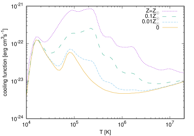
Figure 1: Cooling functions for optically-thin plasma with different metallicities (Sutherland & Dopita, 1993).

We adopted tabulated cooling data of optically-thin plasma by Sutherland & Dopita (1993) for the coronal region with $\rho\leq\rho_{\rm cr}=10^{-16}$ g cm^-3 and $T\geq 10^{4}$ K. We describe the reason for this choice of $\rho_{\rm cr}$ below at the section for the treatment at the transition region. Cooling functions, $\Lambda$ erg cm³s^-1, for different metallicities are available (Figure 1). Volumetric cooling rate $q_{\rm R}$ erg cm^-3s^-1 in Equation (10) is calculated via

$$q_{\rm R}=\Lambda nn_{\rm e},$$ (17)

where $n$ is ion number density and $n_{\rm e}$ is electron number density. We assumed fully ionized plasma with mean molecular weight, $\mu=0.6$, when deriving $n$ and $n_{\rm e}$ from $\rho$.

Chromosphere –Optically-thick cooling

The main coolants in the solar chromosphere are Mg II and Ca II with smaller contributions from H$\alpha$ and other metallic lines (Athay, 1976; Vernazza et al., 1981). These lines are not optically thin, and hence it is necessary to calculate detailed radiative transfer for the accurate treatment. In our original code for the solar wind (Suzuki & Inutsuka, 2005, 2006), instead of calculating radiation transfer, we adopted an empirical cooling rate, $q_{\rm R}=4.5\times 10^{9}\rho$ erg cm^-3s^-1, (Anderson & Athay, 1989) derived from observed chromospheric radiation. We extended this treatment to lower-metallicity stars.

In a zero-metallicity star, the chromospheric cooling is done solely by H$\alpha$ emission. The observation of the solar chromosphere shows that $\approx 20$% of the total chromospheric radiation is from H$\alpha$ (Athay, 1976; Linsky & Ayres, 1978). Following these arguments, we used a simple formula that describes metallicity-dependent chromospheric cooling rate,

$$q_{\rm R}=4.5\times 10^{9}\rho\left(0.2+0.8\frac{Z}{Z_{\odot}}\right){\rm erg\;cm^{-3}s^{-1}},$$ (18)

for the gas with $T\leq 10^{4}$K and $\rho\geq\rho_{\rm cr}$. We note that this simplified fitting formula needs to be calibrated by observations or radiative transfer calculations in future studies.

Transition Region –Interpolation

The transition region is located between the cool chromosphere and the hot corona, and its temperature is between $\approx 10^{4}$ K and $\approx 10^{6}$ K and the density is still higher than $\rho_{\rm cr}=10^{-16}$g cm^-3. We calculate radiation cooling in the transition region with $T>T_{\rm cr}$ and $\rho>\rho_{\rm cr}$ by interpolating Equations (17) & (18). The main reason why we chose $\rho_{\rm cr}=10^{-16}$g cm^-3 is somewhat technical; we can connect the two expressions for the radiative cooling near the bottom of the transition region almost independent from $Z$; equations (17) & (18) give the same value of $q_{\rm R}$ at $T=T_{\rm cr}=1.2\times 10^{4}$K for $Z=Z_{\odot}$ or at $T=T_{\rm cr}=1.1\times 10^{4}$K for $Z=0$. $T_{\rm cr}$ depends only weakly on $Z$, because the main coolant is hydrogen Ly$\alpha$ in this temperature range.

2.2.5 Initial Condition

We used the same MHD code described in §2.1.3 by replacing the Sun with the lower-metallicity stars in Table 1. We set up a static atmosphere with $T=T_{\rm eff}$; in the lower-altitude region with $\rho\gtrsim 10^{-10}\rho_{\rm ph}$, we adopted the hydrostatic density structure,

$$\rho_{\rm hs}=\rho_{\rm ph}\exp\left(-\frac{GM_{\star}}{c_{\rm s,eff}^{2}}\left(\frac{1}{R_{\star}}-\frac{1}{r}\right)\right),$$ (19)

while in the higher-altitude region, we set up density larger than $\rho_{\rm hs}$ in order to avoid unphysically fast Alfvén speed, which causes a troublesome short time-step when we update physical variables with time.

The simulations were carried out in dimensionless units. The simulation time is nondimensionalized via $t_{\rm sim}=R_{\star}/c_{\rm s,eff}$. We ran the simulations until $t_{\rm sim}=6$, which corresponds to 3-5 times the sound crossing time and $\gtrsim 10$ times the Alfvén crossing time of the simulation region.

3 Results

3.1 Time Evolution: 0.7$M_{\odot}$ Pop.III Star

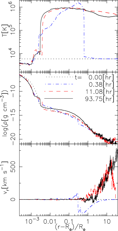
Figure 2: Time evolution of the atmospheric structure of the star with $M_{\star}=0.7M_{\odot}$ and $Z=0$. From the top to the bottom, $T$, $\rho$, and $v_{r}$ are displayed. Black dotted, blue dash-dotted, red dashed and black solid lines respectively correspond to the profiles at $t=0$, 0.38. 11.08, and 93.75 [hr] from the beginning of the simulation. Movie is also available as a supplementary file and at http://ea.c.u-tokyo.ac.jp/astro/Members/stakeru/research/movie/index.html.

Figure 2 demonstrates the time evolution of the atmosphere and wind of the zero-metal star with $M_{\star}=0.7M_{\odot}$. The simulation time, $t_{\rm sim}=6$, corresponds to $t\approx 100$ hr in the physical units for this case.

The top panel shows that the upper layer in $r\gtrsim 1.003R_{\star}$ is quickly heated up to the coronal temperature, $T\approx 10^{6}$ K, by the nonlinear dissipation of the Alfvénic waves from below. The main channel of the dissipation is the nonlinear mode conversion; the fluctuations of the magnetic pressure, $B_{\perp}^{2}$, with the Alfvénic waves excite density perturbations, which propagate as slow-mode MHD ($\approx$ sound) waves. They finally dissipate via shocks that are formed as a result of the steepening of the wavefronts. For the detail, see §4.3 and Suzuki & Inutsuka (2005, 2006), Suzuki et al. (2013), and Matsumoto & Suzuki (2012, 2014).

The red dash-dotted line at $t=11.08$ hr and black solid line at $t=93.75$ hr show that the temperature rises with height from $T\approx 4000$ K to $T\approx 10^{4}$ K. A nearly isothermal region with $T\approx 10^{4}$ K is formed by the Lyman-$\alpha$ cooling, which is seen as a peak just above $10^{4}$ K in the cooling curves in Figure 1. Therefore, below this quasi-isothermal region, the gas is partially ionized. Above this region, the gas is fully ionized and the temperature jumps up to $10^{6}$ K across the sharp transition region because the temperature range, $T\gtrsim 10^{5}$ K, is thermally unstable. Here, we should note that this Ly$\alpha$ plateau may not be realistic if ambipolar diffusion is properly taken into accuont (Fontenla et al., 1990) (see §4.1 for the validity of the ideal MHD approximation).

In the middle panel of Figure 2, the transition region is recognized as a sharp drop of the density to keep the pressure balance across this thin layer. In the chromosphere, the density slightly decreases from the initial value because the temperature decreases from the initial condition, $T=T_{\rm eff}$. In other words, the density decreases more rapidly with height because the pressure scale height ($\propto T$) is shorten. In contrast, the density in the corona gradually increases with time by chromospheric evaporation; the chromospheric material is heated by the downward thermal conduction from the corona and is supplied to the upper layer.

The bottom panel of Figure 2 shows that at the beginning the gas in the upper layer falls down to the surface (blue dash-dotted lines at $t=0.38$ hr), since the initial density is larger than $\rho_{\rm hs}$ (equation 19). However, Alfvénic waves propagating from the photosphere push back the infalling gas upward, and eventually stellar wind streams out in a quasi-steady manner. After $\approx$ 50 hr, which corresponds to $\approx$ twice the sound crossing time across the simulation region $R_{\star}<r\lesssim r_{\rm out}(=30R_{\star})$, the time-steady velocity profile is achieved.

$\rho$ and $v_{r}$ in the coronal region show fluctuations, most of which are longitudinal slow MHD (acoustic) wave-like perturbations excited by nonlinear mode conversion from Alfvénic waves (Kudoh & Shibata, 1999), discussed above. In contrast, $T$ does not exhibit fluctuations because the thermal conduction smooths out such small-scale perturbations.

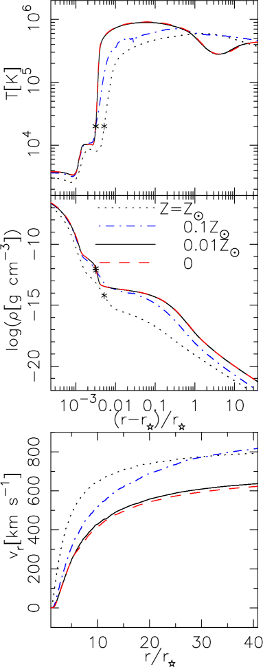
Figure 3: Comparison of the time-averaged stellar atmosphere and wind structures from 0.7 $M_{\odot}$ stars with different metallicities, $Z=Z_{\odot}$ (black dotted), $0.1Z_{\odot}$ (blue dash-dotted), $0.01Z_{\odot}$ (black solid), and $0$ (red dashed). From top to bottom, $T$, $\rho$, and $v_{r}$ are presented. In the top ($T$) and middle ($\rho$) panels, distance from the photosphere, $(r-R_{\star})/R_{\star}$ in the logarithmic scale is used to zoom in the low-atmospheric region. In the top panel ($v_{r}$), distance from the stellar center, $r/R_{\star}$, is shown in the linear scale for the horizontal axis. The asterisk in the top and middle panels indicate the location where $T=2\times 10^{4}$ K.

3.2 Dependence on Metallicity

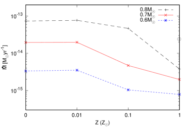
Figure 4: Dependence of mass loss rates by stellar winds from $0.8M_{\odot}$ (black dashed), $0.7M_{\odot}$ (red solid), and $0.6M_{\odot}$ (blue dotted) stars on metallicity. Note that the mass loss rate by the solar wind is also plotted on $Z=Z_{\odot}$.

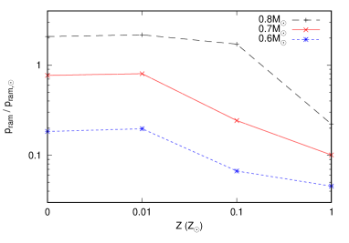
Figure 5: Dependence of ram pressure of stellar winds at $r=1$ au from $0.8M_{\odot}$ (black dashed), $0.7M_{\odot}$ (red solid), and $0.6M_{\odot}$ (blue dotted) stars on metallicity. $p_{\rm ram}$ is normalized by $p_{\rm ram}$ of the solar case.

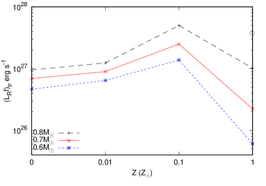
Figure 6: Dependence of the integrated radiation loss from the open magnetic regions in the UV and soft X-ray range, $(L_{\rm R}f)_{\rm tr}$ (equation 22), of $0.8M_{\odot}$ (black dashed), $0.7M_{\odot}$ (red solid), and $0.6M_{\odot}$ (blue dotted) stars on metallicity. $(L_{\rm R}f)_{\rm tr}$ of the solar case is also plotted on $Z=Z_{\odot}$.

We investigate how the atmospheres and winds depend on metallicity in this subsection. Figure 3 compares the atmospheric structures of 0.7$M_{\odot}$ stars with different metallicities. Here we focus on the time-averaged structures and took the average from $t_{\rm sim}=3$ to 6 after the quasi-steady-state structure is achieved. The $Z=0.01Z_{\odot}$ case shows the similar profiles of $T$, $\rho$, and $v_{r}$ to the zero-metallicity case in the three panels, which indicates that the effect of the different metallicities is negligible on the stellar winds for $Z\lesssim 0.01Z_{\odot}$.

The top panel of Figure 3 shows that hot coronae with temperature $\approx(0.5-1)\times 10^{6}$ K form in $r\gtrsim(1.005-1.01)R_{\star}$ in all the four cases. The temperature profiles are qualitatively similar each other: A nearly isothermal region with $T\approx 10^{4}$ K is formed by the Ly$\alpha$ cooling, and above that the temperature rapidly rises owing to the thermal instability (see §3.1). However, the peak temperature, $T_{\rm max}$, and its location depend on metallicity; lower $Z$ gives higher $T_{\rm max}$ that is located closer to the surface. This is because the efficiency of the cooling is suppressed for lower $Z$ (Figure 1) and denser gas located at lower altitudes can be heated up to higher temperature.

The middle panel of Figure 3 indicates that the density in the coronal region is higher for lower $Z$. This can be again explained by the suppression of the cooling. As a result, denser gas can be heated up to the coronal temperature (see also discussion on the energetics later in §3.3).

The bottom panel of Figure 3 shows that the dependence of the wind velocity on metallicity is weak, and the terminal velocity is roughly comparable to the escape velocity, $=\sqrt{2GM_{\star}/R_{\star}}$ ($\approx 650$ km s^-1 for these stars), whereas the wind velocity is slightly slower for lower $Z$ because denser material has to be lifted up and accelerated.

In the last two columns of Table 1, we show the time averaged mass loss rate,

$$\dot{M}=4\pi r^{2}\rho v_{r}f(r),$$ (20)

and terminal velocity, $v_{\rm t}=v_{r}$, at $r_{\rm out}(=30R_{\star})$, where $f(r_{\rm out})=1$ in equation (20). The difference of $\dot{M}$ for different $Z$ is mostly due to the difference of $\rho$ in the wind region. This is further connected to the difference of the density at the transition region marked by asterisks in the middle panel of Figure 3, where we define this location as the transition region, $r=r_{\rm tr}$, at $T=2\times 10^{4}$ K. For $M_{\star}=0.7M_{\odot}$, $\dot{M}$ of the $Z\leq 0.01Z_{\odot}$ stars is $\approx$ one order of magnitude larger than $\dot{M}$ of the solar metallicity star. This trend is qualitatively similar for different stellar masses, $0.6-0.8M_{\odot}$, as shown in Figure 4.

Figure 5 compares the ram pressures of stellar winds,

$$p_{\rm ram}=\rho v_{r}^{2},$$ (21)

of different $M_{\star}$ cases as a function of $Z$. Since $p_{\rm ram}$ decreases with $r$, we evaluated it at $r=1$ au, where we extrapolated $\rho$ and $v_{r}$ from $r=r_{\rm out}$ to $r=1$ au by assuming $\rho\propto r^{-2}$ for constant $v_{r}$. The vertical axis of Figure 5 is normalized by the value adopted from our solar case, $p_{\rm ram,\odot}$. Because $p_{\rm ram}\propto\dot{M}v_{\rm t}$ and $v_{\rm t}$ depends only weakly on $Z$, the general trend is very similar to that obtained for $\dot{M}$ (Figure 4). The ram pressure is an important parameter to determine the metal pollution on the surface of low-mass Pop.III stars (Tanaka et al., 2017, see also §1). Figure 5 shows that $p_{\rm ram}$ for the zero-metal stars with $M_{\star}\geq 0.7M_{\odot}$ is at least comparable to $p_{\rm ram}$ of the solar wind, and therefore, the surface pollution is negligible for these stars.

Figure 6 compares the integrated radiative coolings in the UV and soft X-ray range,

$$(L_{\rm R}f)_{\rm tr}=4\pi\int_{r_{\rm tr}}^{r_{\rm out}}q_{\rm R}fr^{2}dr,$$ (22)

of different $M_{\star}$ and $Z$ cases, where $r=r_{\rm tr}$ corresponds to the asterisks in Figure 3. The density in the coronal region of the $Z\leq 0.01Z_{\odot}$ cases is 1–2 orders of magnitude larger than that of the solar-metallicity case. The radiative flux in the corona is proportional to $\rho^{2}$ (see equation 17). Although the cooling efficiency, $\Lambda$ erg cm³s^-1, itself is much smaller for lower $Z$ (Figure 1), this is totally compensated by the enhanced density. As a result, $(L_{\rm R}f)_{\rm tr}$ of the $Z\leq 0.01Z_{\odot}$ cases is comparable ($M_{\star}=0.8M_{\odot}$) to or even considerably larger ($M_{\star}=0.7M_{\odot}$ and $0.6M_{\odot}$) than that of the solar metallicity case. $Z=0.1Z_{\odot}$ gives the maximum $(L_{\rm R}f)_{\rm tr}$ for each $M_{\star}$ case, because, compared to the cases with $Z\leq 0.01Z_{\odot}$, $\Lambda$ is considerably larger although the density is only slightly lower. We should cautiously note that equation (22) calculates the radiative flux from the open magnetic field region. In order to compare simulated radiative flux to observed UV and X-ray flux, we also need to take into account the contribution from closed loops, which is regarded to dominate that from open field regions.

3.3 Energetics

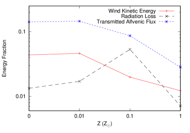
Figure 7: Comparison of fractional energy flux of the transmitted Alfvénic flux to the transition region (blue dotted), the radiation loss (black dotted), and the kinetic energy flux of the stellar wind (red solid) of the $0.7M_{\odot}$ stars, normalized by the input Alfvénic Poynting flux from the photosphere as a function of stellar metallicity.

We pursue the metallicity dependence from a more quantitative manner. In order to do so, we investigate the energetics of the stellar winds. After various modes of upgoing waves were injected from the photosphere, the only Alfvénic (transverse) waves survive into the coronal region, because compressive (longitudinal) waves rapidly dissipate by the formation of shocks as a result of the steepening of the wave fronts (e.g., Suzuki, 2002). Therefore, we focus on the variation of the Alfvénic Poynting flux with $r$, and study how the Poynting flux is converted to other types of energy fluxes.

The energy flux of Alfvénic waves along the $r$ direction is (Jacques, 1977; Suzuki et al., 2013)

$$F_{\rm A}=v_{r}\left(\rho\frac{v_{\perp}^{2}}{2}+\frac{B_{\perp}^{2}}{4\pi}\right)-B_{r}\frac{v_{\perp}B_{\perp}}{4\pi},$$ (23)

where the first term denotes the energy flux advected by background flow and the second term indicates the Poynting flux concerning magnetic tension. The second term dominates the first term in the low atmosphere where the average flow speed is much smaller than the Alfvén speed, $v_{\rm A}$, while the opposite is true in the wind region with $v_{r}>v_{\rm A}$. Therefore, the injected energy at the photosphere can be expressed as

$$F_{\rm A,0}\approx-\left(B_{r}\frac{v_{\perp}B_{\perp}}{4\pi}\right)_{0}\approx\rho_{\rm ph}\langle\delta v_{0}^{2}\rangle v_{\rm A,0},$$ (24)

where $\langle\cdots\rangle$ stands for the time-average. In order to exclude the effect of the adiabatic loss in a super-radially open flux tube, we introduce Alfvénic luminosity,

$$L_{\rm A}f=4\pi r^{2}fF_{\rm A}=\dot{M}\left(\frac{v_{\perp}^{2}}{2}+\frac{B_{\perp}^{2}}{4\pi\rho}\right)-\Phi_{B}\frac{v_{\perp}B_{\perp}}{4\pi},$$ (25)

where $\Phi_{B}=4\pi r^{2}fB_{r}$ is the total magnetic flux.

The Alfvénic waves that travel in the photosphere and chromosphere suffer reflection because the wave shape is deformed owing to the variation of $v_{\rm A}$ (Wentzel, 1978; Heinemann & Olbert, 1980; An et al., 1990; Suzuki & Inutsuka, 2006; Shoda & Yokoyama, 2016), and a small fraction of the input Poynting flux reaches the corona. We define the transmitted fraction $=(L_{\rm A}f)_{\rm tr}/(L_{\rm A}f)_{0}$, where the numerator is evaluated at $r=r_{\rm tr}$ and the denominator is evaluated at the photosphere, $r=R_{\star}$. A fraction of the transmitted Alfvénic energy flux is finally converted to the kinetic energy flux of the stellar wind,

$$L_{\rm K,out}=\dot{M}\frac{v_{{\rm t}}^{2}}{2}.$$ (26)

Figure 7 shows the fraction of the transmitted Alfvénic energy flux, $(L_{\rm A}f)_{\rm tr}/(L_{\rm A}f)_{0}$, (blue dotted), the radiation loss at and above the transition region, $(L_{\rm R}f)_{\rm tr}/(L_{\rm A}f)_{0}$, (black dashed) and the final kinetic energy flux of the stellar wind, $L_{\rm K,out}/(L_{\rm A}f)_{0}$ (red solid) of the $0.7M_{\odot}$ stars. We note that the transmitted Alfvénic energy flux equals to the sum of the radiation loss (equation 22), the kinetic energy flux (equation 26), the gravitational loss, and the Alfvénic energy flux outgoing from $r=r_{\rm out}$ (Suzuki et al., 2013), whereas the latter two are not shown.

The transmitted fraction is $\approx 14\%$ for the low-metallicity ($Z=0.01Z_{\odot}$ and 0) stars and it is $\approx 3\%$ for the solar metallicity star, which indicates that $\approx 86\%$ or $\approx 97\%$ of the input Alfvénic energy flux is reflected back downward to the photosphere in these cases. The transmitted fraction is larger for lower-metallicity stars because of the difference of the location of the transition region. In lower-metallicity stars, dense gas can be heated up to the coronal temperature because of the suppressed cooling, and therefore, the density at the transition region is higher. As a result, the Alfvénic waves travel a shorter distance with a smaller density contrast from the photosphere to the transition region (the middle panel of Figure 3), and they suffer less reflection through the propagation in the chromosphere.

This is, in a sense, a positive feedback with respect to the heating by the dissipation of Alfvénic waves. When metallicity decreases, denser gas can be heated up by the suppressed radiation cooling, which further reduces the reflection of Alfvénic waves. This raises the transmitted Alfvénic Poynting flux to the corona, which further enhances the heating in the corona.

Since the transmitted fraction is quite small ($\approx 3\%$) in the solar metallicity star, the fraction of $L_{\rm K,out}$ is also small, $\approx 1.2\%$. The fraction of $(L_{\rm R}f)_{\rm tr}$ is also tiny; the radiation cooling, which is $\propto\rho^{2}$, is not substantial because the density at the transition region (and corona) is already much smaller than in the cases with lower $Z$.

If we compare the case with $Z=0.1Z_{\odot}$ to the cases with $Z\leq 0.01Z_{\odot}$, a larger fraction is converted to $(L_{\rm R}f)_{\rm tr}$ than to $L_{\rm K,out}$, because $\Lambda$ in $10^{5}$K $\lesssim T\lesssim 10^{6}$K is larger by a factor of 5-10 (Figure 1). As a result, the fraction converted to the wind is $L_{\rm K,out}\approx 2\%$, which is considerably smaller than the fraction $\approx 4.5\%$ obtained in the lower $Z$ cases.

Table 1 and Figure 4 show that $\dot{M}$ of $Z\leq 0.01Z_{\odot}$ is 10 times and $\dot{M}$ of $Z=0.1Z_{\odot}$ is 2.4 times larger than $\dot{M}$ of $Z=Z_{\odot}$ for $M_{\star}=0.7M_{\odot}$. These values are larger than the estimates from the energy conversion efficiency, $L_{\rm K,out}/(L_{\rm A}f)_{0}$, we have discussed above. This is mainly because the input Alfvénic energy, $(L_{\rm A}f)_{0}$, from the photosphere (equation 24) is larger for lower $Z$ on account of the moderately larger convective flux ($\propto T_{\rm eff}^{4}$; see equation 15 and Table 1); $(L_{\rm A}f)_{0}$ of $Z\leq 0.01Z_{\odot}$ is 1.7 times and $(L_{\rm A}f)_{0}$ of $Z=0.1Z_{\odot}$ is 1.5 times larger than $(L_{\rm A}f)_{0}$ of $Z=Z_{\odot}$. In addition, the terminal velocity, $v_{\rm t}$, of the $Z\leq 0.01Z_{\odot}$ cases is $\approx 20\%$ slower than $v_{\rm t}$ of the $Z=Z_{\odot}$ case. Therefore, the difference ($\approx$ a factor of 10) of $\dot{M}$ between $Z\leq 0.01Z_{\odot}$ and $Z=Z_{\odot}$ is larger than the difference ($\approx$ a factor of 6-7) of $L_{\rm K,out}$ (equation 26).

3.4 Scaling Relation for $\dot{M}$

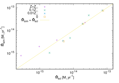
Figure 8: Comparison of the mass loss rate from the scaling relation, $\dot{M}_{\rm scl}$ (equation 39), and the mass loss rate of the simulations, $\dot{M}_{\rm sim}$. The normalization of the scaling is from the solar value $\eta_{\rm scl}=2.22\times 10^{-14}M_{\odot}$yr^-1 (Table 1). Different symbols correspond to different metallicities. As for the solar metallicity cases, we show the result of $M_{\star}=M_{\odot}$ in addition to $M_{\star}=0.6$, 0.7, & 0.8$M_{\odot}$.

In this subsection we derive a simple scaling relation of $\dot{M}$ from our simulations, following the energetics argument in §3.3. Figure 7 indicates that the wind kinetic energy is almost proportional to the transmitted Alfvénic Poynting flux to the corona, namely, $L_{\rm K,out}\propto(L_{\rm A}f)_{\rm tr}$. The terminal velocity can be roughly scaled by the escape velocity, $v_{\rm t}\sim\sqrt{2GM_{\star}/R_{\star}}$, and then, we have

$$\dot{M}\propto(L_{\rm A}f)_{0}c_{\rm T}(R_{\star}/M_{\star}),$$ (27)

where $c_{\rm T}=(L_{\rm A}f)_{\rm tr}/(L_{\rm A}f)_{0}$ is the transimissivity of Alfvénic waves from the photosphere to the corona. Using equations (15) & (24), we get the dependence of $(L_{\rm A}f)_{0}$ on stellar parameters:

$$(L_{\rm A}f)_{0} = 4\pi R_{\star}^{2}fF_{\rm A,0}$$ (28)

$$\propto \rho_{\rm ph}^{1/2}\delta v_{0}^{2}(B_{r}f)_{0}R_{\star}^{2}$$

$$= (\rho_{\rm ph}\delta v_{0}^{3}R_{\star}^{2})^{2/3}\rho_{\rm ph}^{-1/6}R_{\star}^{2/3}$$

$$\propto L^{2/3}\rho_{\rm ph}^{-1/6}R_{\star}^{2/3},$$

where we used the assumption, $(B_{r}f)_{0}=$const. in equation (5).

After Alfvénic waves are excited from the photosphere, these waves, which are affected by dissipation and reflection, travel upward. Determining $c_{\rm T}$ is a very difficult task because it is not simple to properly take into account these processes with nonlinear effects. Here we consider the situation in which the reflection is a dominant process that controls $c_{\rm T}$. In the stellar atmosphere, both density and magnetic field strength change rapidly with height. As a result, the Alfvén velocity also varies. Alfvénic waves with wavelength, $\lambda$, longer than the variation scale of $v_{\rm A}$ are subject to reflection because of the deformation of the wave shape (Suzuki & Inutsuka, 2006; Shoda & Yokoyama, 2016). In the long-wavelength limit, $\lambda\gg|\frac{dr}{d\ln v_{\rm A}}|$, we can derive the transmitted wave amplitude from a region I with density $\rho_{\rm I}$ to a region II with $\rho_{\rm II}$ as follows (Hollweg, 1984; Verdini et al., 2012):

$$\delta v_{\perp,{\rm II}}=\frac{2}{1+\sqrt{\rho_{\rm II}/\rho_{\rm I}}}\delta v_{\perp,{\rm I}}$$ (29)

Using this transmissivity for velocity amplitudes, we can estimate $c_{\rm T}$ from the photosphere to the corona:

$$c_{\rm T}=\frac{(\rho\delta v_{\perp}^{2}v_{\rm A,tr}fr^{2})_{\rm tr}}{\rho_{\rm ph}\delta v_{0}^{2}v_{\rm A,0}f_{0}R_{\star}^{2}}=\frac{4\sqrt{\rho_{\rm ph}/\rho_{\rm tr}}}{(\sqrt{\rho_{\rm ph}/\rho_{\rm tr}}+1)^{2}}\approx 4\sqrt{\frac{\rho_{\rm tr}}{\rho_{\rm ph}}},$$ (30)

where $\rho_{\rm tr}$ is the density at the bottom of the transition region at which $T=T_{\rm tr}$($=2\times 10^{4}$K). We used $(\sqrt{\rho}v_{\rm A}fr^{2})_{\rm tr}=\sqrt{\rho_{\rm ph}}v_{\rm A,0}f_{0}R_{\star}^{2}$ derived from the conservation of magnetic flux, equation (4), and $\rho_{\rm ph}\gg\rho_{\rm tr}$ for the last approximate equality.

$\rho_{\rm tr}$ is determined by the balance between heating and conductive and radiative cooling (Rosner et al., 1978); the heating in the transition region and the low corona is mainly lost by the downward thermal conduction to the chromosphere, in addition to the radiative cooling. When heating increases, the enhanced downward thermal conduction makes cool chromospheric materials evaporate to the corona, which leads to larger $\rho_{\rm tr}$. Since the conductive flux is finally lost by the radiation in the transition region and the upper chromosphere, we can assume that the heating by the wave dissipation, $(\rho\delta v_{\perp}^{2}v_{\rm A})_{\rm tr}/\tau_{\rm dis}$, is balanced by $q_{\rm R}$ in equation (10). We adopt optically thin cooling, equation (17), and then, $q_{\rm R}\propto\rho^{2}\Lambda$. Introducing a dissipation length, $l_{\rm dis}$, we can write the heating rate by the dissipation of Alfvénic waves as $\rho\delta v_{\perp}^{2}v_{\rm A}/l_{\rm dis}$. Then, we obtain an equation that describes the energy balance at and above the transition region,

$$\int_{r_{\rm tr}}^{r_{\rm max}}dr\left(\frac{\rho}{\mu m_{\rm u}}\right)^{2}\Lambda\sim\int_{r_{\rm tr}}^{r_{\rm max}}dr\frac{\rho\delta v_{\perp}^{2}v_{\rm A}}{l_{\rm dis}},$$ (31)

where the integration is done from the bottom of the transition region, $r=r_{\rm tr}$, to the location, $r=r_{\rm max}$, that gives the maximum temperature. This relation indicates that enhanced heating and/or reduced cooling leads to higher $\rho_{\rm tr}$ owing to the efficient chromospheric evaporation, as explained above. We can transform the left-hand-side of equation (31) as

$$\int_{r_{\rm tr}}^{r_{\rm max}}dr\rho^{2}\Lambda\equiv\langle\Lambda\rangle_{\rho^{2}}\int_{r_{\rm tr}}^{r_{\rm max}}dr\rho^{2}\approx\langle\Lambda\rangle_{\rho^{2}}\rho_{\rm tr}^{2}H_{\rm tr},$$ (32)

where for the last approximate equality we used the fact that the integral of density is heavily weighted on the smaller $r$ side near $r=r_{\rm tr}$ because the density rapidly decreases with $r$, and $H_{\rm tr}=k_{\rm B}T_{\rm tr}/\mu m_{\rm u}g$ is the pressure scale height measured for $T=T_{\rm tr}$($=2\times 10^{4}$K). We put $\rho^{2}$ for the subscript of $\langle\Lambda\rangle$ to explicitly show that this is the ${\rho}^{2}$-weighted cooling function.

In our simulations, Alfvénic waves dissipate via nonlinear processes (see §4.3). In this case, we can model that the dissipation rate is proportional to nonlinearity, $\delta v_{\perp}/v_{\rm A}$, and that

$$l_{\rm dis}\sim\lambda(\delta v_{\perp}/v_{\rm A})^{-1}\sim\frac{v_{\rm A}^{2}}{\omega\delta v_{\perp}},$$ (33)

where we used $\lambda\sim v_{\rm A}/\omega$. From equation (29), we have

$$\delta v_{\perp,{\rm tr}}\approx 2\delta v_{0}\propto\delta v_{0}$$ (34)

The integration of the right-hand-side of equation (31) is also weighted near $r=r_{\rm tr}$ similarly to the left-hand side (equation 32) because the volumetric heating rate is proportional to $\rho$. Substituting equations (33) & (34) into the the right-hand-side of equation (31), we have

$$\int_{r_{\rm tr}}^{r_{\rm max}}dr\frac{\rho\delta v_{\perp}^{2}v_{\rm A}}{l_{\rm dis}}\approx\frac{\rho_{\rm tr}\delta v_{0}^{3}\omega}{v_{\rm A,tr}}H_{\rm tr}$$ (35)

Applying equations (32) & (35) to equation (31), we obtain

$$\rho_{\rm tr}^{2}\langle\Lambda\rangle_{\rho^{2}} \propto \rho_{\rm tr}\delta v_{0}^{3}\omega/v_{\rm A,tr}$$ (36)

$$\sim \rho_{\rm tr}^{3/2}T_{\rm eff}^{4}\rho_{\rm ph}^{-1}M_{\star}R_{\star}^{-2}T_{\rm eff}^{-1/2}$$

$$= \rho_{\rm tr}^{3/2}T_{\rm eff}^{7/2}\rho_{\rm ph}^{-1}M_{\star}R_{\star}^{-2},$$

where we used equations (15) & (16), and $v_{\rm A,tr}\propto\rho_{\rm tr}^{-1/2}$ because we can assume $B_{r,{\rm tr}}\sim(Bf)_{0}=$const. As a result, we get the scaling of $c_{\rm T}$,

$$c_{\rm T}\propto\langle\Lambda\rangle_{\rho^{2}}^{-1}T_{\rm eff}^{7/2}M_{\star}R_{\star}^{-2}\rho_{\rm ph}^{-3/2}.$$ (37)

From equation (12), we adopt

$$\rho_{\rm ph}\propto M_{\star}^{2/3}R_{\star}^{-4/3}T_{\rm eff}^{-2},$$ (38)

where we neglected the weak dependence on metallicity. Substituting equations (28), (37) & (38) into equation (27), we finally have the scaling of $\dot{M}$:

$$\dot{M} \propto \langle\Lambda\rangle_{\rho^{2}}^{-1}LR_{\star}^{-1}T_{\rm eff}^{13/6}\rho_{\rm ph}^{-5/3}$$ (39)

$$\propto \langle\Lambda\rangle_{\rho^{2}}^{-1}LR_{\star}^{11/9}M_{\star}^{-10/9}T_{\rm eff}^{11/2}$$

The cooling function, $\Lambda$, depends on $Z$ (Figure 1). If we focus on gas in the transition region with $10^{4}\lesssim T\lesssim 10^{6}$ K, $\Lambda$ does not depend on $Z$ for $T\lesssim 10^{4.5}$K because the main coolant is hydrogen atoms, while $\Lambda$ strongly depends on $Z$ for $T\gtrsim 10^{4.5}$K. Although the former temperature range is quite narrow, it is not negligible for the $\rho^{2}$-weighted cooling, $\langle\Lambda\rangle_{\rho^{2}}$ because it is biased on the lower temperature side. Considering this situation, we adopt a weak dependence on $Z$ with a floor in $Z<0.01Z_{\odot}$, which can reasonably explain our simulation results:

$$\langle\Lambda\rangle_{\rho^{2}}\propto\left[\max\left(\frac{Z}{Z_{\odot}},0.01\right)\right]^{\frac{1}{5}}.$$ (40)

Applying equation (40) to equation (39), we finally obtain an equation that predicts mass loss rate from stellar basic parameters:

$$\dot{M}_{\rm scl} = \eta_{\rm scl}\frac{L}{L_{\odot}}\left(\frac{R_{\star}}{R_{\odot}}\right)^{\frac{11}{9}}\left(\frac{M_{\star}}{M_{\odot}}\right)^{-\frac{10}{9}}\left(\frac{T_{\rm eff}}{T_{\rm eff,\odot}}\right)^{\frac{11}{2}}$$ (41)

$$\times\left[\max\left(\frac{Z}{Z_{\odot}},0.01\right)\right]^{-\frac{1}{5}},$$

where the normalization is adopted from the solar mass loss rate of our simulation, $\eta_{\rm scl}=\dot{M}_{\odot}$($=2.22\times 10^{-14}M_{\odot}$yr^-1; Table 1).

It is worth comparing this relation to previous works. The famous Reimers’ relation (Reimers, 1975) was derived from simple energetics,

$$\dot{M}_{\rm Reimers}=\eta_{\rm Reimers}\frac{(L/L_{\odot})(R_{\star}/R_{\odot})}{M_{\star}/M_{\odot}},$$ (42)

where the original normalization, $\eta_{\rm Reimers}=4\times 10^{-13}M_{\odot}$yr^-1, was adopted as a standard value for red supergiants.

Schröder & Cuntz (2005) modified this relation by including an mechanical energy input and a chromospheric radius, which is located far above the photosphere in red giant stars, and derive

$$\dot{M}_{\rm SC05}=\eta_{\rm SC05}\frac{(L/L_{\odot})(R_{\star}/R_{\odot})}{M_{\star}/M_{\odot}}\left(\frac{T_{\rm eff}}{4000\;{\rm K}}\right)^{3.5}\left(1+\frac{g_{\odot}}{4300g}\right),$$ (43)

where $\eta_{\rm SC05}=8\times 10^{-14}M_{\odot}$yr^-1 was introduced as a standard normalization for red giants. The power-law indices of $R_{\star}$, $M_{\star}$, and $T_{\rm eff}$ in equation (41) are slightly different from those in equation (43). The biggest difference is that our relation explicitly considers the effect of metallicity. If we are to apply our relation to metal-poor red giants, it is probably better to include the explicit dependence on $g$ presented in equation (43)

Figure 8 compares $\dot{M}_{\rm scl}$ derived from equation (41) and $\dot{M}_{\rm sim}$ of the numerical simulations. Although we took several crude simplifications, the derived scaling relation explains the overall trend of the simulation results. The fitting of either higher-mass ($M_{\star}=0.8M_{\odot}$) or lower-metallicity ($Z\leq 0.01Z_{\odot}$) cases is quite nice. On the other hand, $\dot{M}_{\rm scl}$ of lower-mass ($M_{\star}\leq 0.7M_{\odot}$) solar metallicity stars underestimates $\dot{M}_{\rm sim}$, while $\dot{M}_{\rm scl}$ of $M_{\star}=0.6M_{\odot}$ and $Z=0.1Z_{\odot}$ slightly overestimates $\dot{M}_{\rm sim}$.

4 Discussion

4.1 Magnetic Diffusion

We should critically check the validity of the ideal MHD approximation we have assumed in this paper, because the gas in the photosphere and chromosphere is not fully ionized. While in the solar metallicity gas metals with low ionization potential dominantly supply electrons, in the zero-metal gas the hydrogen is almost the sole source of electrons in the photosphere and chromosphere because the helium stays as neutral. On the other hand, the effective temperature of a lower metallicity star is higher than that of a higher metallicity star (Table 1). If we compare two stars with the same $M_{\star}$ but different $Z$, the former effect decreases the ionization degree of the lower $Z$ star, while the latter effect increases it. If we take the four stars with $M_{\star}=0.7M_{\odot}$ in Table 1 for example, these stars give similar ionization degrees, $x_{e}\sim 10^{-5}-10^{-4}$ at the photosphere under the local-thermodynamical-equilibrium condition, because the two effects are almost canceled out each other.

In the high-density condition, Ohmic dissipation is the dominant damping mechanism. Ohmic resistivity (magnetic diffusivity), $\chi_{\rm O}$, by electron-neutral collision can be estimated (Blaes & Balbus, 1994) as

$$\chi_{\rm O}\approx 230\sqrt{T}/x_{e}\;{\rm cm^{2}s^{-1}}.$$ (44)

We evaluate how the Ohmic dissipation affects the propagation of Alfvén waves by a magnetic Reynolds number. In fluid mechanics, a Reynolds number, $Re$, which is defined as the ratio of an inertial term to a viscous term, is often used as a measure of dissipation; flow tends to be laminar for $Re\lesssim 1$ and turbulent for $Re\gg 1$. In order to examine the propagation of Alfvénic Poynting flux, an inertial term is replaced by a term derived from Alfvén waves,

$$C_{\rm A}=\lambda v_{\rm A}=10^{14}\left(\frac{\lambda}{1000\;{\rm km}}\right)\left(\frac{v_{\rm A}}{10\;{\rm km\;^{-1}}}\right)\;{\rm cm^{2}s^{-1}},$$ (45)

where $\lambda(=v_{\rm A}/\omega)$ and $v_{\rm A}$ were normalized by typical quantities in the photosphere and chromosphere. In the zero-metal star with $M_{\star}=0.7M_{\odot}$, we inject perturbations in the frequency range between $\omega_{\rm max}^{-1}\approx 10$ s and $\omega_{\rm min}^{-1}\approx 1000$ s. $\lambda=1000$ km corresponds to the central value, $\omega^{-1}=100$ s.

Under the thermal equilibrium, the Saha equation for the ionization of hydrogen atoms gives $x_{e}\propto 1/\sqrt{\rho}$ (e.g., Gray, 1992). Hence, the Ohmic diffusion affects most severely at the densest location, namely the photosphere (inner boundary) in our simulations. From equations (44) and (45), we estimate a magnetic Reynolds number by the Ohmic dissipation at the photosphere of the zero-metal star with $M_{\star}=0.7M_{\odot}$,

$$Re_{\rm O} = \frac{C_{\rm A}}{\chi_{\rm O}}$$ (46)

$$\approx 4.0\times 10^{5}\left(\frac{x_{e}}{7\times 10^{-5}}\right)\left(\frac{T}{5842\;{\rm K}}\right)^{-1/2}$$

$$\hskip 28.45274pt\left(\frac{\lambda}{1000\;{\rm km}}\right)\left(\frac{v_{\rm A}}{10\;{\rm km\;s^{-1}}}\right),$$

where the normalization of $x_{e}=7\times 10^{-5}$ is adopted from (the interpolation of) ATLAS atmospheres, and this is consistent with the value derived from the Saha equation for the ionization of hydrogen atoms. Although $Re_{\rm O}$ becomes an order of magnitude smaller for $\omega_{\rm max}^{-1}\approx 10$ s, it still gives $Re_{\rm O}\approx 4.0\times 10^{4}\gg 1$. Lower-mass stars give lower ionization because the temperature is lower; the zero-metal star with $0.6M_{\odot}$ gives $x_{e}=1.2\times 10^{-5}$. $Re_{\rm O}$ estimated from this $x_{e}$ is still much larger than unity. Therefore, we can conclude that the Alfvén waves we have considered are not so affected by the Ohmic diffusion.

In the low-density condition, ambipolar diffusion between charged particles and neutral particles is the main damping mechanism. Ambipolar diffusivity, $\chi_{\rm A}$, can be estimated from $x_{e}$ and ion-neutral collision rate (Nakano & Umebayashi, 1986; Susa et al., 2015) as

$$\chi_{\rm A}=\frac{(m_{i}+m_{n})B^{2}}{4\pi\langle\sigma v\rangle_{\rm in}\rho_{i}\rho_{n}},$$ (47)

where the subscript $i$ and $n$ denote ions and neutrals, respectively, and $\langle\sigma v\rangle_{\rm in}=1.9\times 10^{-9}$cm³s^-1 is ion-neutral collision rate per number density (Draine et al., 1983). Substituting $m_{i}=m_{\rm H}$ and $m_{n}=\mu m_{\rm H}$ with $\mu=1.3$, we can derive for $x_{e}\ll 1$

$$\chi_{\rm A} \approx 2.1\times 10^{-16}\frac{B^{2}}{\rho^{2}x_{e}}\;{\rm cm^{2}s^{-1}}$$ (48)

$$= 2.1\times 10^{11}\left(\frac{B}{100\;{\rm G}}\right)^{2}$$

$$\hskip 28.45274pt\left(\frac{\rho}{10^{-10}{\rm g\;cm^{-3}}}\right)^{-2}\left(\frac{x_{e}}{10^{-3}}\right)^{-1}\;{\rm cm^{2}s^{-1}},$$

where the normalizations are adopted from the physical quantities at $T\approx 5000$ K in the mid to upper chromosphere; the ambipolar diffusion is expected to affect the propagation of Alfvén waves most substantially in this region because the density becomes low but the ionization is still not high there.

From equations (45) and (48), we can estimate a magnetic Reynolds number by the ambipolar diffusion in the mid to upper chromosphere,

$$Re_{\rm A} = \frac{C_{\rm A}}{\chi_{\rm A}}$$ (49)

$$\approx 4.8\times 10^{2}\left(\frac{B}{100\;{\rm G}}\right)^{2}\left(\frac{\rho}{10^{-10}{\rm g\;cm^{-3}}}\right)^{-2}$$

$$\hskip 28.45274pt\left(\frac{x_{e}}{10^{-3}}\right)^{-1}\left(\frac{\lambda}{1000\;{\rm km}}\right)\left(\frac{v_{\rm A}}{10\;{\rm km\;s^{-1}}}\right).$$

This estimate is again for the Alfvén wave with $\omega^{-1}=100$ s, and for higher-frequency waves, $\omega_{\rm max}^{-1}=10$ s, $Re_{\rm A}=48$. The ionization degree is lower for lower-mass stars. For example, $Re_{\rm A}\approx 10$ for the Alfvén wave with $\omega=\omega_{\rm max}$ in $M_{\star}=0.6M_{\odot}$. Although $Re_{\rm A}$ is still larger than unity, the Alfvén waves in the higher-frequency range within the injected spectral band are regarded to be subject to damping. For more realistic treatment for these stars in our future studies, we need to take into account ambipolar diffusion in the chromosphere.

4.2 Magnetic Activity of Metal-poor Stars

A crucial assumption of our work is that we determined the properties of the magnetic flux tubes by extrapolating the parameters of a typical magnetic flux tube on the Sun, because we have no direct observational information on the magnetic field of low-mass Pop. II/III stars. Although a Pop.III star has not been discovered, we infer some clues of magnetic activity of low-mass Pop.II stars from observations by UV and X-ray radiation.

Ottmann et al. (1997) analyzed X-ray observations of 86 Pop.II binaries from the ROSAT all-sky survey. They detected X-rays from the stellar coronae of 13 systems of which luminosity $10^{27}$erg s^-1$<L_{X}<2\times 10^{31}$erg s^-1 with only upper limits for the other 73 systems. Although the expected median X-ray luminosity is not so high, $L_{X}\leq 10^{28.1}$erg s^-1, if both detections and non-detections are all considered, a very metal-poor binary, HD89499, with [Fe/H]$=-2.1$ emits $L_{X}=1.3\times 10^{31}$erg s^-1, which is much larger than the X-ray luminosity of the Sun, $L_{X,\odot}\sim 10^{27}$erg s^-1 (e.g., Güdel, 2004). Moreover, the temperature of the coronal plasma of HD89499 was found to be very high, $T=2.6\times 10^{7}$K, from ASKA and ROSAT observations (Fleming & Tagliaferri, 1996).

Recently, X-ray was detected in the nearest Pop.II star with [Fe/H]$=-0.86$, the Kapteyn’s star, which is a single star having planets (Guinan et al., 2016). The detected X-ray luminosity is $L_{X}=(2.4-6.0)\times 10^{26}$erg s^-1. Since the stellar mass is small, $M_{\star}=0.281M_{\odot}$, the bolometric luminosity is only $L_{\rm bol}=0.012L_{\odot}$. Therefore, the normalized X-ray luminosity is $L_{X}/L_{\rm bol}\sim 10^{-5}$, which is quite large compared to the solar value, $L_{X}/L_{\rm bol}\sim 10^{-7}-10^{-6}$, even though this star is quite old with the age $\approx 11.5$ Gyr.

These observations indicate that at least some portions of metal-poor stars exhibit high magnetic activity. Although the detailed properties of the magnetic field are unknown and it is not well understood how the dynamo process depends on metallicity, we expect that a sizable fraction of metal-poor stars possesses magnetic field of which strength is comparable to or larger than the solar value. Therefore, we think it is reasonable to assume the magnetic flux tubes for metal-deficient stars introduced in §2.2, whereas detailed wind properties also depend on the filling factor, $f_{0}$, of open magnetic field (Suzuki, 2006).

We determined the velocity amplitude, $\delta v_{0}$, at the photosphere from the convective flux by equation (15). Although this estimate is expected to be independent from metallicity, we should note that the transverse fluctuation of magnetic flux tubes may depend on metallicity. Musielak & Ulmschneider (2002) analytically evaluated the energy flux of vertically oriented magnetic flux tubes. Their result shows that the energy flux of transverse fluctuations is independent from metallicity for hotter stars with $T_{\rm eff}\gtrsim 6000$ K, while it depends almost linearly on $Z$ for cooler stars with $T_{\rm eff}\lesssim 4000$ K. Our adopted $\delta v_{0}$ is reasonable for the cases with $M_{\star}\geq 0.7M_{\odot}$, while it may be overestimated for the cases with $M_{\star}=0.6M_{\odot}$.

We mention the effect of stellar rotation, which have not been taken into account in this paper. Stellar rotation affects the stellar atmosphere and wind in two ways. First, if the rotation is fast, it directly affects the velocity profile of the wind by the direct centrifugal acceleration (Weber & Davis, 1967). Second, stellar rotation influences the differential rotation in the surface convection zone (Brun & Toomre, 2002; Hotta & Yokoyama, 2011), and therefore, it probably affects the amplification of magnetic field there. Low-mass stars lose their angular momentum throughout the pre-main sequence and main sequence phases by magnetized stellar winds (Weber & Davis, 1967; Hirose et al., 1997; Vidotto et al., 2009; Pinto et al., 2011; Matt et al., 2012; Jardine et al., 2013; Réville et al., 2015; Johnstone et al., 2015). In the present universe, long-lived low-mass Pop.III/II stars are probably slow rotators as a result of the magnetic braking. Therefore, the first effect of the centrifugal acceleration of the wind is unimportant for these stars. On the other hand, the second effect of the dynano action is probably subect to the stellar rotation because the surface magnetic flux depends on the rotation rate (See et al., 2018).

4.3 Wave Dissipation

Both the magnetic pressure associated with propagating Alfvénic waves and the gas pressure of the stellar coronae contribute to driving the stellar winds from our low-mass Pop.II/III stars. The dissipation of the Alfvénic waves is a key in driving the stellar winds because it controls the gas pressure through the heating and the gradient of the Alfvénic magnetic pressure (Suzuki, 2004; Suzuki & Inutsuka, 2006). In our simulations the injected Alfvénic Poynting flux from the surface mainly dissipates via nonlinear excitation of longitudinal waves (Kudoh & Shibata, 1999; Suzuki & Inutsuka, 2005; Nariyuki & Hada, 2006, 2007; Murawski & Zaqarashvili, 2010; Vasheghani Farahani et al., 2011). Density fluctuations, which are regarded as longitudinal waves, are actually detected in the solar wind by radio scintillation measurements using AKATSUKI (Miyamoto et al., 2014). However, since our simulations are restricted to the simple 1D geometry, other dissipation channels may be also important in more realistic situations. We here briefly discuss wave dissipation mechanisms that we do not take into account, referring to works for the solar corona and wind.

The injected Alfvénic perturbation excites shear Alfvén waves with random polarization in our simulations. However, if the effect of a magnetic flux tube is directly considered, torsional Alfvén waves also have to be treated, because the dissipation characters of shear and torsional modes are slightly different (Nakariakov et al., 2000; Vasheghani Farahani et al., 2012). In realistic 3D circumstances, Alfvén waves also dissipate via turbulent cascade (Matthaeus et al., 1999; Verdini & Velli, 2007; Cranmer et al., 2007; Lionello et al., 2014; Adhikari et al., 2015; Yang et al., 2016; van Ballegooijen & Asgari-Targhi, 2016; Tenerani & Velli, 2017), while the mode conversion to compressive waves will be suppressed because propagating waves are not confined in a single flux tube.

It is still unclear how these processes modify the dissipation rate in a quantitative sense. However, we can infer how the assumption of the 1D flux tubes affects the wave dissipation from the comparison between simulations with different dimensions. 2.5D MHD simulations by Matsumoto & Suzuki (2012, 2014) show that the dissipation through the generation of compressive waves is suppressed, compared to 1.5D simulations by Suzuki & Inutsuka (2005, 2006). However, this suppression is almost exactly compensated by the resistive dissipation by shearing motion between neighboring magnetic field lines (Heyvaerts & Priest, 1983). As a result, the total heating rates by the dissipation of Alfvén waves are not so different at least between the 1.5D and 2.5D simulations. If this tendency can be extended to 3D simulations, our results of the overall wave heating and the basic properties of the atmospheric structures are expected to be reasonable.

5 Summary

We investigated the structure of atmospheres and winds in open magnetic field regions on low-mass stars with various metallicities. We injected velocity fluctuations, of which the amplitude is evaluated from the convective flux, from the location at $T=T_{\rm eff}$ and solved MHD equations with radiative cooling and thermal conduction in super-radially open one-dimensional magnetic flux tubes. By the dissipation of the Alfvénic waves traveling from the photosphere hot coronae with $>0.5\times 10^{6}$K are formed and coronal winds stream out in all the simulated stars with $M_{\star}=(0.6-0.8)M_{\odot}$ and $Z=(0-1)Z_{\odot}$. However, the properties of the coronae and winds depend on metallicity.

Denser gas can be heated up to the coronal temperature for lower metallicity, because the radiation cooling is suppressed. As a result, the transition region that separates the cool chromosphere and the hot corona is located at a lower height with higher density. The coronal density of the stars with $Z\leq 0.01Z_{\odot}$ is 1-2 orders of magnitude higher than the coronal density of the solar-metallicity star with the same stellar mass.

The difference between the density at the photosphere and the density in the corona is smaller for lower-metallicity stars. Because density difference determines the reflection of Alfvénic waves, the smaller density contrast leads to a larger transmissivity of the Alfvénic waves to the corona, which enhances the heating in the corona. This enhanced heating, combined with the suppressed radiation cooling, can explain the larger coronal density in lower-metallicity stars. The coronal X-ray flux, which is proportional to $\rho^{2}$, is also larger for lower metallicity, even though the cooling efficiency, $\Lambda$ (erg cm³s^-1), is smaller.

We should note that this discussion is based on our simulations in open magnetic field regions. In reality, X-rays are considered to come dominantly from closed field regions on a stellar surface, because denser plasma can be confined in closed loops. Therefore, for quantitative estimates of X-rays, closed magnetic loops need to be taken into account in our future studies.

The mass loss rate of the low-metallicity stars with $Z\leq 0.01Z_{\odot}$ is $(4.5-20)$ times larger than that of the solar-metallicity star with the same mass, because of the larger coronal density. In terms of the energetics, a larger fraction of the input Alfvénic wave energy is transferred to the kinetic energy of the stellar wind because of the suppression of the wave reflection and the radiation loss.

It is interesting to note that the dependence of the mass loss rate on metallicity is opposite to the trend for luminous stars. Stellar winds from massive main sequence stars are driven by the radiation pressure acting on metallic lines in the UV range (Lucy & Solomon, 1970; Castor et al., 1975). The radiation pressure on dust grains plays an important role in stellar winds from AGB stars (Bowen, 1988; Ohnaka et al., 2016). These contributions are reduced for decreasing metallicity, and therefore, the mass loss rate of these stars is smaller for lower metallicity (Kudritzki, 2002; Tashibu et al., 2017) The main difference of less luminous stars we have studied in this paper from these luminous stars is that the radiation acts as energy loss via cooling in the coronal winds from low-luminosity stars, instead of the direct momentum transfer by the radiation pressure.

Our results also give an impact on the surface pollution of heavy elements on low-mass Pop.III stars. If the spherical Bondi-type accretion was assumed, low-mass Pop.III stars would not be observed as metal-free stars because of the nonnegligible contribution of the metal pollution (Yoshii, 1981; Komiya et al., 2015; Shen et al., 2017). However, if these stars had been driving stellar winds of which the strength is comparable to that of the solar wind, the metal pollution is negligible (Tanaka et al., 2017). Our results strongly support the latter perspective, namely if low-mass Pop.III stars were formed at early epochs, they could be detected as metal-free stars in the present-day universe.

We thank Hajime Susa and Shuta Tanaka for fruitful discussion.e We also thank the referee for constructive comments. This work was supported in part by Grants-in-Aid for Scientific Research from the MEXT of Japan, 17H01105.

References

- Abel et al. (2002) Abel, T., Bryan, G. L., & Norman, M. L. 2002, Science, 295, 93
- Adhikari et al. (2015) Adhikari, L., Zank, G. P., Bruno, R., et al. 2015, ApJ, 805, 63
- Airapetian et al. (2010) Airapetian, V., Carpenter, K. G., & Ofman, L. 2010, ApJ, 723, 1210
- Airapetian et al. (2000) Airapetian, V. S., Ofman, L., Robinson, R. D., Carpenter, K., & Davila, J. 2000, ApJ, 528, 965
- An et al. (1990) An, C.-H., Suess, S. T., Moore, R. L., & Musielak, Z. E. 1990, ApJ, 350, 309
- Anderson & Athay (1989) Anderson, L. S., & Athay, R. G. 1989, ApJ, 336, 1089
- Aoki et al. (2006) Aoki, W., Frebel, A., Christlieb, N., et al. 2006, ApJ, 639, 897
- Asplund et al. (2009) Asplund, M., Grevesse, N., Sauval, A. J., & Scott, P. 2009, ARA&A, 47, 481
- Athay (1976) Athay, R. G., ed. 1976, Astrophysics and Space Science Library, Vol. 53, The solar chromosphere and corona: Quiet sun
- Belcher (1971) Belcher, J. W. 1971, ApJ, 168, 509
- Blaes & Balbus (1994) Blaes, O. M., & Balbus, S. A. 1994, ApJ, 421, 163
- Bowen (1988) Bowen, G. H. 1988, ApJ, 329, 299
- Bromm et al. (2002) Bromm, V., Coppi, P. S., & Larson, R. B. 2002, ApJ, 564, 23
- Brun & Toomre (2002) Brun, A. S., & Toomre, J. 2002, ApJ, 570, 865
- Castelli & Kurucz (2003) Castelli, F., & Kurucz, R. L. 2003, in IAU Symposium, Vol. 210, Modelling of Stellar Atmospheres, ed. N. Piskunov, W. W. Weiss, & D. F. Gray, A20
- Castor et al. (1975) Castor, J. I., Abbott, D. C., & Klein, R. I. 1975, ApJ, 195, 157
- Chiaki et al. (2016) Chiaki, G., Yoshida, N., & Hirano, S. 2016, MNRAS, 463, 2781
- Clark et al. (2011) Clark, P. C., Glover, S. C. O., Klessen, R. S., & Bromm, V. 2011, ApJ, 727, 110
- Cox & Giuli (1968) Cox, J. P., & Giuli, R. T. 1968, Principles of stellar structure
- Cranmer & Saar (2011) Cranmer, S. R., & Saar, S. H. 2011, ApJ, 741, 54
- Cranmer et al. (2007) Cranmer, S. R., van Ballegooijen, A. A., & Edgar, R. J. 2007, ApJS, 171, 520
- Draine et al. (1983) Draine, B. T., Roberge, W. G., & Dalgarno, A. 1983, ApJ, 264, 485
- Fleming & Tagliaferri (1996) Fleming, T. A., & Tagliaferri, G. 1996, ApJ, 472, L101
- Fontenla et al. (1990) Fontenla, J. M., Avrett, E. H., & Loeser, R. 1990, ApJ, 355, 700
- Frebel & Norris (2015) Frebel, A., & Norris, J. E. 2015, ARA&A, 53, 631
- Freytag & Höfner (2008) Freytag, B., & Höfner, S. 2008, A&A, 483, 571
- Fukushima et al. (2018) Fukushima, H., Omukai, K., & Hosokawa, T. 2018, MNRAS, 473, 4754
- Gray (1992) Gray, D. F. 1992, The observation and analysis of stellar photospheres.
- Greif et al. (2011) Greif, T. H., Springel, V., White, S. D. M., et al. 2011, ApJ, 737, 75
- Grevesse & Sauval (1998) Grevesse, N., & Sauval, A. J. 1998, Space Sci. Rev., 85, 161
- Güdel (2004) Güdel, M. 2004, A&A Rev., 12, 71
- Guinan et al. (2016) Guinan, E. F., Engle, S. G., & Durbin, A. 2016, ApJ, 821, 81
- Heinemann & Olbert (1980) Heinemann, M., & Olbert, S. 1980, J. Geophys. Res., 85, 1311
- Heyvaerts & Priest (1983) Heyvaerts, J., & Priest, E. R. 1983, A&A, 117, 220
- Hirose et al. (1997) Hirose, S., Uchida, Y., Shibata, K., & Matsumoto, R. 1997, PASJ, 49, 193
- Hollweg (1984) Hollweg, J. V. 1984, Sol. Phys., 91, 269
- Hosokawa et al. (2013) Hosokawa, T., Yorke, H. W., Inayoshi, K., Omukai, K., & Yoshida, N. 2013, ApJ, 778, 178
- Hotta & Yokoyama (2011) Hotta, H., & Yokoyama, T. 2011, ApJ, 740, 12
- Iida et al. (2015) Iida, Y., Hagenaar, H. J., & Yokoyama, T. 2015, ApJ, 814, 134
- Ito et al. (2010) Ito, H., Tsuneta, S., Shiota, D., Tokumaru, M., & Fujiki, K. 2010, ApJ, 719, 131
- Jacques (1977) Jacques, S. A. 1977, ApJ, 215, 942
- Jardine et al. (2013) Jardine, M., Vidotto, A. A., van Ballegooijen, A., et al. 2013, MNRAS, 431, 528
- Johnstone et al. (2015) Johnstone, C. P., Güdel, M., Brott, I., & Lüftinger, T. 2015, A&A, 577, A28
- Komiya et al. (2015) Komiya, Y., Suda, T., & Fujimoto, M. Y. 2015, ApJ, 808, L47
- Kopp & Holzer (1976) Kopp, R. A., & Holzer, T. E. 1976, Sol. Phys., 49, 43
- Kudoh & Shibata (1999) Kudoh, T., & Shibata, K. 1999, ApJ, 514, 493
- Kudritzki (2002) Kudritzki, R. P. 2002, ApJ, 577, 389
- Kurucz (1979) Kurucz, R. L. 1979, ApJS, 40, 1
- Linsky & Ayres (1978) Linsky, J. L., & Ayres, T. R. 1978, ApJ, 220, 619
- Lionello et al. (2014) Lionello, R., Velli, M., Downs, C., et al. 2014, ApJ, 784, 120
- Lucy & Solomon (1970) Lucy, L. B., & Solomon, P. M. 1970, ApJ, 159, 879
- Machida & Doi (2013) Machida, M. N., & Doi, K. 2013, MNRAS, 435, 3283
- Machida et al. (2008) Machida, M. N., Omukai, K., Matsumoto, T., & Inutsuka, S.-i. 2008, ApJ, 677, 813
- Marigo et al. (2001) Marigo, P., Girardi, L., Chiosi, C., & Wood, P. R. 2001, A&A, 371, 152
- Matsumoto & Kitai (2010) Matsumoto, T., & Kitai, R. 2010, ApJ, 716, L19
- Matsumoto & Suzuki (2012) Matsumoto, T., & Suzuki, T. K. 2012, ApJ, 749, 8
- Matsumoto & Suzuki (2014) —. 2014, MNRAS, 440, 971
- Matt et al. (2012) Matt, S. P., MacGregor, K. B., Pinsonneault, M. H., & Greene, T. P. 2012, ApJ, 754, L26
- Matthaeus et al. (1999) Matthaeus, W. H., Zank, G. P., Oughton, S., Mullan, D. J., & Dmitruk, P. 1999, ApJ, 523, L93
- Miyamoto et al. (2014) Miyamoto, M., Imamura, T., Tokumaru, M., et al. 2014, ApJ, 797, 51
- Muijres et al. (2012) Muijres, L., Vink, J. S., de Koter, A., et al. 2012, A&A, 546, A42
- Murawski & Zaqarashvili (2010) Murawski, K., & Zaqarashvili, T. V. 2010, A&A, 519, A8
- Musielak & Ulmschneider (2002) Musielak, Z. E., & Ulmschneider, P. 2002, A&A, 386, 615
- Nakano & Umebayashi (1986) Nakano, T., & Umebayashi, T. 1986, MNRAS, 218, 663
- Nakariakov et al. (2000) Nakariakov, V. M., Ofman, L., & Arber, T. D. 2000, A&A, 353, 741
- Nariyuki & Hada (2006) Nariyuki, Y., & Hada, T. 2006, Physics of Plasmas, 13, 124501
- Nariyuki & Hada (2007) —. 2007, Journal of Geophysical Research (Space Physics), 112, A10107
- Ofman & Davila (1998) Ofman, L., & Davila, J. M. 1998, J. Geophys. Res., 103, 23677
- Ohnaka et al. (2016) Ohnaka, K., Weigelt, G., & Hofmann, K.-H. 2016, A&A, 589, A91
- Ohnaka et al. (2017) —. 2017, A&A, 597, A20
- Omukai & Nishi (1998) Omukai, K., & Nishi, R. 1998, ApJ, 508, 141
- Omukai et al. (2005) Omukai, K., Tsuribe, T., Schneider, R., & Ferrara, A. 2005, ApJ, 626, 627
- Ottmann et al. (1997) Ottmann, R., Fleming, T. A., & Pasquini, L. 1997, A&A, 322, 785
- Pinto et al. (2011) Pinto, R. F., Brun, A. S., Jouve, L., & Grappin, R. 2011, ApJ, 737, 72
- Planck Collaboration et al. (2016) Planck Collaboration, Ade, P. A. R., Aghanim, N., et al. 2016, A&A, 594, A13
- Reimers (1975) Reimers, D. 1975, Memoires of the Societe Royale des Sciences de Liege, 8, 369
- Réville et al. (2015) Réville, V., Brun, A. S., Strugarek, A., et al. 2015, ApJ, 814, 99
- Richard et al. (2002a) Richard, O., Michaud, G., & Richer, J. 2002a, ApJ, 580, 1100
- Richard et al. (2002b) Richard, O., Michaud, G., Richer, J., et al. 2002b, ApJ, 568, 979
- Rosner et al. (1978) Rosner, R., Tucker, W. H., & Vaiana, G. S. 1978, ApJ, 220, 643
- Schröder & Cuntz (2005) Schröder, K.-P., & Cuntz, M. 2005, ApJ, 630, L73
- See et al. (2018) See, V., Jardine, M., Vidotto, A. A., et al. 2018, MNRAS, 474, 536
- Shen et al. (2017) Shen, S., Kulkarni, G., Madau, P., & Mayer, L. 2017, MNRAS, 469, 4012
- Shimojo & Tsuneta (2009) Shimojo, M., & Tsuneta, S. 2009, ApJ, 706, L145
- Shiota et al. (2012) Shiota, D., Tsuneta, S., Shimojo, M., et al. 2012, ApJ, 753, 157
- Shoda & Yokoyama (2016) Shoda, M., & Yokoyama, T. 2016, ApJ, 820, 123
- Stein (1967) Stein, R. F. 1967, Sol. Phys., 2, 385
- Stepien (1988) Stepien, K. 1988, ApJ, 335, 892
- Suda & Fujimoto (2010) Suda, T., & Fujimoto, M. Y. 2010, MNRAS, 405, 177
- Susa et al. (2015) Susa, H., Doi, K., & Omukai, K. 2015, ApJ, 801, 13
- Susa et al. (2014) Susa, H., Hasegawa, K., & Tominaga, N. 2014, ApJ, 792, 32
- Sutherland & Dopita (1993) Sutherland, R. S., & Dopita, M. A. 1993, ApJS, 88, 253
- Suzuki (2002) Suzuki, T. K. 2002, ApJ, 578, 598
- Suzuki (2004) —. 2004, MNRAS, 349, 1227
- Suzuki (2006) —. 2006, ApJ, 640, L75
- Suzuki (2007) —. 2007, ApJ, 659, 1592
- Suzuki et al. (2013) Suzuki, T. K., Imada, S., Kataoka, R., et al. 2013, PASJ, 65, 98
- Suzuki & Inutsuka (2005) Suzuki, T. K., & Inutsuka, S.-i. 2005, ApJ, 632, L49
- Suzuki & Inutsuka (2006) —. 2006, Journal of Geophysical Research (Space Physics), 111, 6101
- Tanaka et al. (2017) Tanaka, S. J., Chiaki, G., Tominaga, N., & Susa, H. 2017, ArXiv e-prints
- Tashibu et al. (2017) Tashibu, S., Yasuda, Y., & Kozasa, T. 2017, MNRAS, 466, 1709
- Tenerani & Velli (2017) Tenerani, A., & Velli, M. 2017, ApJ, 843, 26
- Tsuneta et al. (2008) Tsuneta, S., Ichimoto, K., Katsukawa, Y., et al. 2008, ApJ, 688, 1374
- van Ballegooijen & Asgari-Targhi (2016) van Ballegooijen, A. A., & Asgari-Targhi, M. 2016, ApJ, 821, 106
- Vasheghani Farahani et al. (2011) Vasheghani Farahani, S., Nakariakov, V. M., van Doorsselaere, T., & Verwichte, E. 2011, A&A, 526, A80
- Vasheghani Farahani et al. (2012) Vasheghani Farahani, S., Nakariakov, V. M., Verwichte, E., & Van Doorsselaere, T. 2012, A&A, 544, A127
- Verdini et al. (2012) Verdini, A., Grappin, R., & Velli, M. 2012, A&A, 538, A70
- Verdini & Velli (2007) Verdini, A., & Velli, M. 2007, ApJ, 662, 669
- Vernazza et al. (1981) Vernazza, J. E., Avrett, E. H., & Loeser, R. 1981, ApJS, 45, 635
- Vidotto et al. (2009) Vidotto, A. A., Opher, M., Jatenco-Pereira, V., & Gombosi, T. I. 2009, ApJ, 699, 441
- Wachter et al. (2008) Wachter, A., Winters, J. M., Schröder, K.-P., & Sedlmayr, E. 2008, A&A, 486, 497
- Weber & Davis (1967) Weber, E. J., & Davis, Jr., L. 1967, ApJ, 148, 217
- Wentzel (1978) Wentzel, D. G. 1978, Sol. Phys., 58, 307
- Yang et al. (2016) Yang, L. P., Feng, X. S., He, J. S., Zhang, L., & Zhang, M. 2016, Sol. Phys., 291, 953
- Yi et al. (2001) Yi, S., Demarque, P., Kim, Y.-C., et al. 2001, ApJS, 136, 417
- Yi et al. (2003) Yi, S. K., Kim, Y.-C., & Demarque, P. 2003, ApJS, 144, 259
- Yoshida et al. (2008) Yoshida, N., Omukai, K., & Hernquist, L. 2008, Science, 321, 669
- Yoshida et al. (2006) Yoshida, N., Omukai, K., Hernquist, L., & Abel, T. 2006, ApJ, 652, 6
- Yoshii (1981) Yoshii, Y. 1981, A&A, 97, 280