Nonclassicality in non-degenerate hyper-Raman processes

Abstract

A perturbative analytic operator solution of a completely quantum mechanical Hamiltonian of multi-photon pump non-degenerate hyper-Raman process is obtained. It is shown that the obtained solution is general in nature as the solutions of non-degenerate hyper-Raman and stimulated Raman processes can be obtained as special cases of the present solution. The analytic solutions obtained here are used to investigate the nonclassical properties of the different modes in the stimulated, spontaneous and partially spontaneous multi-photon pump non-degenerate hyper-Raman processes. The nonclassical nature of these processes is witnessed by means of single mode and intermodal quadrature squeezing, intermodal entanglement of different orders, lower order and higher order photon antibunching. Interestingly, manifesting the multiphoton nature of the pump modes, a bunch of nonclassicality involving them are observed due to self-interaction of various pump modes.

I Introduction

Applications of nonclassical states can only manifest the true power of quantum mechanics. This is so because the working of any technology that does not use nonclassical state(s) can be understood/explained classically (i.e., without using quantum mechanics). Recently, many applications of nonclassical states manifesting the power of quantum mechanics have been reported. Specifically, squeezed vacuum state has been used in the detection of gravitational wave Abbott et al. (2016a, b) at the Laser Interferometer Gravitational-Wave Observatory (LIGO). Further, with the recent progresses in the field of quantum computation and communication, the importance and necessity of nonclassical states have been established strongly established. For example, it has been established that the entangled states are essential for the implementation of a set of schemes for quantum cryptography Ekert (1991); Thapliyal and Pathak (2015); Thapliyal et al. (2017), quantum teleportation Bennett et al. (1993), dense-coding Bennett and Wiesner (1992); Bell nonlocal states are required for device independent quantum key distribution (DI-QKD) Acin et al. (2006); squeezed states are useful for continuous variable quantum cryptography Hillery (2000) and antibunched states are useful in building single photon sources Yuan et al. (2002); Pathak and Verma (2010). These interesting applications of nonclassical states have motivated many groups to investigate the possibilities of generating nonclassical states using frequent and important physical processes. One such important physical process is Raman process, which has several variants (e.g., spontaneous Raman scattering, stimulated Raman scattering, degenerate and non-degenerate hyper-Raman scattering, coherent anti-Stokes Raman scattering, coherent anti-Stokes hyper-Raman scattering) and clubbing them together we refer to them as Raman processes. Among these Raman processes non-degenerate hyper-Raman process is most general in nature as the Hamiltonians of spontaneous and stimulated Raman scattering and non-degenerate hyper-Raman process (in the simplest case which can be viewed as a 3 photon analogue of stimulated Raman scattering Sen and Mandal (2007)) can be obtained as limiting cases of it. Nonclassicality in spontaneous and stimulated Raman scattering (see Sen et al. (2011, 2007); Sen and Mandal (2005, 2008) and references therein, Section 10.4 of Peřina (1991) and Miranowicz and Kielich (1994) for reviews) and non-degenerate hyper-Raman processes Peřinová et al. (1979a); Szlachetka et al. (1980); Peřinová and Tiebel (1984); Sen and Mandal (2007) has already been studied in detail. However, non-degenerate hyper-Raman process has not yet been investigated rigorously because of its inherent mathematical complexity and the potential difficulties associated with the experimental realization of this process. This is what motivated us to investigate the possibilities of observing nonclassical effects in the non-degenerate hyper-Raman process.

We were further motivated by the fact that in Ref. Olivík and Peřina (1995), Olivík and Peřina noted that higher order non-linearity present in the hyper-Raman process may lead to more significant nonclassical effects compared to the standard Raman process (at least in the context of the statistical properties of radiation fields and quadrature squeezing). In fact, hyper-Raman scattering represents a very interesting nonlinear optical process as it allows self-interaction of the pump modes and thus leads to the generation of different types of nonclassicality. Specifically, the presence of antibunched, sub-Poissonian and squeezed light in the degenerate hyper-Raman processes has already been reported in the past Peřinová et al. (1979a); Szlachetka et al. (1980); Peřinová and Tiebel (1984); Sen and Mandal (2007). However, only antibunching in the photon and phonon modes of its non-degenerate counterpart have been reported until now Peřinová et al. (1979b).

The fact that the limiting cases of the non-degenerate hyper-Raman process have found application in various spheres of modern science has also motivated us to perform the present study. To be precise, quantum repeater Grangier (2005); Duan et al. (2001) has been built using the spontaneous Raman process; stimulated Raman scattering has been used to design devices for laser cooling of solids Rand (2013), highly sensitive label-free biomedical imaging Freudiger et al. (2008), imaging of a degenerate Bose-Einstein gas Sadler et al. (2007) and to design a quantum random number generator (QRNG) Bustard et al. (2011) which is a true random number generator having no classical analogue. The multi-photon processes, such as hyper-Raman processes, may reveal many-body correlation functions and thus useful information regarding the nonlinear medium (see Kielich (1993) for a review). A set of possibilities for experimentally observing these processes have been discussed since long Ziegler (1990). One such possibility was reported in Ref. French and Long (1975), where the output of a hyper-Raman spectrometer was illustrated and analyzed. Theoretical proposals for studying hyper-Raman spectroscopy are still of prime interest Valley et al. (2010); Butet and Martin (2015). Specifically, these multi-photon processes possess a particular experimental advantage as their signals are spectrally well separated from the input laser Butet and Martin (2015). It is also shown in the past that due to specific selection rules involved in these processes they can reveal information not accessible by Raman and infrared spectroscopy Butet and Martin (2015). Further, nanosensors based on the surface-enhanced hyper-Raman processes enable measurement of wide range of pH circumventing use of multiple probes Kneipp et al. (2007). Also, due to wide applications of the hyper-Raman processes and other nonlinear optical phenomena in quantum information processing tasks, its analogues with single atoms and virtual photons are also proposed Kockum et al. (2017). In addition, with the recent growth in the experimental facilities a set of experimental results using hyper-Raman scattering has been presented Kneipp et al. (2007); Kozich and Werncke (2007). A brief review of numerous applications and the future scopes of hyper-Raman processes may be found in Madzharova et al. (2017).

Motivated by the above, to investigate the possibilities of observing nonclassical features in non-degenerate hyper-Raman process (illustrated in Figure 1), a completely quantum mechanical description of the system is used here to construct a Hamiltonian of the system. To obtain a closed analytic expression for the time evolution of each mode involved here, we have used Sen-Mandal perturbative technique (Sen and Mandal (2005); Thapliyal et al. (2014a, b, 2016) and references therein), which is known to be a superior method compared to the corresponding short-time technique Peřina (1991); Szlachetka et al. (1979, 1980). Further, we have established the general nature of the obtained solution by obtaining the existing Sen-Mandal solutions of Raman and degenerate hyper-Raman processes Sen and Mandal (2005); Sen et al. (2007); Sen and Mandal (2008); Sen et al. (2011); Sen and Mandal (2007), (as limiting cases of the solution obtained here) which were already reduced to corresponding short-time solutions in the past Peřina (1991); Szlachetka et al. (1979, 1980). Subsequently, the obtained time evolution of all the photon and phonon modes has allowed us to use a finite set of moments-based criteria Miranowicz et al. (2010) to establish the highly nonclassical behavior of the hyper-Raman processes. Specifically, the model (Hamiltonian) used here is capable of dealing with the stimulated, spontaneous and partially spontaneous non-degenerate hyper-Raman process considering some or all the modes as stimulated. In all these cases, we have analyzed the possibilities of generating lower and higher order single mode nonclassicality. Specifically, in what follows, we would investigate the possibilities of observing single mode antibunched and squeezed states, and compound mode nonclassicality as intermodal squeezing, antibunching and entanglement. Further, feasibility of higher order entanglement in the hyper-Raman processes is examined.

The remaining part of the paper is organized as follows. The model Hamiltonian for the non-degenerate hyper-Raman process and its solution is reported in Section II. A list of criteria to be used for the study of the nonclassical properties of the non-degenerate hyper-Raman process are given in Section III. In Section IV, we summarize our results illustrating the presence and evolution of various types of nonclassicality and discuss the obtained results in detail before finally concluding the paper in Section V.

II The model Hamiltonian and its solution

The most general Hamiltonian of the hyper-Raman processes is

$$\begin{array}[]{lcl}H&=&\sum_{i=1}^{k}\omega_{i}a_{i}^{\dagger}a_{i}+\omega_{b}b^{\dagger}b+\omega_{c}c^{\dagger}c+\omega_{d}d^{\dagger}d\\ &-&\left(g\prod_{i=1}^{k}a_{i}b^{\dagger}c^{\dagger}+\chi^{*}\prod_{i=1}^{k}a_{i}cd^{\dagger}+{\rm h.c.}\right),\end{array}$$ (1)

where $a_{i}$ is the annihilation operator for $i$th laser (pump) mode, $b,\,c,$ and $d$ are the annihilation operators corresponding to Stokes, phonon (vibration) and anti-Stokes modes, respectively. The Hamiltonian given in Eq. (1) corresponds to $k$-pump modes in the non-degenerate hyper-Raman process (shown in Figure 1). It is straightforward to obtain the Hamiltonian corresponding to Raman or $k$-pump degenerate hyper-Raman process just by considering $k=1$ or $\omega_{i}=\omega_{p}$, respectively.

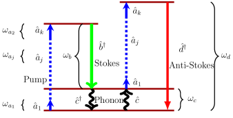
Figure 1: (Color online) The schematic energy diagram for multi-photon non-degenerate hyper-Raman processes. Here, we have shown $k$ pump $\left(a_{i}\right),$ Stokes $\left(b\right),$ vibrational (phonon) $\left(c\right),$ and anti-Stokes $\left(d\right)$ modes.

Specifically, if we choose $a_{1}=a_{2}$ (i.e., $\omega_{1}=\omega_{2}$) for $k=2$ then we would obtain the Hamiltonian of degenerate hyper-Raman process which is already studied in a reasonably detailed manner in Ref. Sen and Mandal (2007). Apart from this, 2-pump mode non-degenerate hyper-Raman process was discussed in Ref. Peřina et al. (1984). The present Hamiltonian can be viewed as a generalization of this case to multi-mode pump non-degenerate hyper-Raman process. However, nonclassical properties of multi-mode pump non-degenerate Hamiltonian is not studied in that detail. This is why we are interested in the operator solution of the Hamiltonian of non-degenerate multi-photon pump hyper-Raman process. To obtain the solution, first we write the Heisenberg’s equations of motion for different modes as

$$\begin{array}[]{lcl}\dot{a_{j}}&=&-i\omega_{j}a_{j}+\prod_{i=1:i\neq j}^{k}\left(ig^{*}a_{i}^{\dagger}bc+i\chi a_{i}^{\dagger}c^{\dagger}d\right),\\ \dot{b}&=&-i\omega_{b}b+ig\prod_{i=1}^{k}a_{i}c^{\dagger},\\ \dot{c}&=&-i\omega_{c}c+\prod_{i=1}^{k}\left(iga_{i}b^{\dagger}+i\chi a_{i}^{\dagger}d\right),\\ \dot{d}&=&-i\omega_{d}d+i\chi^{*}\prod_{i=1}^{k}a_{i}c,\end{array}$$ (2)

for which we derive the solution, using Sen-Mandal perturbative (Thapliyal et al. (2014a, b, 2016); Sen and Mandal (2005) and references therein) approach, as

$$\begin{array}[]{lcl}a_{j}(t)&=&\prod_{i=1:i\neq j}^{k}\left(f_{1_{j}}a_{j}(0)+f_{2_{j}}a_{i}^{\dagger}(0)b(0)c(0)+f_{3_{j}}a_{i}^{\dagger}(0)c^{\dagger}(0)d(0)\right.\\ &+&f_{4_{j}}a_{j}(0)A_{l}b^{\dagger}(0)b(0)c^{\dagger}(0)c(0)+f_{5_{j}}a_{i}^{\dagger}(0)a_{i}(0)a_{j}(0)b(0)b^{\dagger}(0)\\ &+&f_{6_{j}}a_{i}^{\dagger}(0)a_{i}(0)a_{j}(0)c^{\dagger}(0)c(0)+f_{7_{j}}a_{j}(0)A_{l}b(0)c^{2}(0)d^{\dagger}(0)\\ &+&f_{8_{j}}a_{j}^{\dagger}(0)a_{i}^{\dagger 2}(0)b(0)d(0)+f_{9_{j}}a_{j}(0)A_{l}b^{\dagger}(0)c^{\dagger 2}(0)d(0)\\ &+&f_{10_{j}}a_{j}(0)a_{i}^{\dagger}(0)a_{i}(0)d^{\dagger}(0)d(0)+f_{11_{j}}a_{j}(0)A_{l}c(0)c^{\dagger}(0)d^{\dagger}(0)d(0)\\ &+&\left.f_{12_{j}}a_{i}^{\dagger}(0)a_{i}(0)a_{j}(0)c^{\dagger}(0)c(0)\right),\\ b(t)&=&\prod_{i=1}^{k}\left(g_{1}b(0)+g_{2}a_{i}(0)c^{\dagger}(0)+g_{3}a_{i}^{2}(0)d^{\dagger}(0)+g_{4}a_{i}^{\dagger}(0)a_{i}(0)b(0)\right.\\ &+&\left.g_{5}A_{l}b(0)c^{\dagger}(0)c(0)+g_{6}A_{l}c^{\dagger 2}(0)d(0)\right),\\ c(t)&=&\prod_{i=1}^{k}\left(h_{1}c(0)+h_{2}a_{i}(0)b^{\dagger}(0)+h_{3}a_{i}^{\dagger}(0)d(0)+h_{4}a_{i}^{\dagger}(0)a_{i}(0)c(0)\right.\\ &+&h_{5}A_{l}b^{\dagger}(0)b(0)c(0)+h_{6}A_{l}b^{\dagger}(0)c^{\dagger}(0)d(0)+h_{7}A_{l}c(0)d^{\dagger}(0)d(0)\\ &+&\left.h_{8}a_{i}^{\dagger}(0)a_{i}(0)c(0)\right),\\ d(t)&=&\prod_{i=1}^{k}\left(l_{1}d(0)+l_{2}a_{i}(0)c(0)+l_{3}a_{i}^{2}(0)b^{\dagger}(0)+l_{4}A_{l}b(0)c^{2}(0)\right.\\ &+&\left.l_{5}A_{l}c^{\dagger}(0)c(0)d(0)+l_{6}a_{i}(0)a_{i}^{\dagger}(0)d(0)\right),\end{array}$$ (3)

where $A_{l}=\prod_{i}\left(a_{i}(0)a_{i}^{\dagger}(0)-a_{i}^{\dagger}(0)a_{i}(0)\right)$ (which gives us $l=2^{k}-1$ terms in $k$ pump mode case). For example, for 2-pump non-degenerate hyper-Raman process, we obtain $l=3$ terms as follows, $A_{3}=\left(\left\{a_{1}^{\dagger}(0)a_{1}(0)+1\right\}\left\{a_{2}^{\dagger}(0)a_{2}(0)+1\right\}\right.-\left.a_{1}^{\dagger}(0)a_{1}(0)a_{2}^{\dagger}(0)a_{2}(0)\right)=\left(a_{1}^{\dagger}(0)a_{1}(0)+a_{2}^{\dagger}(0)a_{2}(0)+1\right).$ Further, various terms in Eq. (3) are given as Eqs. (A.1)-(A.4) in Appendix A. The details of obtaining the Sen-Mandal perturbative solution are given in Appendix B. Here, it is also worth mentioning that we have neglected all the terms higher than quadratic in coupling constants $\chi$ and $g$ while obtaining the present solution.

The most general nature of the Hamiltonian describing the hyper-Raman processes used here has already been established. On top of that, the obtained solution is also quite general in nature and it is imperative to mention here that all the existing solutions of various Raman Sen and Mandal (2005); Sen et al. (2007); Sen and Mandal (2008); Sen et al. (2011) and degenerate-hyper-Raman Sen and Mandal (2007) processes can be obtained as the limiting cases of the present solution. It is also relevant to mention here that the solution obtained in Sen and Mandal (2005), which is a limiting case of the present solution, has already been shown to be reducible to the short-time solution reported till then Peřina (1991); Szlachetka et al. (1979, 1980). It is also important to note here that in some of our recent works, it has been established that the Sen-Mandal perturbative solutions are more general than the corresponding short-time solutions for the same systems (Sen and Mandal (2005); Sen et al. (2007); Sen and Mandal (2008); Sen et al. (2011); Sen and Mandal (2007); Thapliyal et al. (2014a, b, 2016) and references therein). To reduce our general solution to the solution for degenerate hyper-Raman process reported in Sen and Mandal (2007) we need to consider $k=2$, with $a_{1}=a_{2}=a$, and $\omega_{1}=\omega_{2}=\omega_{a}$ (as the process is degenerate), and $\chi$ and $g$ to be real (as $\chi$ and $g$ were considered as real in Ref. Sen and Mandal (2007)). The coupling constants $\chi$ and $g$ were treated as real in the case of Raman process, too Sen and Mandal (2005), but to be consistent with the convention used in Ref. Sen and Mandal (2005) and to reduce the solution reported here to the solution reported in Sen and Mandal (2005), we would require to replace $g$ by $-g$. Specifically, the solution used in Sen and Mandal (2005); Sen et al. (2007); Sen and Mandal (2008); Sen et al. (2011, 2013); Giri et al. (2016) can be reproduced using $k=1$, $\omega_{1}=\omega_{a}$ in the present solution. The relation among various time dependent functional coefficients in the evolution of the pump mode in the present case and previous results Sen and Mandal (2005); Sen et al. (2007); Sen and Mandal (2008); Sen et al. (2011); Sen and Mandal (2007); Sen et al. (2013); Giri et al. (2016) is summarized in Table 1. A similar correspondence among the functions for the remaining modes is mentioned explicitly in Table B.I (see Appendix B).

Multi-photon pump hyper-Raman case	Degenerate hyper-Raman case Sen and Mandal (2007)	Raman case Sen and Mandal (2005)
$f_{1_{i}}$	$f_{1}^{{}^{\prime}}$	$f_{1}^{{}^{\prime\prime}}$
$f_{2_{i}}$	$f_{2}^{{}^{\prime}}$	$f_{2}^{{}^{\prime\prime}}$
$f_{3_{i}}$	$f_{3}^{{}^{\prime}}$	$f_{3}^{{}^{\prime\prime}}$
$f_{4_{i}}$	$f_{7}^{{}^{\prime}}$
$f_{5_{i}}$	$f_{9}^{{}^{\prime}}$	$f_{5}^{{}^{\prime\prime}}$
$f_{6_{i}}$	$f_{8}^{{}^{\prime}}$	$f_{6}^{{}^{\prime\prime}}$
$f_{7_{i}}$	$f_{4}^{{}^{\prime}}$
$f_{8_{i}}$	$f_{6}^{{}^{\prime}}$	$f_{4}^{{}^{\prime\prime}}$
$f_{9_{i}}$	$f_{5}^{{}^{\prime}}$
$f_{10_{i}}$	$f_{11}^{{}^{\prime}}$	$f_{8}^{{}^{\prime\prime}}$
$f_{11_{i}}$	$f_{10}^{{}^{\prime}}$
$f_{12_{i}}$	$f_{12}^{{}^{\prime}}$	$f_{7}^{{}^{\prime\prime}}$

Table 1: The present solution is general in nature, and the existing solutions for Raman and degenerate hyper-Raman processes can be obtained as special cases of the present solution for the functions in the evolution of pump modes. Here, we have used a (two) prime(s) in the superscript of the functions $f_{i}$s to distinguish the present solution from the degenerate hyper-Raman (Raman) process.

III Criteria of nonclassicalities

Once we have the closed form analytic expressions for the evolution of various field and phonon modes involved in the process (given in Eq. (3)), we can test the nonclassical properties of the process using various moments-based criteria (such as listed in Miranowicz et al. (2010)), which are essentially the expectation values of annihilation and creation operators of the modes under consideration. Although an infinite set of moment-based criteria would be essential to form a necessary criterion of nonclassicality that would be equivalent to $P$-function Richter and Vogel (2002), here, we only use a small subset of this infinite set, which is therefore only sufficient. However, this small set of noncassicality criteria is found to be good enough to establish the highly nonclassical character of the non-degenarate hyper-Raman process. In this section, we enlist the set of criteria that is used in the present work to analyze the presence of lower and higher order nonclassicality. With the advent of sophisticated experimental techniques, some exciting experimental results involving a few of these moments-based higher order nonclassicality criteria have been reported in the recent past Allevi et al. (2012a, b); Avenhaus et al. (2010); Hamar et al. (2014). More recently, experimental detection of higher order nonclassicality up to ninth order has also been reported Peřina Jr. et al. (2017). Further, in Section I, we have already mentioned several recent applications of nonclassical states and Raman processes. Because of the above mentioned facts, in what follows, we are interested in analyzing the nonclassical properties of the process with specific attention to squeezed, antibunched and entangled states.

III.1 Lower and higher order squeezing

In order to study the squeezing effects in the various modes, we define the quadrature operators

$$\begin{array}[]{lcl}X_{a}&=&\frac{1}{2}\left(a(t)+a^{\dagger}(t)\right),\\ Y_{a}&=&-\frac{i}{2}\left(a(t)-a^{\dagger}(t)\right),\end{array}$$ (4)

where $a\,(a^{{}^{\dagger}})$ is the annihilation (creation) operator for a specific bosonic mode, and it satisfies $[a,a^{\dagger}]=1$. Squeezing in mode $a$ is possible if the fluctuation in one of the quadrature operators goes below the minimum uncertainty level, i.e., if

$$\left(\Delta X_{a}\right)^{2}<\frac{1}{4}\,\mathrm{or}\,\left(\Delta Y_{a}\right)^{2}<\frac{1}{4}.$$ (5)

Similarly, we may study intermodal squeezing in the compound mode $ab$ using the following quadrature operator for the compound mode introduced by Loudon and Knight Loudon and Knight (1987):

$$\begin{array}[]{lcl}X_{ab}&=&\frac{1}{2\sqrt{2}}\left(a(t)+a^{\dagger}(t)+b(t)+b^{\dagger}(t)\right)\\ Y_{ab}&=&-\frac{i}{2\sqrt{2}}\left(a(t)-a^{\dagger}(t)+b(t)-b^{\dagger}(t)\right).\end{array}$$ (6)

Usually, the higher order counterpart of squeezing is studied using two different criteria, proposed by Hong and Mandel Hong and Mandel (1985a, b) and Hillery Hillery (1987), independently. Hong-Mandel-type squeezing takes into consideration the higher order moments of usual quadrature defined in Eq. (4), while Hillery’s squeezing criterion deals with amplitude powered quadratures. Here, we have focused only on the latter type. For which, the amplitude powered quadratures are defined as

$$Y_{1,a}=\frac{a^{n}+\left(a^{\dagger}\right)^{n}}{2}$$ (7)

and

$$Y_{2,a}=i\left(\frac{\left(a^{\dagger}\right)^{n}-a^{n}}{2}\right).$$ (8)

As the quadratures fail to commute, we can obtain a criterion for amplitude powered squeezing from the uncertainty principle as

$$A_{i,a}=\left(\Delta Y_{i,a}\right)^{2}-\frac{1}{2}\left|\left\langle\left[Y_{1,a},Y_{2,a}\right]\right\rangle\right|<0$$ (9)

for each quadrature $i\in\left\{1,2\right\}$, where $\left[A,B\right]=AB-BA$ is the commutator, and $\left[Y_{1,a},Y_{2,a}\right]\neq 0\forall n$.

III.2 Lower and higher order antibunching

Higher order antibunching criterion was introduced by Lee Lee (1990). With time, several variants of this criterion, which are essentially equivalent, have been proposed. One such criterion was proposed by Pathak and Garcia Pathak and Garcia (2006) as

$$\begin{array}[]{lcl}D_{a}(n-1)=\left\langle a^{\dagger n}a^{n}\right\rangle-\left\langle a^{\dagger}a\right\rangle^{n}&<&0.\end{array}$$ (10)

Importantly, for $n=2$, it reduces to lower order antibunching, while for all $n\geq 3$ we obtain the higher order counterpart. Therefore, here we have calculated and reported $\left(n-1\right)$th order antibunching and also inferred corresponding lower order results from it.

Similarly, in order to study the intermodal antibunching, one can use the solution reported here and the following criterion

$$D_{ab}=(\Delta N_{ab})^{2}=\left\langle a^{\dagger}b^{\dagger}ba\right\rangle-\left\langle a^{\dagger}a\right\rangle\left\langle b^{\dagger}b\right\rangle<0.$$ (11)

III.3 Lower and higher order entanglement

Along the same line, two higher order entanglement criteria were proposed by Hillery and Zubairy Hillery and Zubairy (2006a, b) as inseparability criteria. It may be noted that each of these criteria are sufficient but not necessary and thus the entanglement (nonclassical nature) not detected by a particular criterion may be detected by the other one, and in some situations both of them may fail to detect entanglement. A quantum state can be verified to be entangled using Hillery-Zubairy’s HZ-I criterion

$$E_{ab}^{m,n}=\left\langle\left(a^{\dagger}\right)^{m}a^{m}\left(b^{\dagger}\right)^{n}b^{n}\right\rangle-\left|\left\langle a^{m}\left(b^{\dagger}\right)^{n}\right\rangle\right|^{2}<0$$ (12)

or Hillery-Zubairy’s HZ-II criterion

$$E_{ab}^{\prime m,n}=\left\langle\left(a^{\dagger}\right)^{m}a^{m}\right\rangle\left\langle\left(b^{\dagger}\right)^{n}b^{n}\right\rangle-\left|\left\langle a^{m}b^{n}\right\rangle\right|^{2}<0.$$ (13)

An arbitrary quantum state is higher order entangled if it satisfies HZ-I and/or HZ-II criteria for $m+n\geq 3$. Importantly, the lower order entanglement can also be verified from Eqs. (12) and (13), by considering $m=n=1$.

IV Nonclassicality observed

All the nonclassicality criteria listed in Eqs. (5)-(13) contain average values of functions of time evolved annihilation and creation operators given in Eq. (3). To calculate the average values, we have to consider an initial state of the system. Without any loss of generality, the initial state is chosen to be a product state of coherent states in each mode

$$|\psi(0)\rangle=|\alpha_{i}\rangle\otimes|\beta\rangle\otimes|\gamma\rangle\otimes|\delta\rangle,$$ (14)

where $|\alpha_{i}\rangle=|\alpha_{1}\rangle\otimes|\alpha_{2}\rangle\otimes\cdots|\alpha_{i}\rangle\cdots\otimes|\alpha_{k}\rangle$ is the initial state of the pump modes in the product state of $k$ coherent states.

Further, we have considered a detuning of $\left|\frac{\Delta\omega_{1}}{g}\right|=10$ and $\left|\frac{\Delta\omega_{2}}{g}\right|=19$ in Stokes and anti-Stokes hyper-Raman processes, respectively. In the stimulated case, we have considered non-zero photon number initially in each mode, i.e., $\left|\beta\right|=8,$ $\left|\gamma\right|=0.01,$ and $\left|\delta\right|=1$, while all these values are initially zero in the spontaneous case. Additionally, we have considered $\left|\alpha_{i}\right|=10$ for all the pump modes, unless stated otherwise, in both the stimulated and spontaneous cases.

IV.1 Lower and higher order squeezing

Using Eqs. (3) and (14) in criterion of squeezing (5), we have obtained the closed form analytic expressions for the witnesses of squeezing in all the modes involved. Specifically, the witnesses for the single mode squeezing in an arbitrary pump mode is calculated to be

$$\begin{array}[]{lcl}\left[\begin{array}[]{c}\left(\Delta X_{a_{j}}\right)^{2}\\ \left(\Delta Y_{a_{j}}\right)^{2}\end{array}\right]&=&\frac{1}{4}\left[1+2\left|f_{2}\right|^{2}\sigma_{l}\left|\beta\right|^{2}\left|\gamma\right|^{2}+2\left|f_{3}\right|^{2}\left|\delta\right|^{2}\right.\\ &\times&\left(\left|\alpha_{i}\right|^{2}+\sigma_{l}\left(\left|\gamma\right|^{2}+1\right)\right)+2\left\{f_{2}^{*}f_{3}\sigma_{l}\right.\\ &\times&\left.\left.\beta^{*}\gamma^{*2}\delta\mp f_{1}^{2}g_{3}^{*}g_{1}\alpha_{i}^{*2}\beta\delta+{\rm c.c.}\right\}\right],\end{array}$$ (15a)

while the witnesses of squeezing in Stokes and vibration (phonon) modes are obtained as

$$\begin{array}[]{lcl}\left[\begin{array}[]{c}\left(\Delta X_{b}\right)^{2}\\ \left(\Delta Y_{b}\right)^{2}\end{array}\right]&=&\frac{1}{4}\left[1+2\left|g_{2}\right|^{2}\left|\alpha_{i}\right|^{2}\right]\end{array}$$ (15b)

and

$$\begin{array}[]{lcl}\left[\begin{array}[]{c}\left(\Delta X_{c}\right)^{2}\\ \left(\Delta Y_{c}\right)^{2}\end{array}\right]&=&\frac{1}{4}\left[1+2\left|h_{2}\right|^{2}\left|\alpha_{i}\right|^{2}+2\left|h_{3}\right|^{2}\sigma_{l}\left|\delta\right|^{2}\right.\\ &\pm&\left.\left\{2h_{1}^{2}g_{1}^{*}g_{6}\sigma_{l}\beta^{*}\delta+{\rm c.c.}\right\}\right],\end{array}$$ (15c)

respectively. Using the obtained Sen-Mandal perturbative solution, squeezing in anti-Stokes mode was not observed, i.e.,

$$\begin{array}[]{lcl}\left[\begin{array}[]{c}\left(\Delta X_{d}\right)^{2}\\ \left(\Delta Y_{d}\right)^{2}\end{array}\right]&=&\frac{1}{4}.\end{array}$$ (15d)

Here, and in what follows we have used $\sigma_{l}=\langle A_{l}\rangle$. In Eq. (15b), we can observe a positive quantity is added to $\frac{1}{4}$, therefore, none of these quadratures can show variance less than $\frac{1}{4}$, and consequently, squeezing cannot be observed in these quadratures. However, unlike Stokes and anti-Stokes modes, the compact expressions for squeezing in all the remaining modes are complex enough to infer directly from them. To analyze the dependence of squeezing in all these modes on various parameters we performed a rigorous numerical analysis of the obtained expressions. To do so, we have used $\underset{i}{\sum}\frac{\omega_{i}}{g}=1000.0001\times 10^{5},$ $\frac{\omega_{b}}{g}=999.999\times 10^{5},$ $\frac{\omega_{c}}{g}=0.001\times 10^{5},$ and $\frac{\omega_{d}}{g}=1000.00091\times 10^{5}.$ In 2-pump mode non-degenerate hyper-Raman processes, $\frac{\omega_{1}}{g}=600.0001\times 10^{5}$ and $\frac{\omega_{2}}{g}=400\times 10^{5}$; while in 3-pump mode non-degenerate hyper-Raman processes, $\frac{\omega_{1}}{g}=100.0001\times 10^{5},$ $\frac{\omega_{2}}{g}=700\times 10^{5}$ and $\frac{\omega_{3}}{g}=200\times 10^{5}.$ Further, for the sake of simplicity, in the following discussion we have subtracted $\frac{1}{4}$ from both sides of all the expressions of squeezing. This helps us to plot the variation of squeezing parameter in a manner consistent with the remaining illustrations where the negative regions of the plots depict nonclassicality.

The study revealed that squeezing in the stimulated case of non-degenerate $k$-pump hyper-Raman process is observed only in the pump mode, which is shown to vary with various parameters. Thus, in turn, these parameters can be used to control the amount of squeezing. Specifically, witnesses of squeezing are found to be independent of the phases of different pump modes. However, the amount of squeezing is found to depend on the frequency of the pump modes. This fact can be established from Figure 2 (a)-(c), where we can observe different amount of squeezing for each mode with different frequency, which becomes the same in the degenerate case. Further, different natures of squeezing for degenerate and non-degenerate cases have been observed (cf. Figure 2 (a) and (d)). This point is also established in context of the spontaneous case in Figure 8 (d) discussed later. Additionally, the amount of squeezing in a particular pump mode can also be controlled by the intensity of one of the other pump modes (cf. Figure 2 (a) and (b)). Note that we have shown the variation in quadrature squeezing for relatively smaller time domain to establish its dependence on various independent parameters. Only due to this reason, the amount of squeezing appears to be very small (in the order of $10^{-12}$ in Figure 2 (a)). However, we observed relatively higher amount of squeezing for a larger rescaled time as shown in inset in Figure 2 (a) in case of $X_{a_{1}}$ quadrature. Similar highly oscillating nature is also observed in all other cases of single mode and intermodal squeezing, too, but being repetitive, such illustrations are not included in the subsequent plots.

Similarly, intermodal squeezing in the compound two-mode cases can be studied using Loudon and Knight’s criterion given in Eq. (6) with Eqs. (3) and (14). We are reporting here the analytic expressions of two-mode squeezing for compound pump-pump mode as

$$\begin{array}[]{lcl}\left[\begin{array}[]{c}\left(\Delta X_{a_{j}a_{r}}\right)^{2}\\ \left(\Delta Y_{a_{j}a_{r}}\right)^{2}\end{array}\right]&=&\frac{1}{4}\left[2\left(\left[\begin{array}[]{c}\left(\Delta X_{a_{j}}\right)^{2}\\ \left(\Delta Y_{a_{j}}\right)^{2}\end{array}\right]+\left[\begin{array}[]{c}\left(\Delta X_{a_{r}}\right)^{2}\\ \left(\Delta Y_{a_{r}}\right)^{2}\end{array}\right]\right)+\left\{f_{2}r_{2}^{*}\left|\beta\right|^{2}\left|\gamma\right|^{2}\alpha_{j}\alpha_{r}^{*}\sigma_{l}+f_{3}r_{2}^{*}\alpha_{j}\alpha_{r}^{*}\sigma_{l}\beta^{*}\gamma^{*2}\delta\right.\right.\\ &+&f_{2}r_{3}^{*}\alpha_{j}\alpha_{r}^{*}\sigma_{l}\beta\gamma^{2}\delta^{*}\pm\left\{f_{1}r_{2}\alpha_{i}^{*}\beta\gamma+f_{1}r_{3}\alpha_{i}^{*}\beta^{*}\delta+f_{1}r_{4}\left|\beta\right|^{2}\left|\gamma\right|^{2}\alpha_{j}\alpha_{r}\sigma_{l}+f_{1}r_{5}\left|\alpha_{i}\right|^{2}\left(\left|\beta\right|^{2}+1\right)\alpha_{j}\alpha_{r}\right.\\ &+&\left(f_{1}r_{6}+f_{1}r_{12}\right)\left|\alpha_{i}\right|^{2}\left|\gamma\right|^{2}\alpha_{j}\alpha_{r}+f_{1}r_{10}\left(\left|\alpha_{i}\right|^{2}+\sigma_{l}\left(\left|\gamma\right|^{2}+1\right)\right)\left|\delta\right|^{2}\alpha_{j}\alpha_{r}+f_{1}r_{7}\alpha_{j}\alpha_{r}\sigma_{l}\beta\gamma^{2}\delta^{*}\\ &+&\left.\left.\left.\left(2f_{1}r_{8}+f_{2}r_{3}\right)\alpha_{j}^{*}\alpha_{r}^{*}\alpha_{i}^{*2}\beta\delta+f_{1}r_{9}\alpha_{j}\alpha_{r}\sigma_{l}\beta^{*}\gamma^{*2}\delta\right\}+f_{3}r_{3}^{*}\left(\left|\alpha_{i}\right|^{2}+\sigma_{l}\left(\left|\gamma\right|^{2}+1\right)\right)\left|\delta\right|^{2}\alpha_{j}\alpha_{r}^{*}+{\rm c.c.}\right\}\right],\end{array}$$ (16a)

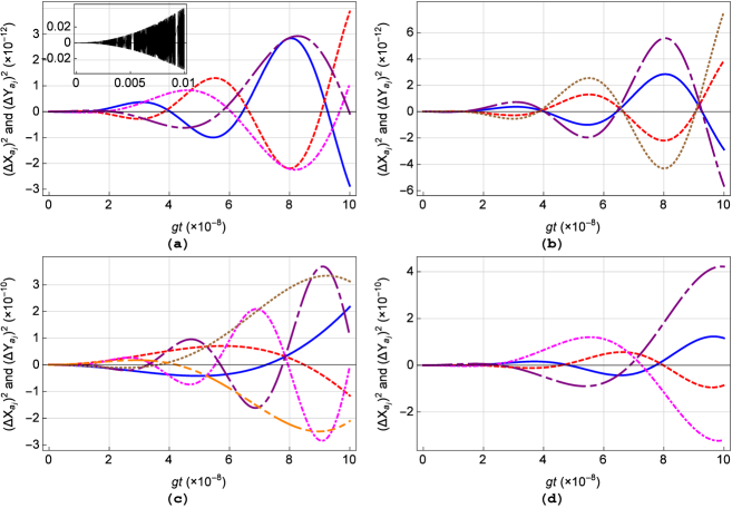
Figure 2: (Color online) Squeezing in $j$th pump mode. Squeezing in both modes of the 2-pump modes non-degenerate stimulated hyper-Raman processes with (a) $\left|\alpha_{1}\right|=\left|\alpha_{2}\right|=10$, and (b) $\left|\alpha_{1}\right|=10,$ $\left|\alpha_{2}\right|=12$. (c) Squeezing in all three modes of the 3-pump modes non-degenerate hyper-Raman processes with $\left|\alpha_{1}\right|=\left|\alpha_{2}\right|=\left|\alpha_{3}\right|=10$. (d) Squeezing in degenerate hyper-Raman processes for the cases with 2 and 3-pump modes is compared. Here, we have amplified the variation in the case of 2-pump modes 30 times to show it with the squeezing in 3-pump modes. In all the cases, the solid-blue, dot-dashed-magenta, and dotted-black lines represent the quadrature $\left(\Delta X_{a_{j}}\right)^{2}$; and dashed-red, purple-large-dot-dashed, and orange-double-dotted-dashed lines correspond to the quadrature $\left(\Delta Y_{a_{j}}\right)^{2}$.

which is applicable to any arbitrary pump modes $a_{j}$ and $a_{r}$. Compound pump-Stokes, pump-vibration, and pump-anti-Stokes modes squeezing are obtained as

$$\begin{array}[]{lcl}\left[\begin{array}[]{c}\left(\Delta X_{a_{j}b}\right)^{2}\\ \left(\Delta Y_{a_{j}b}\right)^{2}\end{array}\right]&=&\frac{1}{4}\left[2\left(\left[\begin{array}[]{c}\left(\Delta X_{a_{j}}\right)^{2}\\ \left(\Delta Y_{a_{j}}\right)^{2}\end{array}\right]+\left[\begin{array}[]{c}\left(\Delta X_{b}\right)^{2}\\ \left(\Delta Y_{b}\right)^{2}\end{array}\right]\right)+\left\{f_{3}g_{2}^{*}\alpha_{j}^{*}\alpha_{i}^{*2}\delta\mp f_{4}g_{1}\left|\alpha_{i}\right|^{2}\alpha_{j}\beta\mp f_{1}g_{4}\left|\gamma\right|^{2}\sigma_{l}\alpha_{j}\beta\right.\right.\\ &\pm&\left.\left.f_{1}g_{6}\sigma_{l}\alpha_{j}\gamma^{*2}\delta+{\rm c.c.}\right\}\right],\end{array}$$ (16b)

$$\begin{array}[]{lcl}\left[\begin{array}[]{c}\left(\Delta X_{a_{j}c}\right)^{2}\\ \left(\Delta Y_{a_{j}c}\right)^{2}\end{array}\right]&=&\frac{1}{4}\left[2\left(\left[\begin{array}[]{c}\left(\Delta X_{a_{j}}\right)^{2}\\ \left(\Delta Y_{a_{j}}\right)^{2}\end{array}\right]+\left[\begin{array}[]{c}\left(\Delta X_{c}\right)^{2}\\ \left(\Delta Y_{c}\right)^{2}\end{array}\right]\right)+\left\{f_{2}h_{3}^{*}\sigma_{l}\alpha_{j}\beta\gamma\delta^{*}+f_{3}h_{3}^{*}\left|\delta\right|^{2}\sigma_{l}\alpha_{j}\gamma^{*}\pm\left(f_{1}h_{7}-f_{4}h_{1}\right)\left|\alpha_{i}\right|^{2}\alpha_{j}\gamma\right.\right.\\ &\pm&\left.\left.f_{1}h_{3}\alpha_{i}^{*}\delta\pm f_{1}h_{4}\left|\beta\right|^{2}\sigma_{l}\alpha_{j}\gamma\pm f_{1}h_{6}\sigma_{l}\alpha_{j}\beta^{*}\gamma^{*}\delta\pm f_{1}h_{7}\left|\delta\right|^{2}\sigma_{l}\alpha_{j}\gamma+{\rm c.c.}\right\}\right],\end{array}$$ (16c)

and

$$\begin{array}[]{lcl}\left[\begin{array}[]{c}\left(\Delta X_{a_{j}d}\right)^{2}\\ \left(\Delta Y_{a_{j}d}\right)^{2}\end{array}\right]&=&\frac{1}{4}\left[2\left(\frac{1}{2}+\left[\begin{array}[]{c}\left(\Delta X_{a_{j}}\right)^{2}\\ \left(\Delta Y_{a_{j}}\right)^{2}\end{array}\right]\right)+\left\{f_{1}l_{4}\sigma_{l}\alpha_{j}\beta\gamma^{2}\pm f_{1}l_{5}\alpha_{j}\delta\left(\left|\alpha_{i}\right|^{2}+\sigma_{l}\left(\left|\gamma\right|^{2}+1\right)\right)+{\rm c.c.}\right\}\right],\end{array}$$ (16d)

respectively. We have also considered two-mode squeezing among Stokes-vibration mode

$$\begin{array}[]{lcl}\left[\begin{array}[]{c}\left(\Delta X_{bc}\right)^{2}\\ \left(\Delta Y_{bc}\right)^{2}\end{array}\right]&=&\frac{1}{4}\left[2\left(\left[\begin{array}[]{c}\left(\Delta X_{b}\right)^{2}\\ \left(\Delta Y_{b}\right)^{2}\end{array}\right]+\left[\begin{array}[]{c}\left(\Delta X_{c}\right)^{2}\\ \left(\Delta Y_{c}\right)^{2}\end{array}\right]\right)+\left\{g_{2}h_{2}^{*}\sigma_{l}\beta\gamma^{*}\pm\left(g_{1}h_{2}\alpha_{i}+g_{1}h_{5}\sigma_{l}\beta\gamma+2g_{6}h_{1}\sigma_{l}\gamma^{*}\delta\right)+{\rm c.c.}\right\}\right],\end{array}$$ (16e)

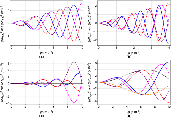
Figure 3: (Color online) Intermodal squeezing is observed in 2-pump modes non-degenerate stimulated hyper-Raman processes in (a) $j$th pump-Stokes mode, (b) $j$th pump-vibration mode, and (c) $j$th pump-anti-Stokes mode. In all three cases, the solid-blue (dot-dashed-magenta) and dashed-red (purple-large-dot-dashed) lines correspond to the quadratures $\left(\Delta X_{a_{j}K}\right)^{2}$ and $\left(\Delta Y_{a_{j}K}\right)^{2}$ for compound $a_{1}K$ ($a_{2}K$) mode, respectively. While in (d), intermodal squeezing in compound $a_{j}a_{k}$ mode for 3-pump modes non-degenerate stimulated hyper-Raman processes is shown for all three cases, i.e., $a_{1}a_{2}$ mode shown in solid-blue and dashed-red lines, $a_{2}a_{3}$ mode shown in dot-dashed-magenta and purple-large-dot-dashed lines, and $a_{1}a_{3}$ mode as dotted-black and orange-double-dotted-dashed lines for the quadratures $\left(\Delta X_{a_{j}a_{r}}\right)^{2}$ and $\left(\Delta Y_{a_{j}a_{r}}\right)^{2}$, respectively. In all the cases, $\left|\alpha_{i}\right|=10\,\forall i\in\left\{1,2,3\right\}$.

Stokes-anti-Stokes mode

$$\begin{array}[]{lcl}\left[\begin{array}[]{c}\left(\Delta X_{bd}\right)^{2}\\ \left(\Delta Y_{bd}\right)^{2}\end{array}\right]&=&\frac{1}{4}\left[1+\frac{1}{2}\left[\begin{array}[]{c}\left(\Delta X_{b}\right)^{2}\\ \left(\Delta Y_{b}\right)^{2}\end{array}\right]\pm\left\{g_{1}l_{3}\alpha_{i}^{2}+{\rm c.c.}\right\}\right],\end{array}$$ (16f)

and vibration-anti-Stokes mode

$$\begin{array}[]{lcl}\left[\begin{array}[]{c}\left(\Delta X_{cd}\right)^{2}\\ \left(\Delta Y_{cd}\right)^{2}\end{array}\right]&=&\frac{1}{4}\left[1+\frac{1}{2}\left[\begin{array}[]{c}\left(\Delta X_{c}\right)^{2}\\ \left(\Delta Y_{c}\right)^{2}\end{array}\right]\pm\left\{h_{1}l_{5}\sigma_{l}\gamma\delta+{\rm c.c.}\right\}\right].\end{array}$$ (16g)

In all the expressions obtained for two-mode squeezing (i.e., Eqs. (16a)-(16g)), the single mode squeezing witnesses (i.e., variance $\left(\Delta X_{i}\right)^{2}$, and $\left(\Delta Y_{i}\right)^{2}$, with $i\in{a,b,c}$) that appear in the right hand sides are to be substituted by the corresponding expressions reported for single mode squeezing in Eqs. (15a)-(15d).

Finally, we analyzed the expressions for the compound mode squeezing, and variation is shown in Figure 3. Interestingly, intermodal squeezing is observed in all the compound modes involving pump mode. In the analogy of quadrature squeezing illustrated in Figure 2, the observed nonclassicality is shown to depend on the frequency of the pump mode. The same fact has been established here using non-degenerate 2-pump and 3-pump hyper-Raman processes, where the amount of intermodal squeezing are found to be different for various pump modes.

Hillary’s amplitude powered squeezing for all the modes involved is calculated using Eqs. (3) and (14) in criterion of squeezing (9). Specifically, the analytic expression for an arbitrary pump mode is obtained as follows

$$\begin{array}[]{lcl}\left[\begin{array}[]{c}A_{1,a_{j}}\\ A_{2,a_{j}}\end{array}\right]&=&\frac{1}{2}k^{2}\left|\alpha_{j}\right|^{2\left(k-1\right)}\left[\left|f_{2}\right|^{2}\sigma_{l}\left|\beta\right|^{2}\left|\gamma\right|^{2}\right.\\ &+&\left|f_{3}\right|^{2}\left|\delta\right|^{2}\left(\left|\alpha_{i}\right|^{2}+\sigma_{l}\left(\left|\gamma\right|^{2}+1\right)\right)\\ &+&\left.\left\{f_{2}^{*}f_{3}\sigma_{l}\beta^{*}\gamma^{*2}\delta\mp f_{1}^{2}g_{3}^{*}g_{1}\alpha_{i}^{*2}\beta\delta+{\rm c.c.}\right\}\right].\end{array}$$ (17a)

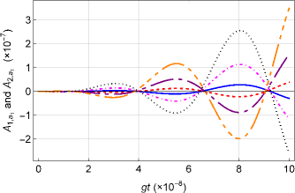
Figure 4: (Color online) Amplitude powered squeezing is observed in $a_{1}$ pump mode in 2-pump modes non-degenerate hyper-Raman processes with $\left|\alpha_{1}\right|=\left|\alpha_{2}\right|=10$. The solid-blue and dashed-red lines, dot-dashed-magenta and purple-large-dot-dashed lines, and dotted-black and orange-double-dotted-dashed lines correspond to the amplitude powered quadratures $A_{1,a_{1}}$ and $A_{1,a_{2}}$ for $k=1,2,$ and 3, respectively. To accommodate all the variations in the same plot we have amplified the values for $k=1$ and 2 with $10^{4}$ and $10^{2}$, respectively.

Similar study for Stokes, vibration, and anti-Stokes modes resulted in

$$\begin{array}[]{lcl}\left[\begin{array}[]{c}A_{1,b}\\ A_{2,b}\end{array}\right]&=&\frac{1}{2}\left[k^{2}\left|g_{2}\right|^{2}\left|\alpha_{i}\right|^{2}\left|\beta\right|^{2\left(k-1\right)}\right],\end{array}$$ (17b)

$$\begin{array}[]{lcl}\left[\begin{array}[]{c}A_{1,c}\\ A_{2,c}\end{array}\right]&=&\frac{1}{2}k^{2}\left|\gamma\right|^{2\left(k-1\right)}\left[\left(\left|h_{2}\right|^{2}\left|\alpha_{i}\right|^{2}+\left|h_{3}\right|^{2}\sigma_{l}\left|\delta\right|^{2}\right)\right.\\ &\pm&\left.\left\{h_{1}^{2k}g_{1}^{*}g_{6}\sigma_{l}\beta^{*}\delta+{\rm c.c.}\right\}\right],\end{array}$$ (17c)

and

$$\begin{array}[]{lcl}\left[\begin{array}[]{c}A_{1,d}\\ A_{2,d}\end{array}\right]&=&0,\end{array}$$ (17d)

respectively. From the obtained expressions, the presence of amplitude powered squeezing in the pump mode has been observed. Similar to the quadrature squeezing (shown in Figure 2), the nonclassicality is found to be absent in the remaining modes. Further, with increase in higher orders of squeezing, depth of the witness of amplitude powered squeezing is also observed to increase, which is in accordance with some of our recent observations (Thapliyal et al. (2014a, b); Giri et al. (2017) and references therein).

IV.2 Lower and higher order antibunching

Higher order antibunching criterion given in Eq. (10), used with Eqs. (3) and (14) leads to the closed analytic expressions for the pump, Stokes, vibration and anti-Stokes modes as

$$\begin{array}[]{lcl}D_{a_{j}}(n-1)&=&n\left(n-1\right)\left[\left|\alpha_{j}\right|^{2\left(n-1\right)}\left(\left|f_{2}\right|^{2}\left|\beta\right|^{2}\left|\gamma\right|^{2}\sigma_{l}\right.\right.\\ &+&\left.\left|f_{3}\right|^{2}\left|\delta\right|^{2}\left\{\left|\alpha_{i}\right|^{2}+\sigma_{l}\left(\left|\gamma\right|^{2}+1\right)\right\}\right)\\ &+&\left|\alpha_{j}\right|^{2\left(n-2\right)}\left\{f_{2}^{*}f_{3}\sigma_{l}\beta^{*}\gamma^{*2}\delta\right.\\ &-&\left.\left.g_{1}^{*}g_{3}\alpha_{j}^{2}\alpha_{i}^{2}\beta^{*}\delta^{*}+{\rm c.c.}\right\}\right],\end{array}$$ (18a)

$$\begin{array}[]{lcl}D_{b}(n-1)&=&n\left(n-1\right)\left|g_{2}\right|^{2}\left|\alpha_{i}\right|^{2}\left|\beta\right|^{2\left(n-1\right)},\end{array}$$ (18b)

$$\begin{array}[]{lcl}D_{c}(n-1)&=&n\left(n-1\right)\left[\left(\left|h_{2}\right|^{2}\left|\alpha_{i}\right|^{2}+\left|h_{3}\right|^{2}\sigma_{l}\left|\delta\right|^{2}\right)\right.\\ &\times&\left|\gamma\right|^{2\left(n-1\right)}+\left\{g_{6}^{*}g_{1}\left|\gamma\right|^{2\left(n-2\right)}\sigma_{l}\beta\gamma^{2}\delta^{*}\right.\\ &+&\left.\left.{\rm c.c.}\right\}\right],\end{array}$$ (18c)

and

$$D_{d}(n)=0,$$ (18d)

respectively.

Using these expressions we have analyzed the possibilities of observing both lower and higher order antibunching in all the modes except anti-Stokes mode (as $D_{d}(n)$ is always zero). The presence of lower and higher order antibunching in the pump mode has been observed and shown in Figure 5 (a). Antibunching is not observed in the other modes, i.e., in the modes other than the pump modes. It is also important to note here that the second-order correlation computed here for obtaining the signature of antibunching depends on the number of photons in certain mode while it is independent of its frequency.

Similarly, intermodal antibunching defined in Eq. (11) can be calculated for all the possible two-mode cases, i.e., pump-pump mode

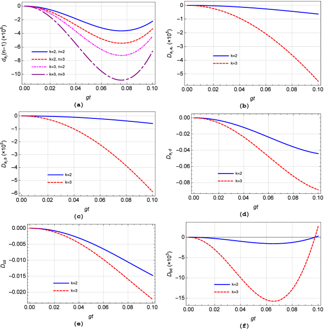
Figure 5: (Color online) Higher order antibunching and intermodal antibunching in $k$-pump modes non-degenerate hyper-Raman processes with (a) The values for lower order antibunching ($n=2$) in 2-pump (3-pump) modes non-degenerate hyper-Raman processes is multiplied by $10^{4}$ ($2\times 10^{2}$) and higher order antibunching in 2-pump modes non-degenerate hyper-Raman processes is amplified 50 times. Intermodal antibunching in (b) pump-pump, (c) pump-Stokes, (d) pump-anti-Stokes, (e) vibration-anti-Stokes, and (f) Stokes-anti-Stokes modes for 2-pump and 3-pump modes non-degenerate hyper-Raman processes. The variation in case of 2-pump modes is amplified 10 times in (b), (c), and (f), while 100 times in (d) and (e). In all the cases, we have used $\left|\alpha_{i}\right|=10$.

$$\begin{array}[]{lcl}D_{a_{j}a_{r}}&=&\left|\alpha_{j}\right|^{2}\left|\alpha_{r}\right|^{2}\left|\alpha_{i}\right|^{2}\left\{-\left|f_{2}\right|^{2}\left(\left|\beta\right|^{2}+\left|\gamma\right|^{2}+1\right)\right.+\left.\left|f_{3}\right|^{2}\left(3\left|\delta\right|^{2}-\left|\gamma\right|^{2}\right)\right\}+3\left|\alpha_{j}\right|^{2}\left|\alpha_{r}\right|^{2}\sigma_{l}\left\{\left|f_{2}\right|^{2}\right.\\ &\times&\left|\beta\right|^{2}\left|\gamma\right|^{2}+\left|f_{3}\right|^{2}\left|\delta\right|^{2}\left(\left|\gamma\right|^{2}+1\right)+\left.\left(f_{2}^{*}f_{3}\beta^{*}\gamma^{*2}\delta+{\rm c.c.}\right)\right\}+2\left(\left|\alpha_{i}\right|^{2}+\sigma_{l}\right)\\ &+&\left(\left|\alpha_{j}\right|^{2}+\left|\alpha_{r}\right|^{2}+1\right)\left\{\left|f_{2}\right|^{2}\left|\beta\right|^{2}\left|\gamma\right|^{2}\right.+\left.\left|f_{3}\right|^{2}\left|\delta\right|^{2}\left(\left|\gamma\right|^{2}+1\right)+\left(f_{2}^{*}f_{3}\beta^{*}\gamma^{*2}\delta+{\rm c.c.}\right)\right\}\\ &+&2\left|\alpha_{j}\right|^{2}\left(\left|\alpha_{i}\right|^{2}+\sigma_{l}\right)\left\{\left|f_{2}\right|^{2}\left|\beta\right|^{2}\left|\gamma\right|^{2}+\left|f_{3}\right|^{2}\left|\delta\right|^{2}\right.\left.\left(\left|\gamma\right|^{2}+1\right)+\left(f_{2}^{*}f_{3}\beta^{*}\gamma^{*2}\delta+{\rm c.c.}\right)\right\}+\left\{f_{1}^{*}f_{2}\right.\\ &\times&\alpha_{j}^{*}\alpha_{r}^{*}\alpha_{i}^{*}\beta\gamma+\left(2f_{1}^{*}f_{8}+f_{1}^{*2}f_{2}f_{3}\right)\left.\alpha_{j}^{*2}\alpha_{r}^{*2}\alpha_{i}^{*2}\beta\delta+f_{1}^{*}f_{3}\alpha_{j}^{*}\alpha_{r}^{*}\alpha_{i}^{*}\gamma^{*}\delta+{\rm c.c.}\right\},\end{array}$$ (19a)

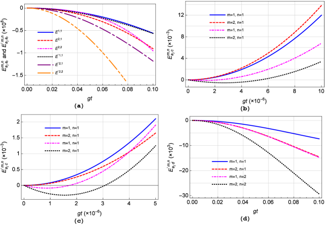
Figure 6: (Color online) The presence of lower and higher order entanglement in two pump modes is shown in (a) using HZ1 and HZ2 criteria. In (b) and (c), both lower and higher order entanglement between pump and vibration modes is established using HZ1 and HZ2 criteria, respectively. The lower order entanglement in (a) is amplified $10^{4}$ times, while higher order entanglement with $m=2,\,n=1$ (which is same as for $m=1,\,n=2$) is amplified $10^{2}$ times. The dot-dashed-magenta and dotted-black lines in (b) and (c) correspond to the phase angle $\phi_{1}=\frac{\pi}{2}$ and $-\frac{\pi}{2}$, respectively, in $\alpha_{1}=\left|\alpha_{1}\right|\exp\left(i\phi_{1}\right)$. In (b) and (c), the lower order entanglement is amplified 100 times, whereas in (d), the lower order entanglement and higher order entanglement with $m=1,\,n=2$ are amplified by 100 times, respectively. In all the cases, $\left|\alpha_{i}\right|=10$ has been used.

pump-Stokes mode

$$\begin{array}[]{lcl}D_{a_{j}b}&=&-\left|f_{2}\right|^{2}\left|\alpha_{j}\right|^{2}\left|\beta\right|^{2}\left(\left|\alpha_{i}\right|^{2}+\sigma_{l}\left|\gamma\right|^{2}\right)\\ &+&\left\{\left(f_{1}^{*}f_{9}+g_{1}^{*}g_{2}f_{1}^{*}f_{3}\right)\left|\alpha_{j}\right|^{2}\sigma_{l}\beta^{*}\gamma^{*2}\delta+{\rm c.c.}\right\},\end{array}$$ (19b)

pump-vibration mode

$$\begin{array}[]{lcl}D_{a_{j}c}&=&-\left|\alpha_{j}\right|^{2}\left|\gamma\right|^{2}\left\{\left|f_{2}\right|^{2}\left(\left|\alpha_{i}\right|^{2}+\sigma_{l}\left|\beta\right|^{2}\right)-\left|f_{3}\right|^{2}\right.\\ &\times&\left.\left(\left|\alpha_{i}\right|^{2}+\sigma_{l}\left|\delta\right|^{2}\right)\right\}+\left|f_{3}\right|^{2}\left|\delta\right|^{2}\left(\left|\alpha_{i}\right|^{2}+\sigma_{l}\right)\\ &\times&\left(2\left|\gamma\right|^{2}+1\right)+\left\{f_{1}^{*}f_{3}\alpha_{j}^{*}\alpha_{i}^{*}\gamma^{*}\delta\right.\\ &+&h_{2}^{*}h_{1}f_{1}^{*}f_{3}\alpha_{j}^{*2}\alpha_{i}^{*2}\beta\delta+f_{2}^{*}f_{3}\left(\left|\alpha_{i}\right|^{2}+\sigma_{l}\right)\beta^{*}\gamma^{*2}\delta\\ &+&\left.\left(2f_{1}^{*}f_{9}+h_{1}^{*}h_{2}f_{1}^{*}f_{3}\right)\left|\alpha_{j}\right|^{2}\sigma_{l}\beta^{*}\gamma^{*2}\delta+{\rm c.c.}\right\},\end{array}$$ (19c)

pump-anti-Stokes mode

$$\begin{array}[]{lcl}D_{a_{j}d}&=&\left|f_{3}\right|^{2}\left|\alpha_{j}\right|^{2}\left|\delta\right|^{2}\left\{\left|\alpha_{i}\right|^{2}+\sigma_{l}\left(\left|\gamma\right|^{2}+\left(\left|\delta\right|^{2}-1\right)\right)\right\}\\ &+&\left\{\left(f_{1}^{*}f_{7}+l_{1}^{*}l_{2}f_{1}^{*}f_{2}\right)\left|\alpha_{j}\right|^{2}\sigma_{l}\beta\gamma^{2}\delta^{*}+{\rm c.c.}\right\},\end{array}$$ (19d)

Stokes-vibration mode

$$\begin{array}[]{lcl}D_{bc}&=&\left|g_{2}\right|^{2}\left|\alpha_{i}\right|^{2}\left(2\left|\gamma\right|^{2}+1\right)+\left\{g_{1}^{*}g_{2}\alpha_{i}\beta^{*}\gamma^{*}\right.\\ &+&g_{1}^{*}g_{5}\left|\beta\right|^{2}\left|\gamma\right|^{2}\sigma_{l}+g_{1}^{*}g_{6}\sigma_{l}\beta^{*}\gamma^{*2}\delta\\ &+&\left.h_{2}^{*}h_{1}g_{1}^{*}g_{2}\left|\alpha_{i}\right|^{2}\left|\beta\right|^{2}+h_{3}^{*}h_{1}g_{1}^{*}g_{2}\alpha_{i}^{2}\beta^{*}\delta^{*}+{\rm c.c.}\right\},\end{array}$$ (19e)

Stokes-anti-Stokes mode

$$\begin{array}[]{lcl}D_{bd}&=&\left\{l_{1}^{*}l_{3}\alpha_{i}^{2}\beta^{*}\delta^{*}+{\rm c.c.}\right\},\end{array}$$ (19f)

and vibration-anti-Stokes mode

$$\begin{array}[]{lcc}D_{cd}&=&-\left|l_{2}\right|^{2}\left|\gamma\right|^{2}\left|\delta\right|^{2}\sigma_{l}.\end{array}$$ (19g)

From the obtained expressions, the presence of intermodal antibunching in various compound modes is shown in Figure 5. We could detect antibunching in all possible compound modes except pump-vibration and Stokes-vibration modes. It is interesting to observe that the depth of nonclassicality witness increases with the increase in number of pump modes in hyper-Raman process for the same values of the coupling constants. On top of that, two arbitrary pump modes are also found to possess intermodal antibunching as shown in Figure 5 (b).

IV.3 Lower and higher order entanglement

Inseparability of various modes can be analyzed using HZ-I and HZ-II criteria of entanglement given in Eqs. (12) and (13). For the two arbitrary pump modes the compact expression is obtained as follows

$$\begin{array}[]{lcl}\left(\begin{array}[]{c}E_{a_{j},a_{r}}^{m,n}\\ E_{a_{j},a_{r}}^{\prime m,n}\end{array}\right)&=&\left|f_{2}\right|^{2}\left|\alpha_{j}\right|^{2\left(m-1\right)}\left|\alpha_{r}\right|^{2\left(n-1\right)}\left[\left|\alpha_{i}\right|^{2}\left\{-mn\left|\alpha_{j}\right|^{2}\left|\alpha_{r}\right|^{2}\left(1+\left|\beta\right|^{2}+\left|\gamma\right|^{2}\right)\pm\left|\beta\right|^{2}\left|\gamma\right|^{2}\right.\right.\\ &\times&\left.\left(m^{2}n^{2}+m^{2}\left(2n\pm 1\right)\left|\alpha_{r}\right|^{2}+n^{2}\left(2m\pm 1\right)\left|\alpha_{j}\right|^{2}\right)\right\}+\left\{m^{2}\left(1+\left|\alpha_{r}\right|^{2}\right)\left|\alpha_{r}\right|^{2}+n^{2}\left(1+\left|\alpha_{j}\right|^{2}\right)\left|\alpha_{j}\right|^{2}\right.\\ &\pm&\left.\left.mn\left|\alpha_{j}\right|^{2}\left|\alpha_{r}\right|^{2}\right\}\sigma_{l}\left|\beta\right|^{2}\left|\gamma\right|^{2}\right]+\left|f_{3}\right|^{2}\left|\alpha_{j}\right|^{2\left(m-1\right)}\left|\alpha_{r}\right|^{2\left(n-1\right)}\left[\left|\alpha_{i}\right|^{2}\left\{\left|\delta\right|^{2}\left(m^{2}\left(1+\left|\alpha_{r}\right|^{2}\right)\left|\alpha_{r}\right|^{2}\right.\right.\right.\\ &+&\left.n^{2}\left(1+\left|\alpha_{j}\right|^{2}\right)\left|\alpha_{j}\right|^{2}+\left(m^{2}\left(1\pm 2n\right)\left|\alpha_{r}\right|^{2}+n^{2}\left(1\pm 2m\right)\left|\alpha_{j}\right|^{2}\pm m^{2}n^{2}\right)\left|\gamma\right|^{2}\right)\pm mn\left|\alpha_{j}\right|^{2}\left|\alpha_{r}\right|^{2}\\ &\times&\left.\left(\left|\delta\right|^{2}-\left|\gamma\right|^{2}\right)\right\}+\sigma_{l}\left(\left|\gamma\right|^{2}+1\right)\left|\delta\right|^{2}\left\{m^{2}\left|\alpha_{r}\right|^{2}\left(1+\left|\alpha_{r}\right|^{2}\right)+n^{2}\left(1+\left|\alpha_{j}\right|^{2}\right)\left|\alpha_{j}\right|^{2}\pm mn\left|\alpha_{j}\right|^{2}\right.\\ &\times&\left.\left.\left|\alpha_{r}\right|^{2}\right\}\right]+F_{a\pm}\pm mn\left|\alpha_{j}\right|^{2\left(m-2\right)}\left|\alpha_{r}\right|^{2\left(n-2\right)}\left[f_{2}^{*}f_{1}\alpha_{j}\alpha_{r}\alpha_{i}\beta^{*}\gamma^{*}+f_{3}^{*}f_{1}\alpha_{j}\alpha_{r}\alpha_{i}\gamma\delta^{*}+\left(f_{2}^{*2}f_{1}^{2}\right.\right.\\ &\times&\left.\alpha_{j}^{2}\alpha_{r}^{2}\alpha_{i}^{2}\beta^{*2}\gamma^{*2}+f_{3}^{*2}f_{1}^{2}\alpha_{j}^{2}\alpha_{r}^{2}\alpha_{i}^{2}\gamma^{2}\delta^{*2}\right)\left(\left(m-1\right)\left|\alpha_{r}\right|^{2}+\left(n-1\right)\left|\alpha_{j}\right|^{2}+\frac{\left(m-1\right)\left(n-1\right)}{2}\right)\\ &+&\alpha_{j}^{2}\alpha_{r}^{2}\alpha_{i}^{2}\beta^{*}\delta^{*}\left\{f_{8}^{*}f_{1}\left(\left(2\left|\alpha_{j}\right|^{2}+m-1\right)\left|\alpha_{r}\right|^{2}+\left(n-1\right)\left(\left|\alpha_{j}\right|^{2}+\frac{m-1}{2}\right)\right)+f_{1}^{2}f_{2}^{*}f_{3}^{*}\left(\left|\gamma\right|^{2}\left(n-1\right)\right.\right.\\ &\times&\left.\left.\left(2\left|\alpha_{j}\right|^{2}+m-1\right)+\left(n-1\right)\left(\left|\alpha_{j}\right|^{2}+\frac{\left(m-1\right)}{2}\right)+2\left(m-1\right)\left|\alpha_{r}\right|^{2}\left(2\left|\gamma\right|^{2}+1\right)+\left|\alpha_{r}\right|^{2}\left|\gamma\right|^{2}\right)\right\}\\ &+&f_{2}^{*}f_{3}\left|\alpha_{j}\right|^{2}\left|\alpha_{r}\right|^{2}\beta^{*}\gamma^{*2}\delta\left\{\left|\alpha_{i}\right|^{2}\left(n^{2}\left(1\pm 2m\right)\left|\alpha_{j}\right|^{2}+m^{2}\left(1\pm 2n\right)\left|\alpha_{r}\right|^{2}\pm m^{2}n^{2}\right)\right.\\ &+&\left.\left.\left.\sigma_{l}\left(n^{2}\left(1+\left|\alpha_{j}\right|^{2}\right)\left|\alpha_{j}\right|^{2}\right.+m^{2}\left(1+\left|\alpha_{r}\right|^{2}\right)\left|\alpha_{r}\right|^{2}\pm mn\left|\alpha_{j}\right|^{2}\left|\alpha_{r}\right|^{2}\right)\right\}+{\rm c.c.}\right],\end{array}$$ (20a)

where

$$\begin{array}[]{lcl}F_{a+}&=&mn\left|\alpha_{j}\right|^{2\left(m-1\right)}\left|\alpha_{r}\right|^{2\left(n-1\right)}\left(2n\left|\alpha_{j}\right|^{2}+2m\left|\alpha_{r}\right|^{2}\right.\\ &+&\left.mn\right)\left\{\left|f_{2}\right|^{2}\sigma_{l}+\left|f_{3}\right|^{2}\left|\delta\right|^{2}\left(\left|\alpha_{i}\right|^{2}+\sigma_{l}\left(\left|\gamma\right|^{2}+1\right)\right)\right.\\ &+&\left.\left(f_{2}^{*}f_{3}\sigma_{l}\beta^{*}\gamma^{*2}\delta+{\rm c.c.}\right)\right\}\end{array}$$

and $F_{a-}=0$. While the analytic expression of HZ-I and HZ-II for pump-Stokes mode is obtained as

$$\begin{array}[]{lcl}\left(\begin{array}[]{c}E_{a_{j},b}^{m,n}\\ E_{a_{j},b}^{\prime m,n}\end{array}\right)&=&\left|f_{2}\right|^{2}\left|\alpha_{j}\right|^{2\left(m-1\right)}\left|\beta\right|^{2\left(n-1\right)}\left(n\left|\alpha_{j}\right|^{2}\mp m\left|\beta\right|^{2}\right)\\ &\times&\left(n\left|\alpha_{j}\right|^{2}\left|\alpha_{i}\right|^{2}-m\sigma_{l}\left|\beta\right|^{2}\left|\gamma\right|^{2}\right)+m^{2}\left|f_{3}\right|^{2}\\ &\times&\left|\alpha_{j}\right|^{2\left(m-1\right)}\left|\beta\right|^{2n}\left|\delta\right|^{2}\left(\left|\alpha_{i}\right|^{2}+\sigma_{l}\left(\left|\gamma\right|^{2}+1\right)\right)\\ &+&m\left|\alpha_{j}\right|^{2\left(m-1\right)}\left|\beta\right|^{2\left(n-1\right)}\sigma_{l}\\ &\times&\left\{\left(mf_{2}^{*}f_{3}\left|\beta\right|^{2}\pm ng_{1}^{*}g_{6}\left|\alpha_{j}\right|^{2}\right)\beta^{*}\gamma^{*2}\delta+{\rm c.c.}\right\}.\end{array}$$ (20b)

A similar study for pump-vibration and pump-anti-Stokes modes are obtained as

$$\begin{array}[]{lcl}\left(\begin{array}[]{c}E_{a_{j},c}^{m,n}\\ E_{a_{j},c}^{\prime m,n}\end{array}\right)&=&\left|f_{2}\right|^{2}\left(n\left|\alpha_{j}\right|^{2}\left|\alpha_{i}\right|^{2}-m\sigma_{l}\left|\beta\right|^{2}\left|\gamma\right|^{2}\right)\\ &\times&\left(n\left|\alpha_{j}\right|^{2}\mp m\left|\gamma\right|^{2}\right)\left|\alpha_{j}\right|^{2\left(m-1\right)}\left|\gamma\right|^{2\left(n-1\right)}\\ &+&\left|f_{3}\right|^{2}\left|\alpha_{j}\right|^{2\left(m-1\right)}\left|\gamma\right|^{2\left(n-1\right)}\left[\left|\alpha_{i}\right|^{2}\right.\\ &\times&\left\{n^{2}\left(1\pm 2m\right)\left|\alpha_{j}\right|^{2}\left|\delta\right|^{2}+m^{2}\left(1\pm 2n\right)\left|\gamma\right|^{2}\right.\\ &\times&\left.\left|\delta\right|^{2}\mp mn\left|\alpha_{j}\right|^{2}\left|\gamma\right|^{2}\pm m^{2}n^{2}\left|\delta\right|^{2}\right\}\\ &+&\left\{n^{2}\left(1+\left|\alpha_{j}\right|^{2}\right)\left|\alpha_{j}\right|^{2}+m^{2}\left(1+\left|\gamma\right|^{2}\right)\left|\gamma\right|^{2}\right.\\ &\pm&\left.\left.mn\left|\alpha_{j}\right|^{2}\left|\gamma\right|^{2}\right\}\sigma_{l}\left|\delta\right|^{2}\right]+F_{c\pm}\\ &\pm&mn\left|\alpha_{j}\right|^{2\left(m-2\right)}\left|\gamma\right|^{2\left(n-2\right)}\left[f_{3}^{*}f_{1}\left|\alpha_{j}\right|^{2}\left|\gamma\right|^{2}\right.\\ &\times&\alpha_{j}\alpha_{i}\gamma\delta^{*}+f_{2}^{*}f_{3}\left|\alpha_{j}\right|^{2}\left|\alpha_{i}\right|^{2}\beta^{*}\gamma^{*2}\delta\\ &\times&\left\{m\left|\gamma\right|^{2}-\left(n-1\right)\left|\alpha_{j}\right|^{2}\right\}+h_{3}^{*}h_{2}\left|\gamma\right|^{2}\alpha_{j}^{2}\alpha_{i}^{2}\\ &\times&\beta^{*}\delta^{*}\left\{n\left|\alpha_{j}\right|^{2}-\left(m-1\right)\left|\gamma\right|^{2}\right\}+\left|\alpha_{j}\right|^{2}\sigma_{l}\\ &\times&\beta^{*}\gamma^{*2}\delta\left\{\frac{m}{n}f_{2}^{*}f_{3}\left|\gamma\right|^{4}\pm h_{1}^{*}h_{6}\left|\alpha_{j}\right|^{2}\left|\gamma\right|^{2}\right.\\ &\pm&\left.\left.\left(n-1\right)\left|\alpha_{j}\right|^{2}\left(f_{1}^{*}f_{9}-f_{2}^{*}f_{3}\right)\right\}+{\rm c.c.}\right],\end{array}$$ (20c)

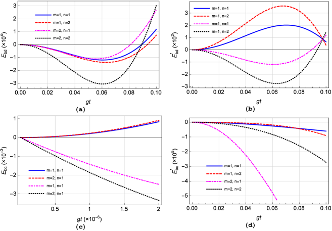
Figure 7: (Color online) The presence of lower and higher order entanglement in Stokes-anti-Stokes ((a)-(b)) and Stokes-vibration ((c)-(d)) modes is established using HZ1 ((a) and (c)) and HZ2 ((b) and (d)) criteria. The lower order entanglement in (a) is amplified 100 times, while higher order entanglement with $m=1,\,n=2$ is amplified 50 times. The dot-dashed-magenta and dotted-black lines in (b) and (c) correspond to the phase angle $\phi_{1}=\frac{\pi}{2}$ and $-\frac{\pi}{2}$, respectively, in $\alpha_{1}=\left|\alpha_{1}\right|\exp\left(i\phi_{1}\right)$. In (c), the lower order entanglement is shown after multiplying with 100, whereas in (d), the lower order entanglement is amplified 10 times and $m=1,\,n=2$ and $m=2,\,n=2$ are $10^{5}$ and $10^{3}$ times amplified, respectively. In all the cases, $\left|\alpha_{i}\right|=10$ has been used.

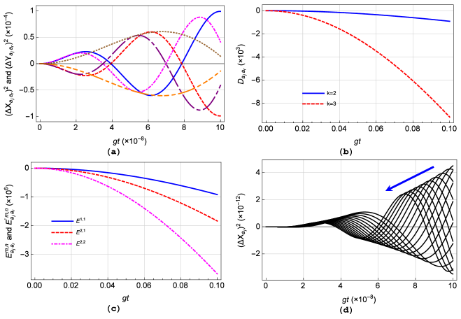
Figure 8: (Color online) The presence of lower and higher order nonclassicality in pump modes in spontaneous case. Intermodal (a) squeezing, (b) antibunching, and (c) entanglement for compound mode $a_{j}a_{r}$ is shown for the same values of the corresponding plots in Figures 2-6 for stimulated case. It is important to note that the values for HZ1 and HZ2 are obtained to be the same. In (d), squeezing in quadrature $X_{a_{j}}$ for 2-pump modes stimulated case with the value of frequency $\left(\frac{\omega_{i}}{g}\right)$ for $a_{j}$ mode varied between $35\times 10^{6}$ and $65\times 10^{6}$ in the steps of $2\times 10^{6}$. The arrow indicates the variation in quadrature squeezing due to increase in the frequency.

where

$$\begin{array}[]{lcl}F_{c+}&=&mn\sigma_{l}\left|\alpha_{j}\right|^{2\left(m-1\right)}\left|\gamma\right|^{2\left(n-1\right)}\left\{\left(n\left|\alpha_{j}\right|^{2}+m\left|\gamma\right|^{2}\right)\right.\\ &\times&\left.2\left|f_{3}\right|^{2}\left|\delta\right|^{2}+\left(mf_{2}^{*}f_{3}\beta^{*}\gamma^{*2}\delta+{\rm c.c.}\right)\right\}\end{array}$$

and $F_{c-}=0$; and

$$\begin{array}[]{lcl}\left(\begin{array}[]{c}E_{a_{j},d}^{m,n}\\ E_{a_{j},d}^{\prime m,n}\end{array}\right)&=&m\left|f_{3}\right|^{2}\left|\alpha_{j}\right|^{2\left(m-1\right)}\left(\left|\alpha_{i}\right|^{2}+\sigma_{l}\left(\left|\gamma\right|^{2}+1\right)\right)\\ &\times&\left|\delta\right|^{2n}\left(m\left|\delta\right|^{2}\mp n\left|\alpha_{j}\right|^{2}\right)+m^{2}\left|f_{2}\right|^{2}\left|\alpha_{j}\right|^{2\left(m-1\right)}\\ &\times&\left|\delta\right|^{2n}\left|\beta\right|^{2}\left|\gamma\right|^{2}\sigma_{l}+m\left|\alpha_{j}\right|^{2\left(m-1\right)}\left|\delta\right|^{2\left(n-1\right)}\sigma_{l}\\ &\times&\left\{\left(mf_{2}^{*}f_{3}\left|\delta\right|^{2}+nl_{4}^{*}l_{1}\left|\alpha_{j}\right|^{2}\right)\beta^{*}\gamma^{*2}\delta+{\rm c.c.}\right\},\end{array}$$ (20d)

respectively.

The analysis of the obtained analytic expressions of entanglement of an arbitrary pump mode with all the remaining modes revealed some interesting results. Specifically, all the pump modes are found to be entangled with vibration and anti-Stokes modes as shown in Figure 6 (b), (c) and (d). Importantly, the bipartite entanglement between a pump and vibration modes could only be ensured for initial evolution of the system. However, as the criteria used here are only sufficient not necessary, the separability of these two modes can not be deduced. One significant result, which would be absent in Raman or degenerate hyper-Raman process due to the existence of single pump mode, is entanglement between two pump modes (cf. Figure 6 (a)). The present results establish that two pump modes are always entangled in the non-degenarate hyper-Raman process. This interesting result would be in continuation of a set of systems able to produce always entangled pump modes Thapliyal et al. (2014a, b) and bosonic modes Giri et al. (2017).

A similar study for all the modes, except pump mode, resulted in following compact analytic expressions for Stokes-vibration, vibration-anti-Stokes, and Stokes-anti-Stokes modes

$$\begin{array}[]{lcl}\left(\begin{array}[]{c}E_{b,c}^{m,n}\\ E_{b,c}^{\prime m,n}\end{array}\right)&=&\left|g_{2}\right|^{2}\left|\beta\right|^{2\left(m-1\right)}\left|\gamma\right|^{2\left(n-1\right)}\left\{m^{2}\left(1\pm 2n\right)\left|\alpha_{i}\right|^{2}\left|\gamma\right|^{2}+n^{2}\left(1\pm 2m\right)\left|\alpha_{i}\right|^{2}\left|\beta\right|^{2}\right.\\ &\pm&\left.m^{2}n^{2}\left|\alpha_{i}\right|^{2}\mp mn\sigma_{l}\left|\beta\right|^{2}\left|\gamma\right|^{2}\right\}+n^{2}\left|h_{3}\right|^{2}\sigma_{l}\left|\beta\right|^{2m}\left|\gamma\right|^{2\left(n-1\right)}\left|\delta\right|^{2}\\ &\pm&mn\left|\beta\right|^{2\left(m-2\right)}\left|\gamma\right|^{2\left(n-2\right)}\left[g_{2}^{*}g_{1}\left|\beta\right|^{2}\left|\gamma\right|^{2}\alpha_{i}^{*}\beta\gamma+nh_{3}^{*}h_{2}\left|\beta\right|^{2}\left|\gamma\right|^{2}\alpha_{i}^{2}\beta^{*}\delta^{*}\right.\\ &+&g_{6}^{*}g_{1}\sigma_{l}\left|\beta\right|^{2}\beta\gamma^{2}\delta^{*}\left(2\left|\gamma\right|^{2}+n-1\right)+\left(n-1\right)h_{1}^{*2}h_{2}h_{3}\left|\alpha_{i}\right|^{2}\left|\beta\right|^{2}\beta^{*}\gamma^{*2}\delta\\ &+&\left.g_{2}^{*2}g_{1}^{2}\alpha_{i}^{*2}\beta^{2}\gamma^{2}\left\{\frac{1}{2}\left(m-1\right)\left(n-1\right)+\left(n-1\right)\left|\beta\right|^{2}+\left(m-1\right)\left|\gamma\right|^{2}\right\}+{\rm c.c.}\right],\end{array}$$ (20e)

$$\begin{array}[]{lcl}\left(\begin{array}[]{c}E_{c,d}^{m,n}\\ E_{c,d}^{\prime m,n}\end{array}\right)&=&m^{2}\left|h_{2}\right|^{2}\left|\alpha_{i}\right|^{2}\left|\gamma\right|^{2\left(m-1\right)}\left|\delta\right|^{2n}\\ &+&\left|l_{2}\right|^{2}\left|\gamma\right|^{2\left(m-1\right)}\left|\delta\right|^{2n}\sigma_{l}\left[m^{2}\left|\delta\right|^{2}\mp mn\left|\gamma\right|^{2}\right],\end{array}$$ (20f)

and

$$\begin{array}[]{lcl}\left(\begin{array}[]{c}E_{b,d}^{m,n}\\ E_{b,d}^{\prime m,n}\end{array}\right)&=&m^{2}\left|g_{2}\right|^{2}\left|\alpha_{i}\right|^{2}\left|\beta\right|^{2\left(m-1\right)}\left|\delta\right|^{2n}\\ &\pm&mn\left|\beta\right|^{2\left(m-1\right)}\left|\delta\right|^{2\left(n-1\right)}\left[l_{1}^{*}l_{3}\alpha_{i}^{2}\beta^{*}\delta^{*}+{\rm c.c.}\right],\end{array}$$ (20g)

respectively.

Entanglement between the modes except pump mode is also a topic of prime interest in some of the recent studies on Raman or degenerate hyper-Raman process Sen et al. (2013); Giri et al. (2016). The present results clearly reestablish that the non-separability criteria are only sufficient as one of the criteria (either HZ1 or HZ2) detects entanglement while the other one fails to detect entanglement in the same regimes of various parameters (cf. Figure 7 (a)-(b) or (c)-(d)). The present results show Stokes-anti-Stokes and Stokes-vibration modes are both lower and higher order entangled.

Finally, before we conclude the paper it is customary to check the possibility of nonclassical behavior that can be observed even under the spontaneous condition. The present results show that intermodal squeezing, antibunching and entanglement between different pump modes can be observed in the spontaneous case, too (cf. Figure 8). Here, in Figure 8 (d), we also establish the effect of change in frequency of input pump beams in spontaneous case, but it should be noted that a similar nature can be observed in stimulated case as well.

It is also worth noting here that in partial spontaneous case, when one (or two) of the modes except the pump modes has non-zero photons initially, all the nonclassicality observed in the spontaneous case will also survive. On top of that, certain other nonclassical behaviors may appear. Specifically, for non-zero photons in the Stokes mode, intermodal squeezing and antibunching in the pump-Stokes compound mode can also be observed.

V Conclusion

Here, we have obtained a completely quantum mechanical solution of the most general case of hyper-Raman process, i.e., with $k$ non-degenerate pump modes. Our endeavor to obtain the Sen-Mandal perturbative solution for this most general Hamiltonian, describing the multi-mode non-degenerate hyper-Raman process, resulted in a solution quite general in its nature. This general nature of the present Hamiltonian and corresponding solution insinuated to deduce all the existing Sen-Mandal and short time solutions for Raman and 2-pump mode degenerate hyper-Raman processes. This reduction establishes the wide applicability of the present results for all the Raman and hyper-Raman processes.

Further, the present study also revealed various interesting results. Specifically, the most significant property of the present system is more than one non-degenerate pump modes. Therefore, the nonclassical features reported in an arbitrary single pump and compound two-pump modes specify our most significant contribution. The present study revealed that an arbitrary single pump mode shows both lower and higher order squeezing and antibunching; while the compound pump-pump mode possesses all the nonclassical properties studied here, i.e., intermodal squeezing, antibunching, and entanglement.

The pump mode also shows compound mode nonclassicalities with Stokes, vibration, anti-Stokes modes as well. Specifically, compound pump-Stokes mode shows both intermodal squeezing and antibunching; compound pump-vibration mode exhibits intermodal squeezing and lower and higher order entanglement; intermodal squeezing antibunching, and lower and higher order entanglement are present in compound pump-anti-Stokes mode. Higher order entanglement in terms of multimode entanglement (as studied in Refs. Thapliyal et al. (2014a, b)) is not studied here as it is already shown that due to self-interaction two arbitrary pump modes are always entangled. Therefore, it is expected that all the pump modes would form a $k$-partite entangled state. In addition, all the nonclassical properties observed in Raman or degenerate hyper-Raman processes (Sen and Mandal (2005); Sen et al. (2007); Sen and Mandal (2007, 2008); Peřina (1991) and references therein) are also found to be present in the multi-mode non-degenerate hyper-Raman process. Precisely, the presence of intermodal antibunching and both lower and higher order entanglement in compound vibration-anti-Stokes and Stokes-anti-Stokes modes have been established.

Interestingly, most of the nonclassical properties of the hyper-Raman process under consideration survive even in the spontaneous case. To be specific, intermodal squeezing, antibunching, and lower and higher order entanglement between two arbitrary pump modes are observed in the spontaneous case. Further, squeezing and intermodal squeezing involving the pump mode are found to depend on the frequency and number of photons in the pump mode under consideration. It is also observed to vary with the number of non-degenerate pump modes. Additionally, intermodal antibunching and entanglement are phase dependent properties and can be controlled by the phases of the pump modes. The nonclassical behavior of hyper-Raman processes can also be established with the help of quasidistribution functions Thapliyal et al. (2015), which will be performed in the near future.

We conclude this paper with a hope that the growing experimental facilities and techniques would lead to experimental realization of the single mode and intermodal nonclassical properties observed in the pump and other modes in the present work.

Acknowledgment: KT acknowledges support from the Council of Scientific and Industrial Research, Government of India. AP thanks Department of Science and Technology (DST), India for the support provided through the project number EMR/2015/000393. JP thanks the support from LO1305 of the Ministry of Education, Youth and Sports of the Czech Republic.

Appendix A: Various terms in the obtained solution

The functional form of the coefficients in the evolution of various field modes given in Eq. (3) is as follows.

$$\begin{array}[]{lcl}f_{1}&=&\exp\left(-i\omega_{j}t\right),\\ f_{2}&=&-\frac{g^{*}f_{1}}{\Delta\omega_{1}}\left[\exp\left(-i\Delta\omega_{1}t\right)-1\right],\\ f_{3}&=&\frac{\chi f_{1}}{\Delta\omega_{2}}\left[\exp\left(i\Delta\omega_{2}t\right)-1\right],\\ f_{4}&=&-f_{5}=-f_{6}\\ &=&-\frac{|g|^{2}f_{1}}{\Delta\omega_{1}^{2}}\left[\exp\left(-i\Delta\omega_{1}t\right)-1\right]-\frac{i|g|^{2}tf_{1}}{\Delta\omega_{1}},\\ f_{7}&=&\frac{-\chi^{*}g^{*}f_{1}}{\Delta\omega_{2}}\left[\frac{\exp\left[-i\left(\Delta\omega_{1}+\Delta\omega_{2}\right)t\right]-1}{\Delta\omega_{1}+\Delta\omega_{2}}-\frac{\exp\left(-i\Delta\omega_{1}t\right)-1}{\Delta\omega_{1}}\right],\\ f_{8}&=&\frac{-\chi g^{*}f_{1}}{\Delta\omega_{2}}\left[\frac{\exp\left[-i\left(\Delta\omega_{1}-\Delta\omega_{2}\right)t\right]-1}{\Delta\omega_{1}-\Delta\omega_{2}}-\frac{\exp\left(-i\Delta\omega_{1}t\right)}{\Delta\omega_{1}}\right]\\ &-&\frac{\chi g^{*}f_{1}}{\Delta\omega_{1}}\left[\frac{\exp\left[-i\left(\Delta\omega_{1}-\Delta\omega_{2}\right)t\right]-1}{\Delta\omega_{1}-\Delta\omega_{2}}+\frac{\exp\left(i\Delta\omega_{2}t\right)}{\Delta\omega_{2}}\right],\\ f_{9}&=&\frac{-\chi gf_{1}}{\Delta\omega_{1}}\left[\frac{\exp\left[i\left(\Delta\omega_{1}+\Delta\omega_{2}\right)t\right]-1}{\Delta\omega_{1}+\Delta\omega_{2}}-\frac{\exp\left(i\Delta\omega_{2}t\right)-1}{\Delta\omega_{2}}\right],\\ f_{10}&=&f_{11}=-f_{12}\\ &=&\frac{-|\chi|^{2}f_{1}}{\Delta\omega_{2}^{2}}\left[\exp\left(i\Delta\omega_{2}t\right)-1\right]+\frac{i|\chi|^{2}tf_{1}}{\Delta\omega_{2}},\end{array}$$ (A.1)

$$\begin{array}[]{lcl}g_{1}&=&\exp\left(-i\omega_{b}t\right),\\ g_{2}&=&\frac{gg_{1}}{\Delta\omega_{1}}\left[\exp\left(i\Delta\omega_{1}t\right)-1\right],\\ g_{3}&=&\frac{\chi^{*}gg_{1}}{\Delta\omega_{2}}\left[\frac{\exp\left[i\left(\Delta\omega_{1}-\Delta\omega_{2}\right)t\right]-1}{\Delta\omega_{1}-\Delta\omega_{2}}-\frac{\exp\left(i\Delta\omega_{1}t\right)-1}{\Delta\omega_{1}}\right],\\ g_{4}&=&-g_{5}=\frac{-|g|^{2}g_{1}}{\Delta\omega_{1}^{2}}\left[\exp\left(i\Delta\omega_{1}t\right)-1\right]+\frac{i|g|^{2}tg_{1}}{\Delta\omega_{1}},\\ g_{6}&=&\frac{\chi gg_{1}}{\Delta\omega_{2}}\left[\frac{\exp\left[i\left(\Delta\omega_{1}+\Delta\omega_{2}\right)t\right]-1}{\Delta\omega_{1}+\Delta\omega_{2}}-\frac{\exp\left(i\Delta\omega_{1}t\right)-1}{\Delta\omega_{1}}\right],\end{array}$$ (A.2)

$$\begin{array}[]{lcl}h_{1}&=&\exp\left(-i\omega_{c}t\right),\\ h_{2}&=&\frac{gh_{1}}{\Delta\omega_{1}}\left[\exp\left(i\Delta\omega_{1}t\right)-1\right],\\ h_{3}&=&\frac{\chi h_{1}}{\Delta\omega_{2}}\left[\exp\left(i\Delta\omega_{2}t\right)-1\right],\\ h_{4}&=&-h_{5}=-\frac{|g|^{2}h_{1}}{\Delta\omega_{1}^{2}}\left[\exp\left(i\Delta\omega_{1}t\right)-1\right]+\frac{i|g|^{2}th_{1}}{\Delta\omega_{1}},\\ h_{6}&=&\frac{\chi gh_{1}}{\Delta\omega_{2}}\left[\frac{\exp\left[i\left(\Delta\omega_{1}+\Delta\omega_{2}\right)t\right]-1}{\Delta\omega_{1}+\Delta\omega_{2}}-\frac{\exp\left(i\Delta\omega_{1}t\right)}{\Delta\omega_{1}}\right]\\ &-&\frac{\chi gh_{1}}{\Delta\omega_{1}}\left[\frac{\exp\left[i\left(\Delta\omega_{1}+\Delta\omega_{2}\right)t\right]-1}{\Delta\omega_{1}+\Delta\omega_{2}}-\frac{\exp\left(i\Delta\omega_{2}t\right)}{\Delta\omega_{2}}\right],\\ h_{7}&=&-h_{8}=-\frac{|\chi|^{2}h_{1}}{\Delta\omega_{2}^{2}}\left[\exp\left(i\Delta\omega_{2}t\right)-1\right]+\frac{i|\chi|^{2}th_{1}}{\Delta\omega_{2}},\end{array}$$ (A.3)

$$\begin{array}[]{lcl}l_{1}&=&\exp\left(-i\omega_{d}t\right),\\ l_{2}&=&-\frac{\chi^{*}l_{1}}{\Delta\omega_{2}}\left[\exp\left(-i\Delta\omega_{2}t\right)-1\right],\\ l_{3}&=&\frac{\chi^{*}gl_{1}}{\Delta\omega_{1}}\left[\frac{\exp\left[i\left(\Delta\omega_{1}-\Delta\omega_{2}\right)t\right]-1}{\Delta\omega_{1}-\Delta\omega_{2}}+\frac{\exp\left(-i\Delta\omega_{2}t\right)-1}{\Delta\omega_{2}}\right],\\ l_{4}&=&\frac{\chi^{*}g^{*}l_{1}}{\Delta\omega_{1}}\left[\frac{\exp\left[-i\left(\Delta\omega_{1}+\Delta\omega_{2}\right)t\right]-1}{\Delta\omega_{1}+\Delta\omega_{2}}-\frac{\exp\left(-i\Delta\omega_{2}t\right)-1}{\Delta\omega_{2}}\right],\\ l_{5}&=&l_{6}=\frac{|\chi|^{2}l_{1}}{\Delta\omega_{2}^{2}}\left[\exp\left(-i\Delta\omega_{2}t\right)-1\right]+\frac{i|\chi|^{2}tl_{1}}{\Delta\omega_{2}},\end{array}$$ (A.4)

where $\Delta\omega_{1}=(\omega_{b}+\omega_{c}-\sum_{i=1}^{k}\omega_{i})$ and $\Delta\omega_{2}=(\sum_{i=1}^{k}\omega_{i}+\omega_{c}-\omega_{d})$ are detuning in Stokes and anti-Stokes generation processes. As differential equations of all the pump modes are similar, here, we have explicitly written the solution for $j$th pump mode only.

Appendix B: Sen Mandal Solution of the process

We know that the evolution of an operator in Heisenberg picture can be given by

$$a_{j}(t)=\exp(iHt)a_{j}(0)\exp(-iHt)$$ (B.1)

which on expansion gives

$$\begin{array}[]{lcl}a_{j}(t)&=&a_{j}(0)+it[H,a_{j}(0)]+(it)^{2}[H,[H,a_{j}(0)]]\\ &+&(it)^{3}[H,[H,[H,a_{j}(0)]]]+\ldots,\end{array}$$ (B.2)

where (in Sen-Mandal approach) we calculate different commutators until we obtain new terms as functions of annihilation or creation operators of different modes involved in the process. For instance, to obtain the evolution of an arbitrary pump mode ($a_{j}$) we obtain

$$\begin{array}[]{lcl}[H,a_{j}(0)]&=&\prod_{i=1:i\neq j}^{k}\left(-\omega_{j}a_{j}(0)+g^{*}a_{i}^{\dagger}(0)b(0)c(0)+\chi a_{i}^{\dagger}(0)c^{\dagger}(0)d(0)\right)\\ {}[H,[H,a_{j}(0)]]&=&\prod_{i=1:i\neq j}^{k}\left(\omega_{j}^{2}a_{j}(0)+g^{*}\left(-\omega_{j}+\omega_{i}-\omega_{b}-\omega_{c}\right)a_{i}^{\dagger}(0)b(0)c(0)\right.\\ &+&\chi\left(-\omega_{j}+\omega_{i}+\omega_{c}-\omega_{d}\right)a_{i}^{\dagger}(0)c^{\dagger}(0)d(0)-|g|^{2}\left(a_{j}(0)A_{l}b^{\dagger}(0)b(0)c^{\dagger}(0)c(0)\right.\\ &-&\left.a_{i}^{\dagger}(0)a_{i}(0)a_{j}(0)b(0)b^{\dagger}(0)-a_{i}^{\dagger}(0)a_{i}(0)a_{j}(0)c^{\dagger}(0)c(0)\right)\\ &-&|\chi|^{2}\left(a_{j}(0)a_{i}^{\dagger}(0)a_{i}(0)d^{\dagger}(0)d(0)+a_{j}(0)A_{l}c(0)c^{\dagger}(0)d^{\dagger}(0)d(0)-a_{i}^{\dagger}(0)a_{i}(0)a_{j}(0)c^{\dagger}(0)c(0)\right)\\ &-&\left.\chi^{*}g^{*}a_{j}(0)A_{l}b(0)c^{2}(0)d^{\dagger}(0)-\chi ga_{j}(0)A_{l}b^{\dagger}(0)c^{\dagger 2}(0)d(0)\right)\\ {}[H,[H,[H,a_{j}(0)]]]&=&\prod_{i=1:i\neq j}^{k}\sum_{i,m=1:i\neq j\neq m}^{k}\left(-\omega_{j}^{3}a_{j}(0)+g^{*}\left(\omega_{j}^{2}+\omega_{i}^{2}+\omega_{b}^{2}+\omega_{c}^{2}-\omega_{i}\omega_{j}\right.\right.\\ &+&\left.\omega_{j}\omega_{b}+\omega_{j}\omega_{c}+2\omega_{i}\omega_{m}-2\omega_{i}\omega_{b}-2\omega_{i}\omega_{c}+2\omega_{b}\omega_{c}\right)a_{i}^{\dagger}(0)b(0)c(0)\\ &+&\chi\left(\omega_{j}^{2}+\omega_{i}^{2}+\omega_{c}^{2}+\omega_{d}^{2}-\omega_{i}\omega_{j}-\omega_{j}\omega_{c}+\omega_{j}\omega_{d}+2\omega_{i}\omega_{c}\right.\\ &+&\left.2\omega_{i}\omega_{m}-2\omega_{i}\omega_{d}-2\omega_{c}\omega_{d}\right)a_{i}^{\dagger}(0)c^{\dagger}(0)d(0)\\ &-&|g|^{2}\left(2\omega_{j}+\omega_{i}-\omega_{b}-\omega_{c}\right)\left(a_{j}(0)A_{l}b^{\dagger}(0)b(0)c^{\dagger}(0)c(0)\right.\\ &-&\left.a_{i}^{\dagger}(0)a_{i}(0)a_{j}(0)b(0)b^{\dagger}(0)-a_{i}^{\dagger}(0)a_{i}(0)a_{j}(0)c^{\dagger}(0)c(0)\right)\\ &-&|\chi|^{2}\left(-2\omega_{j}+\omega_{i}+\omega_{c}-\omega_{d}\right)\left(a_{j}(0)a_{i}^{\dagger}(0)a_{i}(0)d^{\dagger}(0)d(0)\right.\\ &+&\left.a_{j}(0)A_{l}c(0)c^{\dagger}(0)d^{\dagger}(0)d(0)-a_{i}^{\dagger}(0)a_{i}(0)a_{j}(0)c^{\dagger}(0)c(0)\right)\\ &-&\chi^{*}g^{*}\left(-2\omega_{j}+\omega_{i}-2\omega_{b}-3\omega_{c}+\omega_{d}\right)a_{j}(0)A_{l}b(0)c^{2}(0)d^{\dagger}(0)\\ &-&\chi g\left(-2\omega_{j}+\omega_{i}+\omega_{b}+3\omega_{c}-2\omega_{d}\right)a_{j}(0)A_{l}b^{\dagger}(0)c^{\dagger 2}(0)d(0)\\ &+&\left.\chi g^{*}\left(-\omega_{b}-2\omega_{c}+\omega_{d}\right)a_{j}^{\dagger}(0)a_{i}^{\dagger 2}(0)b(0)d(0)\right).\end{array}$$ (B.3)

It is important to note here that not a single new function of creation and annihilation operators is obtained in all the commutators after the third term in Eq. (B.2), after neglecting the terms beyond quadratic powers of $g$, $\chi$ and their complex conjugates to remain consistent with the perturbative method.

All these different functions of creation and annihilation operators occurring in these commutators may now be used to write the obtained solution (3) with unknown time dependent coefficients (such as $f_{i}$). To obtain the functional form of these unknown coefficients we substitute the obtained solution given in Eq. (3) in Heisenberg’s equations of motion (2) for various field modes, one can easily obtain the coupled differential equations for all $f_{i}$, $g_{i},$ $h_{i},$ and $l_{i}$ as follows

$$\begin{array}[]{lcl}\dot{f}_{1}&=&-i\omega_{j}f_{1},\\ \dot{f}_{2}&=&-i\omega_{j}f_{2}+ig^{*}\prod_{i=2}^{k}\left(f_{1_{i}}^{*}\right)g_{1}h_{1},\\ \dot{f}_{3}&=&-i\omega_{j}f_{3}+i\chi\prod_{i=2}^{k}\left(f_{1_{i}}^{*}\right)h_{1}^{*}l_{1},\\ \dot{f}_{4}&=&-i\omega_{j}f_{4}+ig^{*}\prod_{i=2:i\neq l}^{k}\left(f_{1_{i}}^{*}f_{2_{l}}^{*}\right)g_{1}h_{1},\\ \dot{f}_{5}&=&-i\omega_{j}f_{5}+ig^{*}\prod_{i=2}^{k}\left(f_{1_{i}}^{*}\right)g_{1}h_{2},\\ \dot{f}_{6}&=&-i\omega_{j}f_{6}+ig^{*}\prod_{i=2}^{k}\left(f_{1_{i}}^{*}\right)g_{2}h_{1},\\ \dot{f}_{7}&=&-i\omega_{j}f_{7}+ig^{*}\prod_{i=2:i\neq l}^{k}\left(f_{1_{i}}^{*}f_{3_{l}}^{*}\right)g_{1}h_{1},\\ \dot{f}_{8}&=&-i\omega_{j}f_{8}+ig^{*}\prod_{i=2}^{k}\left(f_{1_{i}}^{*}\right)g_{1}h_{3}+i\chi\prod_{i=2}^{k}\left(f_{1_{i}}^{*}\right)h_{2}^{*}l_{1},\\ \dot{f}_{9}&=&-i\omega_{j}f_{9}+i\chi\prod_{i=2:i\neq l}^{k}\left(f_{1_{i}}^{*}f_{2_{l}}^{*}\right)h_{1}^{*}l_{1},\\ \dot{f}_{10}&=&-i\omega_{j}f_{10}+i\chi\prod_{i=2}^{k}\left(f_{1_{i}}^{*}\right)h_{3}^{*}l_{1},\\ \dot{f}_{11}&=&-i\omega_{j}f_{11}+i\chi\prod_{i=2:i\neq l}^{k}\left(f_{1_{i}}^{*}f_{3_{l}}^{*}\right)h_{1}^{*}l_{1},\\ \dot{f}_{12}&=&-i\omega_{j}f_{12}+i\chi\prod_{i=2}^{k}\left(f_{1_{i}}^{*}\right)h_{1}^{*}l_{2},\end{array}$$ (B.4)

$$\begin{array}[]{lcl}\dot{g}_{1}&=&-i\omega_{b}g_{1},\\ \dot{g}_{2}&=&-i\omega_{b}g_{2}+ig\prod_{i=1}^{k}\left(f_{1_{i}}\right)h_{1}^{*},\\ \dot{g}_{3}&=&-i\omega_{b}g_{3}+ig\prod_{i=1}^{k}\left(f_{1_{i}}\right)h_{3}^{*},\\ \dot{g}_{4}&=&-i\omega_{b}g_{4}+ig\prod_{i=1}^{k}\left(f_{1_{i}}\right)h_{2}^{*},\\ \dot{g}_{5}&=&-i\omega_{b}g_{5}+ig\prod_{i=1:i\neq l}^{k}\left(f_{1_{i}}f_{2_{l}}\right)h_{1}^{*},\\ \dot{g}_{6}&=&-i\omega_{b}g_{6}+ig\prod_{i=1:i\neq l}^{k}\left(f_{1_{i}}f_{3_{l}}\right)h_{1}^{*},\end{array}$$ (B.5)

$$\begin{array}[]{lcl}\dot{h}_{1}&=&-i\omega_{c}h_{1},\\ \dot{h}_{2}&=&-i\omega_{c}h_{2}+ig\prod_{i=1}^{k}\left(f_{1_{i}}\right)g_{1}^{*},\\ \dot{h}_{3}&=&-i\omega_{c}h_{3}+i\chi\prod_{i=1}^{k}\left(f_{1_{i}}^{*}\right)l_{1},\\ \dot{h}_{4}&=&-i\omega_{c}h_{4}+ig\prod_{i=1}^{k}\left(f_{1_{i}}\right)g_{2}^{*},\\ \dot{h}_{5}&=&-i\omega_{c}h_{5}+ig\prod_{i=1:i\neq l}^{k}\left(f_{1_{i}}f_{2_{l}}\right)g_{1}^{*},\\ \dot{h}_{6}&=&-i\omega_{c}h_{6}+ig\prod_{i=1:i\neq l}^{k}\left(f_{1_{i}}f_{3_{l}}\right)g_{1}^{*}\\ &+&i\chi\sum_{i=1:i\neq l}^{k}\left(f_{1_{i}}^{*}f_{2_{l}}^{*}\right)l_{1},\\ \dot{h}_{7}&=&-i\omega_{c}h_{7}+i\chi\prod_{i=1:i\neq l}^{k}\left(f_{1_{i}}^{*}f_{3_{l}}^{*}\right)l_{1},\\ \dot{h}_{8}&=&-i\omega_{c}h_{8}+i\chi\prod_{i=1}^{k}\left(f_{1_{i}}^{*}\right)l_{2},\end{array}$$ (B.6)

$$\begin{array}[]{lcl}\dot{l}_{1}&=&-i\omega_{d}l_{1}\\ \dot{l}_{2}&=&-i\omega_{d}l_{2}+i\chi^{*}\prod_{i=1}^{k}\left(f_{1_{i}}\right)h_{1}\\ \dot{l}_{3}&=&-i\omega_{d}l_{3}+i\chi^{*}\prod_{i=1}^{k}\left(f_{1_{i}}\right)h_{2}\\ \dot{l}_{4}&=&-i\omega_{d}l_{4}+i\chi^{*}\prod_{i=1:i\neq l}^{k}\left(f_{1_{i}}f_{2_{l}}\right)h_{1}\\ \dot{l}_{5}&=&-i\omega_{d}l_{5}+i\chi^{*}\prod_{i=1:i\neq l}^{k}\left(f_{1_{i}}f_{3_{l}}\right)h_{1}\\ \dot{l}_{6}&=&-i\omega_{d}l_{6}+i\chi^{*}\prod_{i=1}^{k}\left(f_{1_{i}}\right)h_{3}\end{array}$$ (B.7)

The solutions of these differential equations are obtained using the boundary conditions $F_{1}=1$ and $F_{i}=0\,\forall i\neq 1$ with $F=\left\{f,g,h,l\right\}$ and are listed in Appendix A. The obtained solution is expected to satisfy the equal time commutation relation (ETCR) as

$$\begin{array}[]{lcl}\left[a_{j}(t),a_{j}^{\dagger}(t)\right]&=&\prod_{i=1}^{k}\left[1+\left\{\left(f_{1}^{*}f_{4}+{\rm c.c.}\right)-|f_{2}|^{2}\right\}A_{l}\right.\\ &\times&b^{\dagger}(0)b(0)c^{\dagger}(0)c(0)+a_{i}^{\dagger}(0)a_{i}(0)\left(b(0)b^{\dagger}(0)\right.\\ &\times&\left\{\left(f_{1}^{*}f_{5}+{\rm c.c.}\right)+|f_{2}|^{2}\right\}+c^{\dagger}(0)c(0)\\ &\times&\left.\left\{\left(f_{1}^{*}f_{6}+f_{1}^{*}f_{12}+{\rm c.c.}\right)+|f_{2}|^{2}+|f_{3}|^{2}\right\}\right)\\ &+&\left\{\left(f_{7}^{*}f_{1}+f_{1}^{*}f_{9}-f_{2}^{*}f_{3}\right)A_{l}b^{\dagger}(0)c^{\dagger 2}(0)d(0)\right.\\ &+&\left.{\rm c.c.}\right\}+\left(\left\{\left(f_{1}^{*}f_{11}+{\rm c.c.}\right)-|f_{3}|^{2}\right\}A_{l}\right.\\ &\times&c(0)c^{\dagger}(0)+a_{i}^{\dagger}(0)a_{i}(0)\\ &\times&\left.\left.\left\{\left(f_{1}^{*}f_{10}+{\rm c.c.}\right)+|f_{3}|^{2}\right\}\right)d^{\dagger}(0)d(0)\right]\\ &=&1.\end{array}$$ (B.8)

Similarly, we can calculate ETCR for all other modes as follows

$$\begin{array}[]{lcl}\left[b(t),b^{\dagger}(t)\right]&=&\prod_{i=1}^{k}\left[1+\left\{\left(g_{1}^{*}g_{4}+{\rm c.c.}\right)-|g_{2}|^{2}\right\}a_{i}^{\dagger}(0)a_{i}(0)\right.\\ &+&\left.\left\{\left(g_{1}^{*}g_{5}+{\rm c.c.}\right)+|g_{2}|^{2}\right\}A_{l}c^{\dagger}(0)c(0)\right]\\ &=&1,\end{array}$$ (B.9)

$$\begin{array}[]{lcl}\left[c(t),c^{\dagger}(t)\right]&=&\prod_{i=1}^{k}\left[1+\left\{\left(h_{1}^{*}h_{4}+h_{1}^{*}h_{8}+{\rm c.c.}\right)\right.\right.\\ &-&\left.|h_{2}|^{2}+|h_{3}|^{2}\right\}a_{i}^{\dagger}(0)a_{i}(0)\\ &+&\left\{\left(h_{1}^{*}h_{5}+{\rm c.c.}\right)+|h_{2}|^{2}\right\}A_{l}b^{\dagger}(0)b(0)\\ &+&\left.\left\{\left(h_{1}^{*}h_{7}+{\rm c.c.}\right)-|h_{3}|^{2}\right\}A_{l}d^{\dagger}(0)d(0)\right]\\ &=&1,\end{array}$$ (B.10)

and

$$\begin{array}[]{lcl}\left[d(t),d^{\dagger}(t)\right]&=&\prod_{i=1}^{k}\left[1+\left\{\left(l_{1}^{*}l_{6}+{\rm c.c.}\right)+|l_{2}|^{2}\right\}a_{i}(0)a_{i}^{\dagger}(0)\right.\\ &+&\left.\left\{\left(l_{1}^{*}l_{5}+{\rm c.c.}\right)+|l_{2}|^{2}\right\}A_{l}c^{\dagger}(0)c(0)\right]\\ &=&1.\end{array}$$ (B.11)

We have also verified that various constants of motion for this system given in Ref. Peřina (1991) are satisfied by the present solution. Specifically, we have checked that $C_{1}=\left(a_{j}^{\dagger}(t)a_{j}(t)+b^{\dagger}(t)b(t)+d^{\dagger}(t)d(t)\right)$ is a constant of motion Peřina (1991) for an arbitrary pump mode, i.e.,

Multi-photon pump hyper-Raman case	Degenerate hyper-Raman case Sen and Mandal (2007)	Raman case Sen and Mandal (2005)
$g_{1}$	$g_{1}^{{}^{\prime}}$	$g_{1}^{{}^{\prime\prime}}$
$g_{2}$	$g_{2}^{{}^{\prime}}$	$g_{2}^{{}^{\prime\prime}}$
$g_{3}$	$g_{5}^{{}^{\prime}}$	$g_{3}^{{}^{\prime\prime}}$
$g_{4}$	$g_{8}^{{}^{\prime}}$	$g_{6}^{{}^{\prime\prime}}$
$g_{5}$	$g_{6}^{{}^{\prime}}$, $g_{7}^{{}^{\prime}}$	$g_{5}^{{}^{\prime\prime}}$
$g_{6}$	$g_{3}^{{}^{\prime}}$, $g_{4}^{{}^{\prime}}$	$g_{4}^{{}^{\prime\prime}}$
$h_{1}$	$h_{1}^{{}^{\prime}}$	$h_{1}^{{}^{\prime\prime}}$
$h_{2}$	$h_{2}^{{}^{\prime}}$	$h_{2}^{{}^{\prime\prime}}$
$h_{3}$	$h_{3}^{{}^{\prime}}$	$h_{3}^{{}^{\prime\prime}}$
$h_{4}$	$h_{8}^{{}^{\prime}}$	$h_{5}^{{}^{\prime\prime}}$
$h_{5}$	$h_{6}^{{}^{\prime}}$, $h_{7}^{{}^{\prime}}$	$h_{6}^{{}^{\prime\prime}}$
$h_{6}$	$h_{4}^{{}^{\prime}}$, $h_{5}^{{}^{\prime}}$	$h_{4}^{{}^{\prime\prime}}$
$h_{7}$	$h_{9}^{{}^{\prime}}$, $h_{10}^{{}^{\prime}}$	$h_{7}^{{}^{\prime\prime}}$
$h_{8}$	$h_{11}^{{}^{\prime}}$	$h_{8}^{{}^{\prime\prime}}$
$l_{1}$	$l_{1}^{{}^{\prime}}$	$l_{1}^{{}^{\prime\prime}}$
$l_{2}$	$l_{2}^{{}^{\prime}}$	$l_{2}^{{}^{\prime\prime}}$
$l_{3}$	$l_{3}^{{}^{\prime}}$	$l_{3}^{{}^{\prime\prime}}$
$l_{4}$	$l_{4}^{{}^{\prime}}$, $l_{5}^{{}^{\prime}}$	$l_{4}^{{}^{\prime\prime}}$
$l_{5}$	$l_{6}^{{}^{\prime}}$, $l_{7}^{{}^{\prime}}$	$l_{5}^{{}^{\prime\prime}}$
$l_{6}$	$l_{8}^{{}^{\prime}}$	$l_{6}^{{}^{\prime\prime}}$

Table B.I: The relationship among the various functions in the solution obtained here and the existing solutions for Raman and degenerate hyper-Raman processes for the functions in the evolution of modes except pump mode. Here, we have used a (two) prime(s) in the superscript of the functions $F_{i}$s to distinguish the present solution from the degenerate hyper-Raman (Raman) process.

$$\begin{array}[]{lcl}C_{1}&=&a_{j}^{\dagger}(t)a_{j}(t)+b^{\dagger}(t)b(t)+d^{\dagger}(t)d(t)\\ &=&\prod_{i=1}^{k}\left[a_{j}^{\dagger}(0)a_{j}(0)+b^{\dagger}(0)b(0)+d^{\dagger}(0)d(0)\right.\\ &+&\left\{\left(f_{1}^{*}f_{2}+g_{2}^{*}g_{1}\right)a_{i}^{\dagger}(0)b(0)c(0)+{\rm c.c.}\right\}\\ &+&\left\{\left(f_{1}^{*}f_{3}+l_{2}^{*}l_{1}\right)a_{i}^{\dagger}(0)c^{\dagger}(0)d(0)+{\rm c.c.}\right\}\\ &+&\left(f_{1}^{*}f_{4}+g_{1}^{*}g_{5}+{\rm c.c.}\right)A_{l}b^{\dagger}(0)b(0)c^{\dagger}(0)c(0)\\ &+&\left\{\left(f_{1}^{*}f_{6}+f_{1}^{*}f_{12}+{\rm c.c.}\right)+|g_{2}|^{2}+|l_{2}|^{2}\right\}\\ &\times&a_{i}^{\dagger}(0)a_{i}(0)c^{\dagger}(0)c(0)\\ &+&\left(f_{1}^{*}f_{5}+g_{1}^{*}g_{4}+{\rm c.c.}\right)a_{i}^{\dagger}(0)a_{i}(0)b^{\dagger}(0)b(0)\\ &+&\left\{\left(f_{1}^{*}f_{5}+{\rm c.c.}\right)+|g_{2}|^{2}\right\}a_{i}^{\dagger}(0)a_{i}(0)\\ &+&\left\{\left(f_{1}^{*}f_{7}+f_{9}^{*}f_{1}+g_{6}^{*}g_{1}+l_{4}^{*}l_{1}\right)\right.\\ &\times&\left.A_{l}b(0)c^{2}(0)d^{\dagger}(0)+{\rm c.c.}\right\}\\ &+&\left\{\left(f_{1}^{*}f_{8}+g_{3}^{*}g_{1}+l_{3}^{*}l_{1}\right)a_{i}^{\dagger 2}(0)b(0)d(0)+{\rm c.c.}\right\}\\ &+&\left(f_{1}^{*}f_{10}+l_{1}^{*}l_{6}+{\rm c.c.}\right)a_{i}^{\dagger}(0)a_{i}(0)d^{\dagger}(0)d(0)\\ &+&\left.\left(f_{1}^{*}f_{11}+l_{1}^{*}l_{5}+{\rm c.c.}\right)A_{l}c(0)c^{\dagger}(0)d^{\dagger}(0)d(0)\right]\\ &=&a_{j}^{\dagger}(0)a_{j}(0)+b^{\dagger}(0)b(0)+d^{\dagger}(0)d(0)\\ &=&{\rm constant}.\end{array}$$ (B.12)

Similarly, the present solution satisfies another constant of motion $C_{2}=a_{j}^{\dagger}(t)a_{j}(t)-a_{r}^{\dagger}(t)a_{r}(t)$ for two arbitrary pump modes, as follows

$$\begin{array}[]{lcl}C_{2}&=&a_{j}^{\dagger}(t)a_{j}(t)-a_{r}^{\dagger}(t)a_{r}(t)\\ &=&\prod_{i=1}^{r}\left[a_{j}^{\dagger}(0)a_{j}(0)-a_{r}^{\dagger}(0)a_{r}(0)\right.\\ &+&\left\{\left(f_{1}^{*}f_{2}-r_{1}^{*}r_{2}\right)a_{i}^{\dagger}(0)b(0)c(0)+{\rm c.c.}\right\}\\ &+&\left\{\left(f_{1}^{*}f_{3}-r_{1}^{*}r_{3}\right)a_{i}^{\dagger}(0)c^{\dagger}(0)d(0)+{\rm c.c.}\right\}\\ &+&\left(|f_{2}|^{2}-|r_{2}|^{2}\right)A_{l}b^{\dagger}(0)b(0)c^{\dagger}(0)c(0)\\ &+&\left(f_{1}^{*}f_{5}-r_{1}^{*}r_{5}+{\rm c.c.}\right)a_{i}^{\dagger}(0)a_{i}(0)b(0)b^{\dagger}(0)\\ &+&\left(f_{1}^{*}f_{6}+f_{1}^{*}f_{12}-r_{1}^{*}r_{6}-r_{1}^{*}r_{12}+{\rm c.c.}\right)\\ &\times&a_{i}^{\dagger}(0)a_{i}(0)c^{\dagger}(0)c(0)\\ &+&\left\{\left(f_{1}^{*}f_{7}+f_{9}^{*}f_{1}-r_{3}^{*}r_{2}\right)A_{l}b(0)c^{2}(0)d^{\dagger}(0)+{\rm c.c.}\right\}\\ &+&\left\{\left(f_{1}^{*}f_{8}-r_{1}^{*}r_{8}\right)a_{i}^{\dagger 2}(0)b(0)d(0)+{\rm c.c.}\right\}\\ &+&\left(f_{1}^{*}f_{10}-r_{1}^{*}r_{10}+{\rm c.c.}\right)a_{i}^{\dagger}(0)a_{i}(0)d^{\dagger}(0)d(0)\\ &+&\left.\left(|f_{3}|^{2}-|r_{3}|^{2}\right)A_{l}c(0)c^{\dagger}(0)d^{\dagger}(0)d(0)\right]\\ &=&a_{j}^{\dagger}(0)a_{j}(0)-a_{r}^{\dagger}(0)a_{r}(0)\\ &=&{\rm constant}.\end{array}$$ (B.13)

The last constant of motion $C_{3}=c^{\dagger}(t)c(t)+d^{\dagger}(t)d(t)-b^{\dagger}(t)b(t)$ is also verified as follows

$$\begin{array}[]{lcl}C_{3}&=&c^{\dagger}(t)c(t)+d^{\dagger}(t)d(t)-b^{\dagger}(t)b(t)\\ &=&\prod_{i=1}^{k}\left[c^{\dagger}(0)c(0)+d^{\dagger}(0)d(0)-b^{\dagger}(0)b(0)\right.\\ &+&\left\{\left(h_{1}^{*}h_{2}-g_{1}^{*}g_{2}\right)a_{i}(0)b^{\dagger}(0)c^{\dagger}(0)+{\rm c.c.}\right\}\\ &+&\left\{\left(h_{1}^{*}h_{3}+l_{2}^{*}l_{1}\right)a_{i}^{\dagger}(0)c^{\dagger}(0)d(0)+{\rm c.c.}\right\}\\ &+&\left\{\left(h_{1}^{*}h_{4}+h_{1}^{*}h_{8}+{\rm c.c.}\right)-|g_{2}|^{2}+|l_{2}|^{2}\right\}\\ &\times&a_{i}^{\dagger}(0)a_{i}(0)c^{\dagger}(0)c(0)\\ &+&\left(h_{1}^{*}h_{5}-g_{1}^{*}g_{5}+{\rm c.c.}\right)A_{l}b^{\dagger}(0)b(0)c^{\dagger}(0)c(0)\\ &+&\left(h_{1}^{*}h_{6}-g_{1}^{*}g_{6}+l_{4}^{*}l_{1}+{\rm c.c.}\right)A_{l}b^{\dagger}(0)c^{\dagger 2}(0)d(0)\\ &+&\left(l_{1}^{*}l_{9}-h_{1}^{*}h_{9}+k_{5}^{*}k_{1}+{\rm c.c.}\right)a_{2}^{\dagger}(0)a_{2}(0)\\ &\times&b^{\dagger}(0)c^{\dagger 2}(0)d(0)+\left(h_{1}^{*}h_{7}+l_{1}^{*}l_{5}+{\rm c.c.}\right)A_{l}\\ &\times&c^{\dagger}(0)c(0)d^{\dagger}(0)d(0)+\left(|h_{2}|^{2}-|g_{2}|^{2}\right)a_{i}^{\dagger}(0)a_{i}(0)\\ &+&\left\{\left(l_{1}^{*}l_{6}+{\rm c.c.}\right)+|h_{3}|^{2}\right\}a_{i}(0)a_{i}^{\dagger}(0)d^{\dagger}(0)d(0)\\ &+&\left.\left(h_{2}^{*}h_{3}-g_{3}^{*}g_{1}+l_{3}^{*}l_{1}+{\rm c.c.}\right)a_{i}^{\dagger 2}(0)b(0)d(0)\right]\\ &=&c^{\dagger}(0)c(0)+d^{\dagger}(0)d(0)-b^{\dagger}(0)b(0)\\ &=&{\rm constant}.\end{array}$$ (B.14)

It is previously mentioned that the present solution is general in nature and the solutions reported earlier for degenarate hyper-Raman process Sen and Mandal (2007) and Raman process Sen and Mandal (2005, 2008); Sen et al. (2011, 2007) can be obtained from the present solution as special cases. In Tables 1 and B.I, we have established a one-to-one correspondence between the functions obtained in the present solution and the same reported in the solutions for Raman and degenerate hyper-Raman processes.

References

• Abbott et al. (2016a) B. P. Abbott, R. Abbott, T. D. Abbott, M. R. Abernathy, F. Acernese, K. Ackley, C. Adams, T. Adams, P. Addesso, R. X. Adhikari, et al., Phys. Rev. Lett. 116, 061102 (2016a).
• Abbott et al. (2016b) B. P. Abbott, R. Abbott, T. D. Abbott, M. R. Abernathy, F. Acernese, K. Ackley, C. Adams, T. Adams, P. Addesso, R. X. Adhikari, et al., Phys. Rev. Lett. 116, 241103 (2016b).
• Ekert (1991) A. K. Ekert, Phys. Rev. Lett. 67, 661 (1991).
• Thapliyal and Pathak (2015) K. Thapliyal and A. Pathak, Quantum Inf. Process. 14, 2599 (2015).
• Thapliyal et al. (2017) K. Thapliyal, A. Pathak,  and S. Banerjee, Quantum Inf. Process. 16, 115 (2017).
• Bennett et al. (1993) C. H. Bennett, G. Brassard, C. Crépeau, R. Jozsa, A. Peres,  and W. K. Wootters, Phys. Rev. Lett. 70, 1895 (1993).
• Bennett and Wiesner (1992) C. H. Bennett and S. J. Wiesner, Phys. Rev. Lett. 69, 2881 (1992).
• Acin et al. (2006) A. Acin, N. Gisin,  and L. Masanes, Phys. Rev. Lett. 97, 120405 (2006).
• Hillery (2000) M. Hillery, Phys. Rev. A 61, 022309 (2000).
• Yuan et al. (2002) Z. Yuan, B. E. Kardynal, R. M. Stevenson, A. J. Shields, C. J. Lobo, K. Cooper, N. S. Beattie, D. A. Ritchie,  and M. Pepper, Science 295, 102 (2002).
• Pathak and Verma (2010) A. Pathak and A. Verma, Ind. J. Phys. 84, 1005 (2010).
• Sen and Mandal (2007) B. Sen and S. Mandal, J. Phys. B 40, 2901 (2007).
• Sen et al. (2011) B. Sen, V. Peřinová, A. Lukš, J. Peřina,  and J. Křepelka, J. Phys. B 44, 105503 (2011).
• Sen et al. (2007) B. Sen, S. Mandal,  and J. Peřina, J. Phys. B 40, 1417 (2007).
• Sen and Mandal (2005) B. Sen and S. Mandal, J. Mod. Opt. 52, 1789 (2005).
• Sen and Mandal (2008) B. Sen and S. Mandal, J. Mod. Opt. 55, 1697 (2008).
• Peřina (1991) J. Peřina, Quantum Statistics of Linear and Nonlinear Optical Phenomena (Kluwer Academic, Dordrecht-Boston, 1991).
• Miranowicz and Kielich (1994) A. Miranowicz and S. Kielich, “Quantum-statistical theory of Raman scattering processes,” in Modern Nonlinear Optics, Vol. 3 (John Wiley & Sons, New York, 1994) pp. 531–626.
• Peřinová et al. (1979a) V. Peřinová, J. Peřina, P. Szlachetka,  and S. Kielich, Acta Phys. Polonica A 56, 275 (1979a).
• Szlachetka et al. (1980) P. Szlachetka, S. Kielich, J. Peřina,  and V. Peřinová, J. Mod. Opt. 27, 1609 (1980).
• Peřinová and Tiebel (1984) V. Peřinová and R. Tiebel, Opt. Comm. 50, 401 (1984).
• Olivík and Peřina (1995) M. Olivík and J. Peřina, J. Mod. Opt. 42, 197 (1995).
• Peřinová et al. (1979b) V. Peřinová, J. Peřina, P. Szlachetka,  and S. Kielich, Acta Phys. Polonica A 56, 267 (1979b).
• Grangier (2005) P. Grangier, Nature 438, 749 (2005).
• Duan et al. (2001) L.-M. Duan, M. D. Lukin, J. I. Cirac,  and P. Zoller, Nature 414, 413 (2001).
• Rand (2013) S. C. Rand, J. Lumin. 133, 10 (2013).
• Freudiger et al. (2008) C. W. Freudiger, W. Min, B. G. Saar, S. Lu, G. R. Holtom, C. He, J. C. Tsai, J. X. Kang,  and X. S. Xie, Science 322, 1857 (2008).
• Sadler et al. (2007) L. E. Sadler, J. M. Higbie, S. R. Leslie, M. Vengalattore,  and D. M. Stamper-Kurn, Phys. Rev. Lett. 98, 110401 (2007).
• Bustard et al. (2011) P. J. Bustard, D. Moffatt, R. Lausten, G. Wu, I. A. Walmsley,  and B. J. Sussman, Opt. Exp. 19, 25173 (2011).
• Kielich (1993) S. Kielich, “Multi-photon scattering molecular spectroscopy,” in Progress in Optics, Vol. 20, edited by E. Wolf (Elsevier, Amsterdam, 1993) pp. 155–155.
• Ziegler (1990) L. D. Ziegler, J. Raman Spec. 21, 769 (1990).
• French and Long (1975) M. J. French and D. A. Long, J. Raman Spec. 3, 391 (1975).
• Valley et al. (2010) N. Valley, L. Jensen, J. Autschbach,  and G. C. Schatz, J. Chem. Phys. 133, 054103 (2010).
• Butet and Martin (2015) J. Butet and O. J. F. Martin, J. Phys. Chem. C 119, 15547 (2015).
• Kneipp et al. (2007) J. Kneipp, H. Kneipp, B. Wittig,  and K. Kneipp, Nano Lett. 7, 2819 (2007).
• Kockum et al. (2017) A. F. Kockum, A. Miranowicz, V. Macrì, S. Savasta,  and F. Nori, Phys. Rev. A 95, 063849 (2017).
• Kozich and Werncke (2007) V. Kozich and W. Werncke, J. Raman Spec. 38, 1180 (2007).
• Madzharova et al. (2017) F. Madzharova, Z. Heiner,  and J. Kneipp, Chem. Soc. Rev.  (2017).
• Thapliyal et al. (2014a) K. Thapliyal, A. Pathak, B. Sen,  and J. Peřina, Phys. Rev. A 90, 013808 (2014a).
• Thapliyal et al. (2014b) K. Thapliyal, A. Pathak, B. Sen,  and J. Peřina, Phys. Lett. A 378, 3431 (2014b).
• Thapliyal et al. (2016) K. Thapliyal, A. Pathak,  and J. Peřina, Phys. Rev. A 93, 022107 (2016).
• Szlachetka et al. (1979) P. Szlachetka, S. Kielich, J. Peřina,  and V. Peřinová, J. Phys. A 12, 1921 (1979).
• Miranowicz et al. (2010) A. Miranowicz, M. Bartkowiak, X. Wang, Y.-x. Liu,  and F. Nori, Phys. Rev. A 82, 013824 (2010).
• Peřina et al. (1984) J. Peřina, V. Peřinová,  and J. Koďousek, Opt. Comm. 49, 210 (1984).
• Sen et al. (2013) B. Sen, S. K. Giri, S. Mandal, C. H. R. Ooi,  and A. Pathak, Phys. Rev. A 87, 022325 (2013).
• Giri et al. (2016) S. K. Giri, B. Sen, A. Pathak,  and P. C. Jana, Phys. Rev. A 93, 012340 (2016).
• Richter and Vogel (2002) T. Richter and W. Vogel, Phys. Rev. Lett. 89, 283601 (2002).
• Allevi et al. (2012a) A. Allevi, S. Olivares,  and M. Bondani, Phys. Rev. A 85, 063835 (2012a).
• Allevi et al. (2012b) A. Allevi, S. Olivares,  and M. Bondani, Int. J. Quantum Inf. 10, 1241003 (2012b).
• Avenhaus et al. (2010) M. Avenhaus, K. Laiho, M. V. Chekhova,  and C. Silberhorn, Phys. Rev. Lett. 104, 063602 (2010).
• Hamar et al. (2014) M. Hamar, V. Michálek,  and A. Pathak, Meas. Sci. Rev. 14, 227 (2014).
• Peřina Jr. et al. (2017) J. Peřina Jr., V. Michálek,  and O. Haderka, Physical Review A 96, 033852 (2017).
• Loudon and Knight (1987) R. Loudon and P. L. Knight, J. Mod. Opt. 34, 709 (1987).
• Hong and Mandel (1985a) C. K. Hong and L. Mandel, Phys. Rev. Lett. 54, 323 (1985a).
• Hong and Mandel (1985b) C. K. Hong and L. Mandel, Phys. Rev. A 32, 974 (1985b).
• Hillery (1987) M. Hillery, Phys. Rev. A 36, 3796 (1987).
• Lee (1990) C. T. Lee, Phys. Rev. A 41, 1721 (1990).
• Pathak and Garcia (2006) A. Pathak and M. E. Garcia, Appl. Phys. B 84, 479 (2006).
• Hillery and Zubairy (2006a) M. Hillery and M. S. Zubairy, Phys. Rev. Lett. 96, 050503 (2006a).
• Hillery and Zubairy (2006b) M. Hillery and M. S. Zubairy, Phys. Rev. A 74, 032333 (2006b).
• Giri et al. (2017) S. K. Giri, K. Thapliyal, B. Sen,  and A. Pathak, Physica A 466, 140 (2017).
• Thapliyal et al. (2015) K. Thapliyal, S. Banerjee, A. Pathak, S. Omkar,  and V. Ravishankar, Ann. Phys. 362, 261 (2015).