Influence of thermal effects on stability of nanoscale films and filaments on thermally conductive substrates
Abstract
We consider films and filaments of nanoscale thickness on thermally conductive substrates exposed to external heating. Particular focus is on metal films exposed to laser irradiation. Due to short length scales involved, the absorption of heat in the metal is directly coupled to the film evolution, since the absorption length and the film thickness are comparable. Such a setup requires self-consistent consideration of fluid mechanical and thermal effects. We approach the problem via Volume-of-Fluid based simulations that include destabilizing liquid metal-solid substrate interaction potentials. These simulations couple fluid dynamics directly with the spatio-temporal evolution of the temperature field both in the fluid and in the substrate. We focus on the influence of the temperature variation of material parameters, in particular of surface tension and viscosity. Regarding variation of surface tension with temperature, the main finding is that while Marangoni effect may not play a significant role in the considered setting, the temporal variation of surface tension (modifying normal stress balance) is significant and could lead to complex evolution including oscillatory evolution of the liquid metal-air interface. Temperature variation of film viscosity is also found to be relevant. Therefore, the variations of surface tensions and viscosity could both influence the emerging wavelengths in experiments. In contrast, the filament geometry is found to be much less sensitive to a variation of material parameters with temperature.
I Introduction
Metal films of nanoscale thickness are of interest in numerous applications including solar cells, plasmonics related applications, sensing and detection among others. These applications include various geometries: particles, films, filaments and more complicated shapes. For a recent application-centered review, see Hughes et al. (2017); Makarov et al. (2016) for recent application-centered reviews. These films are typically exposed to a heat source (pulsed nanosecond laser) and, while in the liquid phase, evolve on a time scale measured in nanoseconds. This evolution is typically unstable due to the presence of destabilizing forces, in particular involving liquid metal-solid substrate interactions Bischof et al. (1996). In addition to its scientific interest, understanding these instabilities and the subsequent dynamics is further motivated by their potential to drive various self- and directed-assembly mechanisms in a variety of contexts; only some examples are cited here Ross (2010); Favazza et al. (2006); Xia and Chou (2009); Krishna et al. (2010); Fowlkes et al. (2014); Reinhardt et al. (2013).
A significant progress has been reached in understanding the instability mechanisms by considering essentially isothermal models that assume films and other geometries under isothermal conditions Kondic et al. (2009); Gonzalez et al. (2013a, b); Kondic et al. (2015); Mahady et al. (2016). In particular for the film geometry, the film-substrate interaction forces are crucial: a destabilizing force is needed for the instability to develop. In our earlier works, such a force has been included in the Navier-Stokes solver Mahady et al. (2015a, b), and the implemented approach is used in the present work as well. For filaments or other geometries that are characterized by limited spatial extent and the presence of contact lines, capillary effects are known to be dominant. In particular, for the commonly considered filament geometry, it has been shown that simply considering Rayleigh-Plateau instability mechanism with appropriately chosen material parameters (contact angle in particular) leads to satisfactory results, see, e.g. Diez et al. (2009a).
Clearly, the evolution of metal films and other geometries exposed to laser radiation is more complicated than that of an isothermal film. A laser pulse leads to a significant variation of the temperature field both in the film and in the substrate, resulting in phase change, and in variation of material parameters. The influence of such variation of material parameters with temperature on the stability of films and other metal geometries has been considered only to the limited extend so far Trice et al. (2007, 2008); Atena and Khenner (2009); Krishna et al. (2010); Dong and Kondic (2016). Furthermore, the existing studies, some of which we discuss next, have focused mostly on Marangoni effects, related to spatial variation of the film surface tension with temperature. We are not aware of any works in the present context that focus on the influence of temporal variation of surface tension (that is clearly relevant in the case of a time dependent laser pulse), or on the influence of variation of the film viscosity with temperature. These effects are among those discussed in the present work.
The Marangoni effect results from the spatial variation of tangential stresses due to temperature dependence of surface tension. In Trice et al. (2008), Marangoni effect is claimed to be responsible for the change of the average distances between the drops that form during pulse irradiation of metal films. For computing the temperature field, Ref. Trice et al. (2008) used the model, that we reference in the remaining part of this paper as ‘reduced’ model, that includes two important assumptions (i) that the temperature field is slaved to the film thickness, meaning essentially that the temperature is completely defined by the current value of the film thickness, and (ii) that the heat flux in the plane of the substrate can be ignored. Next, in a recent modeling and computational study Dong and Kondic (2016), the Marangoni effect was considered (within long wave limit) in a setup that relaxed the assumption (i) above, but still used the assumption (ii). In that work, it was found that the results were dramatically different compared to the ones obtained if the assumption (i) was used. In particular, a regime characterized by an oscillatory instability development has been found. This is in contrast to usual monotonic nature of instability evolution.
To summarize, the influence of thermal effects on the evolution of metal films and other geometries has not been studied extensively, and the results of the existing works are not always consistent. This motivates the present paper that focuses on providing further insight by carrying out careful and self-consistent simulations of the evolution of metal films and filaments. The considered approach is mainly computational and is based on a Volume-of-Fluid (VoF) method for solving the fluid mechanical problem, coupled with a thermal solver that computes the temperature field in the metal and in the substrate. Thin film (long wave) limit is used only for the purpose of obtaining basic insight via linear stability analysis, and the thermal problem is solved fully and self-consistently with the Navier-Stokes equations governing thin film evolution. In particular, the thermal problem considers both the in-plane and out-of-the-plane heat transport: we will see that for the setup considered, considering the in-plane heat diffusion is crucial. The VoF solver includes the interaction between metal and the substrate modeled via disjoining pressure approach Mahady et al. (2015b), as well as efficient calculation of tangential stresses and the resulting Marangoni effect that has been developed recently Seric et al. (2017). We note that in the present work, we discuss the phase change effects only indirectly, by limiting the metal film and filament evolution to the times for which metal temperature is above melting. Furthermore, we do not consider possible phase change of the substrate itself Font et al. (2017). Inclusion of these effects is left for future work.
The remainder of this paper is organized as follows. First, in Section II we formulate the governing equations coupling fluid mechanics with the thermal effects. We outline two temperature solutions used in the study of film breakup: first in Section II.1.1, we present a reduced model that ignores the in-plane heat conduction, as well as temporal evolution of the film or filament (referred to as the ‘reduced’ model’ from now on) Trice et al. (2007); and second in Section II.1.3, we present the numerical 2D temperature solution computed using Gerris (referred to as the ‘complete’ model’). In Section II.1.2, we outline an analytical solution for a flat film, which we use for validating and comparing the two models above. For definiteness, throughout the paper we use the parameters corresponding to nickel at the melting temperature, if not specified differently.
Section III presents the main findings. First, in Section III.1, using linear stability analysis (LSA) (in long wave limit), we find that the spatial temperature variations in the film can have a stabilizing or destabilizing effect depending on the film thickness: for films thinner than a critical value , the temperature variations have a stabilizing effect, and for the films of thickness larger than , the temperature variations have a destabilizing effect; such a critical value appears due to the nature of absorption of the laser energy by the film. Second, in Section III.2, using the direct numerical simulations, we consider the influence of temperature variation of surface tension on stability of a film, for the reduced and complete temperature models. We find that for the reduced model the relevance of Marangoni effect is exaggerated due to the lack of in-plane heat conduction. Furthermore, we find that, compared to the spatial variations leading to Marangoni effect, the temporal variation of surface tension has significantly stronger effect on the film stability; in other words, the balance of normal stresses (and its dependence on temperature) play much more important role than the variation of tangential stresses that lead to Marangoni effect. The temporal variation of the temperature is found also to influence the film evolution via temperature dependence of viscosity; this effect is discussed in Section III.3. Section III.4 is devoted to a brief discussion of the expected influence of temperature variation of material properties in physical experiments. Finally, in Section III.5, we consider the influence of the thermal effects on the breakup of the liquid metal filaments. We find that the influence of thermal effects is weak compared to the capillary ones governing the Rayleigh-Plateau type of instability. The paper is concluded by Section III.6, where we also discuss some directions for the future work.
II Governing Equations and Numerical Methods
We represent the two-phase flow by the Navier-Stokes equations, where the material properties are phase dependent; additional energy equation is discussed later in this section. The surface forces at the interface between two fluids are represented by a body force using the Continuum Surface Force (CSF) method Brackbill et al. (1992a); Francois et al. (2006); Afkhami and Bussmann (2009); Popinet (2009). Hence, the equations governing the flow are
| (1) | |||
| (2) |
and the advection of the phase-dependent density
| (3) |
where is the fluid velocity, is the pressure, and are the phase dependent density and viscosity respectively. is the rate of deformation tensor, . Subscripts and correspond to the fluids and , respectively (see Fig. 1). Here, is the characteristic function, such that in the fluid , and in the fluid . Note that any body force can be included in F. The characteristic function is advected with the flow, thus
| (4) |
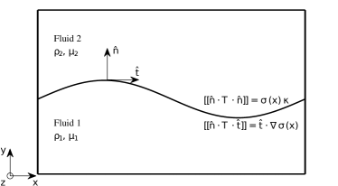
The presence of an interface gives rise to the stress boundary conditions, see Fig. 1. The normal stress boundary condition at the interface defines the stress jump (Landau and Lifshitz, 1987; Levich and Krylov, 1969)
| (5) |
where is the total stress tensor, is the surface tension, is the curvature of the interface, and is the unit normal at the interface pointing out of the fluid . The variation of surface tension results in the tangential stress jump at the interface
| (6) |
which drives the flow from the regions of low surface tension to the ones with high surface tension. Here, is the unit tangent vector in two dimensions (2D); in three dimensions (3D) there are two linearly independent unit tangent vectors. Using the CSF method (Brackbill et al., 1992b), the forces resulting from the normal and tangential stress jump at the interface can be included in the body force , defined as
| (7) |
and
| (8) |
where is the Dirac delta function centered at the interface, , and is the surface gradient. The details of the computations of the interfacial curvature and normals in the VoF method can be found in (Popinet, 2009), and the implementation of the surface gradients of the surface tension in (Seric et al., 2017).
The destabilizing mechanism leading to breakup of nanoscale films is modeled by the fluid-solid interaction in the form of a disjoining pressure Mahady et al. (2016). The disjoining pressure can be included in the Navier-Stokes equations (1) as a body force specified by
| (9) | |||
| (10) | |||
| (11) |
where is the surface tension of nickel at the melting temperature, and is the prescribed equilibrium contact angle. We use the exponents and as in Mahady et al. (2016); see also Gonzalez et al. (2013a); Ajaev and Willis (2003) and the references therein for further discussion regarding disjoining pressure models for metal films. The equilibrium film thickness used is nm, comparable to the values discussed in Mahady et al. (2016). Hence, the complete Navier-Stokes equations with the surface forces are as follows
| (12) |
The details of the implementation of the disjoining pressure in the VoF method can be found in (Mahady et al., 2015a).
II.1 Temperature Models
The variations of the temperature of a liquid metal film exposed to a pulsed laser can be caused by spatial variability of the pulse itself. However, since the spatial scale of the pulse is typically few orders of magnitude larger than any other relevant length scale Gonzalez et al. (2013a), we consider a spatially homogenous pulse where a temperature variation may result from variable film thickness. This is due to fact that the optical (and energy absorption) properties of the metal depend on the film thickness Heavens (1991), as we will discuss in what follows.
We start this section by considering a simplified (‘reduced’) model that ignores various aspects of the heat flow, such as heat transport in the in-plane direction, as well as the convective effects. In Section II.1.1 a numerical solution of such a model, that has been previously used in the context of metal films Trice et al. (2007, 2008) is discussed, and in Section II.1.2, an analytical solution of the underlying one-dimensional model for heat transport is presented. Complete numerical solution of the energy equation is given in Section II.1.3. The comparison of the results obtained using these approaches will allow to gain better insight into the most important factors determining temperature distribution.
II.1.1 Reduced Model for the Temperature of a Thin Film
In this section, we outline the reduced model for the metal temperature; a version of such model is discussed in (Trice et al., 2007). The film–substrate bilayer is assumed to be infinitely wide in the in-plane directions. The substrate layer is assumed to be thick compared to the film thickness and it is modeled as a semi-infinite medium . Assuming that any variation of film thickness occurs on the scale which is much larger than the film thickness, one could argue that the heat conduction in the in–plane direction in the film is negligible compared to the conduction in the out-of-plane direction. Although the same argument does not apply to a (thick) substrate, it is still assumed to hold. Hence, within this reduced model, the heat conduction in the bilayer is described by the one-dimensional heat equation in each layer,
| (13) | ||||
| (14) |
where is the effective heat capacity and is the thermal conductivity. The subscripts and correspond to substrate and metal, respectively. The source term can be written as
| (15) |
where the first factor represents the incident energy from the laser source, second factor accounts for the reflectance of the metal film, and the last factor represents the energy absorbed by the film. In Eq. (15), is the intensity of the incident radiation, is the width of the Gaussian laser pulse at half maximum, and gives the temporal profile of the laser fluence,
| (16) |
More details regarding the derivation of the source term and the explanation of the parameters are given in Appendix A; the parameters themselves are specified in Tab. 1. The boundary conditions are as follows
| (17) | ||||
| (18) | ||||
| (19) | ||||
| (20) |
where corresponds to the film-air interface, and is the film-substrate interface.
| Description | Notation | Value/Expression |
|---|---|---|
| Density of the metal | kg/m3 | |
| Density of the substrate | kg/m3 | |
| Room temperature | K | |
| Melting temperature of the metal | K | |
| Viscosity of the metal at | Pa s | |
| Surface tension | ||
| Reference surface tension | N/m | |
| Change of with respect to temperature | N/m K | |
| Conductivity of the metal | W/m K | |
| Conductivity of the substrate | W/m K | |
| Heat capacity of the metal | J/kg K | |
| Heat capacity of the substrate | J/kg K | |
| Laser fluence | J/m2 | |
| Time of maximum fluence | s | |
| Absorption length | m-1 | |
| Fit parameter for reflectance | ||
| Fit parameter for reflectance | m)-1 | |
| Equilibrium contact angle of metal with substrate | ||
| Exponents in in the disjoining pressure model | ||
| Precursor film thickness | m |
The spatial variation of the temperature in the metal film is expected to be small due to the small film thickness and high thermal conductivity of the metal. Hence, within this model, it can be assumed that the temperature only weakly depends on the -coordinate, and the temperature of the film-air interface can be approximated by the average film temperature, . Integrating Eq. (13) with respect to , from to , and using the boundary conditions (17) and (18), gives the equation for the average temperature of the film,
| (21) | ||||
| (22) |
where
The heat equation for the substrate (14) can be solved using Green’s functions or Laplace transform. Using the boundary conditions (18), (19) and (20), the average temperature of the film is found to be
| (23) |
where is the complementary error function and
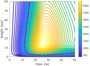
Figure 2 shows the contour plot of the average temperature of the metal film, , as given by Eq. (23). The red highlighted curve represents the melting temperature of nickel . We note that the energy absorption depends on the film thickness in a non-monotonic manner. For a small film thickness, nm, only a part of the laser energy is absorbed, which leads to low film temperature. For film thicknesses the film absorbs most of the laser pulse energy. Hence, the film of thickness reaches the highest temperature, and for the film of thicknesses , the temperature decreases as grows due to the larger amount of material that needs to be heated. Later in Sections III.1 and III.2, we study the dynamics of the films with the film thickness either smaller or larger than .
A known temperature at the interface which is expressed as a function of the film thickness, , and time, only, is convenient for implementing the Marangoni force in the VoF solver. The surface gradients of the surface tension, , can be evaluated directly as
| (24) |
where is the arc length, and is the height function Francois and Swartz (2010); Seric et al. (2017). As discussed earlier, is approximated by the average temperature , and therefore the gradient of the temperature with respect to the film thickness is approximated by that can be computed analytically from Eq. (23) as follows
| (25) |
Note that in Eq. (24), is equivalent to , i.e., the derivative of the height function. For small film thicknesses, and need to be carefully computed to ensure that the integrals in Eqs. (23) and (25) converge, see Appendix B. When used in our simulations, both and are evaluated for an array of and values before the start of the simulations. During the simulation, we use bilinear interpolation to find the temperature at each interfacial cell and each time step. This makes the computations significantly faster, since we do not need to use the numerical integration to compute the integrals in Eqs. (23) and (25) for each interfacial cell at each time step.
II.1.2 Analytical Solution of the Heat Equation in a Film–Substrate System
The Eqs. (13) and (14), including the spatial variations in the -direction in both the metal and the substrate, can be solved analytically using separation of variables, following the technique given in (Özışık, 1989). The analytical solution presented here is used for the verification of the reduced model given in Eq. (23) and the complete model is presented in Section II.1.3.
In contrast to the reduced model presented in Section II.1.1, for computing the analytical solution, we assume that the substrate is of finite depth. However, when comparing the solutions resulting from different models, we use substrate depth large enough so that the temperature solution is converged with increasing substrate thickness, and the solution is equivalent to that for the semi-infinite substrate (see Fig. 24 in Appendix C). Therefore, instead of Eq. (20), here we use the following boundary condition
| (26) |
where is the substrate thickness.
The solution can be found using separation of variables (Özışık, 1989), and it can be written compactly in terms of Green’s functions as
| (27) | ||||
| (28) |
where and are given in Appendix C along with the details of the solution.
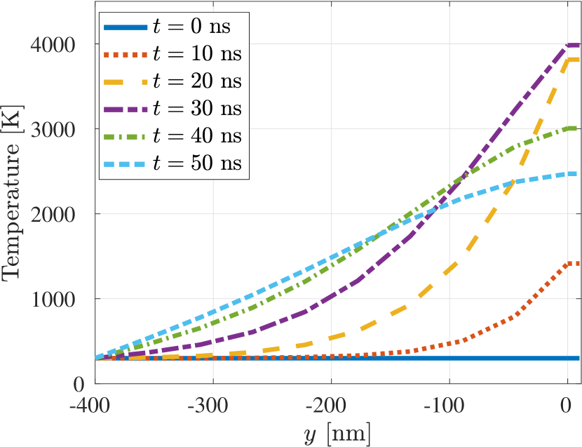
Figure 3 shows the analytical temperature solution in the metal film () and the substrate (). The temperature variation across the film thickness is small compared to the variation in the substrate. Therefore, ignoring temperature gradients across the film, as used in the reduced model, is justified. We note, however, that such a conclusion can be reached only for stationary flat films. As we will see later, using the reduced model for nonuniform films, or for the time dependent films, in general cannot be justified. On a different note, we point out that since there is no in-plane dependence in the source term, the 1D analytical solution presented here holds for 2D or 3D flat stationary films.
II.1.3 Computational Model for the Temperature of the Film–Substrate System
Next we consider the outlined problem via direct numerical simulations. We implement our numerical methods into the open source Gerris software Popinet (2013-12-06). We denote the top subdomain containing metal and air by , and the bottom one containing the substrate by . In general, the temperature in , denoted , satisfies the advection-diffusion equation, and the temperature in , , satisfies the diffusion equation,
| (29) | ||||
| (30) |
where , and are the phase dependent density, heat capacity and the conductivity of the metal and air, defined as the volume fraction weighted average of the metal and air properties.
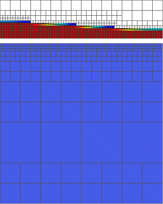
The simulation setup has to address the following issue: using Gerris we cannot solve for the temperature inside of the solid substrate directly, since except on the boundaries, the implementation of the solid entities does not contain the computational cells. Hence, in order to solve for the temperature in the fluid and the substrate using Gerris, we treat the solid domain – the substrate – as an immobile fluid. Furthermore, in order to impose the no-slip boundary condition on the metal-substrate boundary, we separate the two phases by a thin solid plate, see Fig. 4. Later in this section we show by direct comparison with the analytical solution that this setup, referred to as the complete model, produces correct results.
The coupling of the temperature solution between the liquid and solid domains is accomplished using Newton’s law of cooling, which we impose on the top and bottom of the solid plate as follows
| (31) | ||||
| (32) |
where is the heat transfer coefficient. Note that the right hand sides of Eqs. (31) and (32) are equal, implying the continuity of the flux between the liquid and substrate. Furthermore, in the limit , the boundary conditions (31) and (32) both imply . Hence, the boundary conditions specified by Eqs. (31) and (32) effectively encapsulate both the continuity of flux, Eq. (18), and the continuity of temperature, Eq. (19). Additionally, in Appendix C, see Fig. 25, we confirm that the analytical solution, given in Section II.1.2, with the Newton’s cooling law boundary condition, converges for large to the solution specified by requiring continuity of temperature. We note that the presented computational approach can be used for arbitrary metal-air interface shape.
In the remainder of this section, we verify that the numerical solutions to Eqs. (29) and (30), along with the boundary conditions, Eqs. (31) and (32), converge with the increasing heat transfer coefficient, , and the substrate thickness, . To do this, we consider the following test problem. Assume the metal-air interface is flat and the solution is -independent. Hence, the temperature for the 2D problem satisfies the 1D heat equation at any fixed position , and the 1D analytical solution, presented in Section II.1.2, holds. We compare the temperature solution obtained from the complete model to the 1D analytical solution, where we average the temperature over the film thickness for the purpose of this comparison.
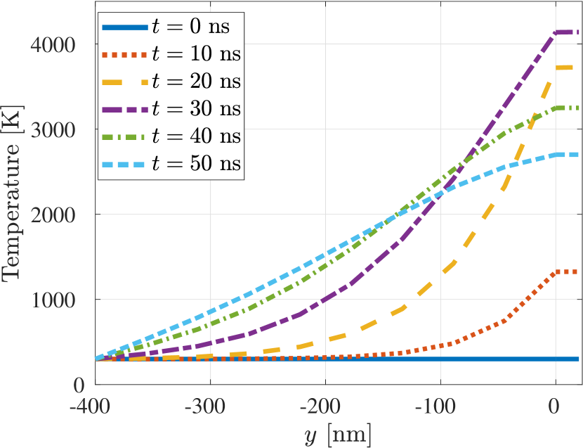
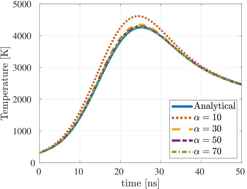
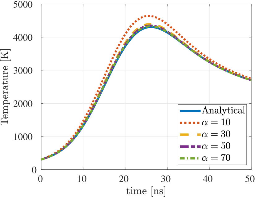
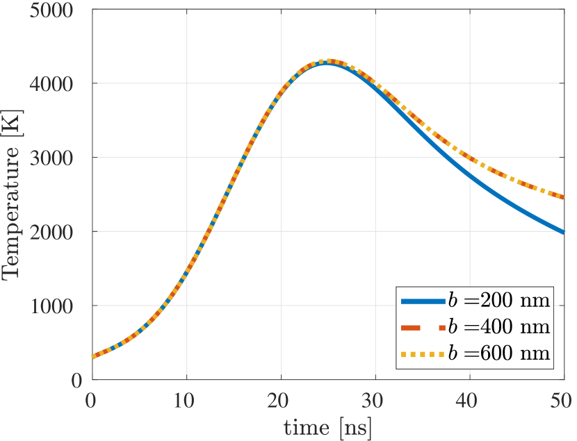
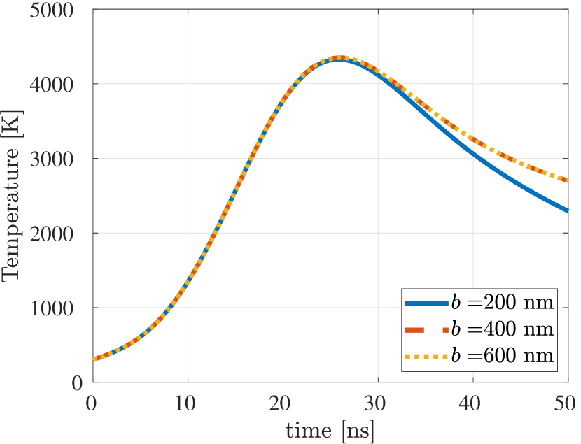
Figure 5 shows the temperature solution of the complete model for a flat film geometry and vanishing velocity in Eq. (29) compared to the analytical solution for increasing values of . Clearly, as increases, the results of the complete model approach the analytical solution. The largest relative difference in the temperature between and is for a nm, and for a nm. Since larger decreases the required time-step, we use in order to reduce the computational time. Figure 6 shows the convergence of the solution of the complete model for the averaged temperature for increasing substrate size, . The largest relative difference in the temperature between nm and nm is for a nm, and for a nm. We conclude that it is sufficient to use nm.
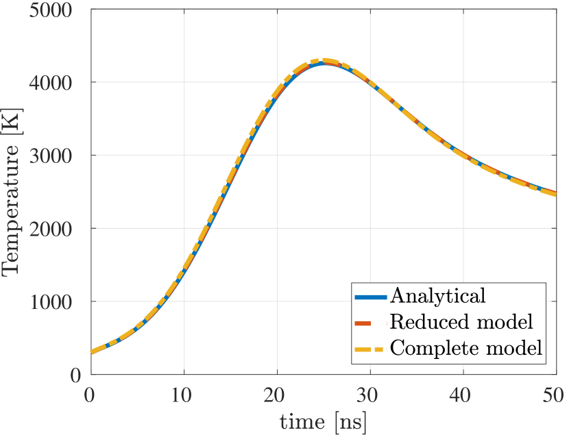
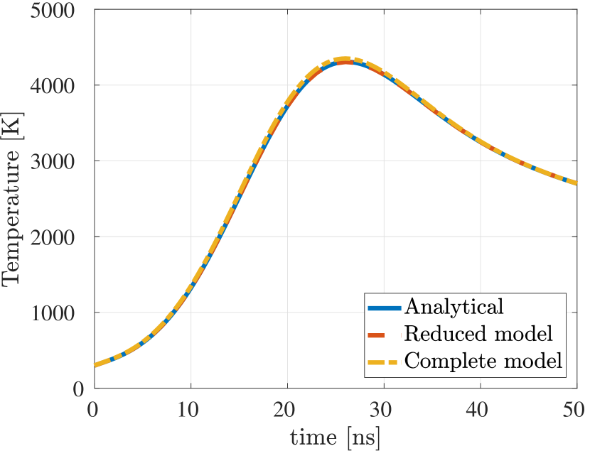
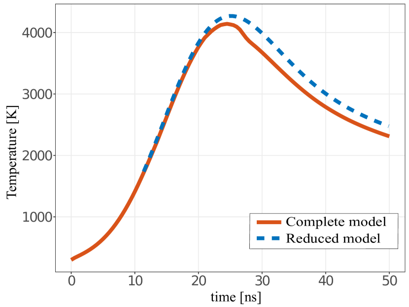
So far, we have shown that the solution to the complete model described in this section converges with the increased heat transfer coefficient, , and the substrate thickness, , to the analytical solution with continuity of temperature boundary condition at the fluid-substrate interface. Next, Fig. 7 shows the comparison of the average temperature in the metal film obtained using the reduced model given in Section II.1.1, the analytical solution outlined in Section II.1.2, and the complete model described in this section. The average temperature of a flat metal film in both the reduced and the complete model agrees with the analytical solution. Hence, we are confident in the numerical implementation of the temperature models in our numerical solver.
We point out this agreement between different models, in particular the reduced and complete model holds only for flat films for which the heat flow in the in-plane direction is not relevant. For perturbed films, the two models produce different results, as we will discuss in the next section.
III Results and Discussion
We are now ready to discuss the influence of thermal effects on the film stability. First in Sections III.1 - III.4 we focus on film geometry, and then consider filaments in Section III.5. We start by discussing briefly in Section III.1 the results of linear stability analysis carried out within the long wave limit in a simplified setting (that assumes film temperature to be dependent only on the current value of the film thickness). Then, we follow in Section III.2 by presenting the results using the models for temperature computation outlined in the preceding section. We will see that the outcomes of the models considered differ significantly. The main finding is that the reduced model overestimates the Marangoni effect, and the particular reason for this is the omission of the in-plane heat conduction. We will also see that the temporal temperature variations lead to a change in the surface tension, which can in turn affect the stability of the perturbed interface during the evolution. As we will see, the interplay of the stabilizing/destabilizing Marangoni effect and temporal variation of surface tension leads to a complex form of film evolution. In Section III.3 we consider also temperature variation of film viscosity, and its influence on the film stability. Section III.5 discusses the influence of thermal effects on stability of metal filaments.
For both films and for filaments, we focus on developing basic understanding of the influence of thermal effects on their stability. Therefore, we focus on relatively simple computational domains and initial conditions - in particular, in simulations we will consider films and filaments perturbed by a single wavelength, and defer considering more complex domains and initial conditions to future work. As we will see, even for simple setups the influence of variation of material parameters (surface tension and viscosity) is rather complex, and the simplicity of the considered computational domains and initial conditions helps in focusing on the basic questions. In addition, we focus on the question of stability versus instability of a given perturbation; for this reason in our simulations we choose initial conditions that are close to the critical ones where stability changes: such a choice helps to further simplify the problem considered and reach answers to the basic stability questions.
III.1 Linear Stability Analysis of a Thin Film in Two Dimensions
First, to gain basic insight, we present the results of linear stability analysis (LSA) carried out within the long wave limit. While the LSA provides only approximate results since (i) it is valid only for early stages of instability, and (ii) corresponds to the long wave limit, we still expect it to provide a useful insight.
The long wave limit Oron et al. (1997), for a Newtonian film with Marangoni effect and the fluid-substrate interaction in the form of the disjoining pressure Diez and Kondic (2007) leads to the following 4th order nonlinear partial differential equation
| (33) | |||
where is given by Eq. (10). We assume the film thickness is perturbed around the equilibrium one, , as
| (34) |
where is a small parameter, is the growth rate of the perturbation and is the wavenumber. Note that temperature is not an independent variable here, instead it is a function of . An alternative approach is to consider both and as independent variables, and perturb each of them separately, however, we are not doing this here for simplicity. Keeping only the leading order terms in we obtain the dispersion relation:
| (35) |
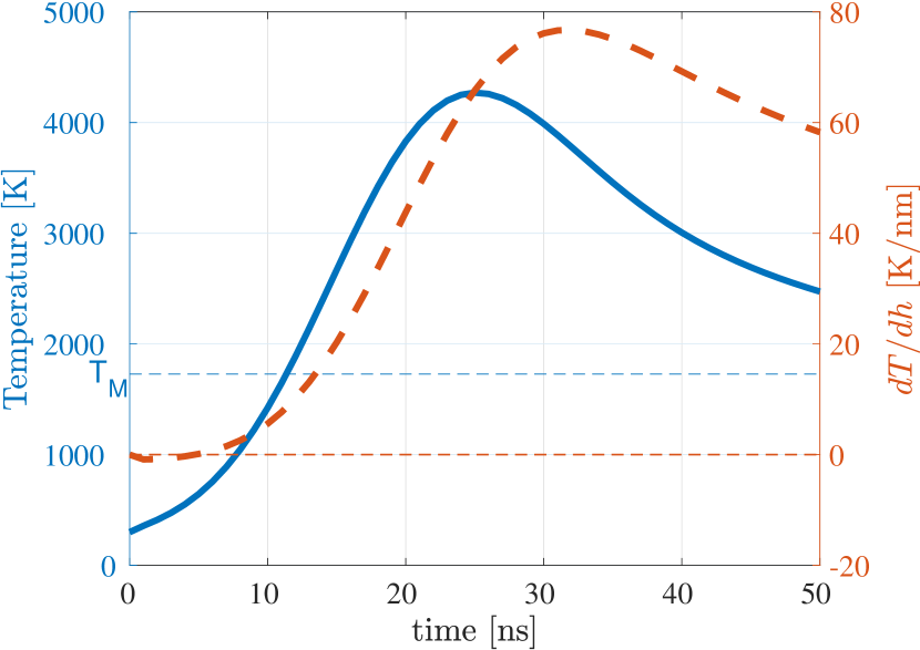
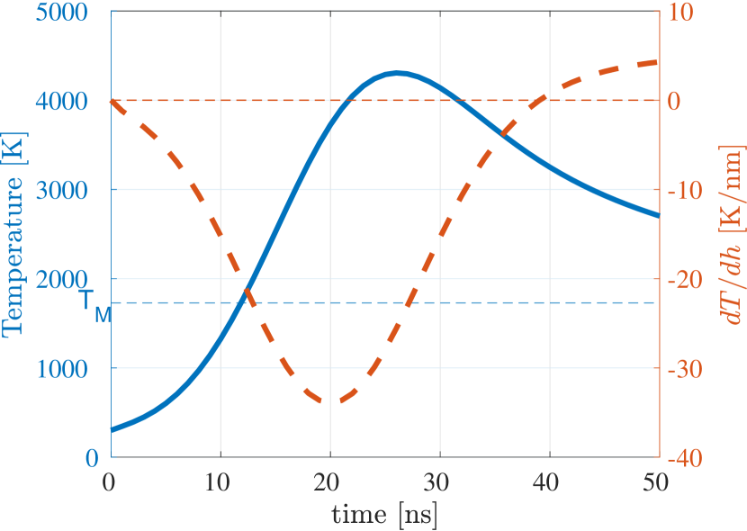
To illustrate the expected influence of Marangoni effect on stability, in Fig. 8 we plot the temperature gradient, , for a fixed film thickness computed using the reduced model (see Eq. (25)). The temperature of the film, (see Eq. (23)), is plotted to show the film melting time. We assume that before the temperature of the film rises above , the film does not evolve. The value of the gradient changes as a function of time, and in order to obtain an estimate for the stability of a perturbed film using Eq. (35), we approximate by the largest absolute value of , during the time the film is melted. Hence, the obtained dispersion curve provides the upper bound on the influence of the Marangoni effect.
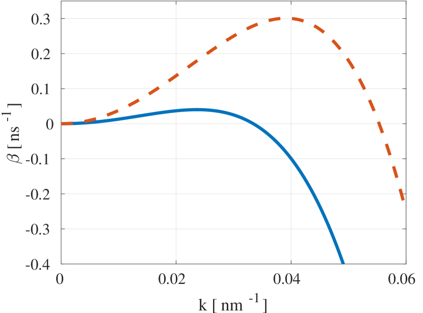
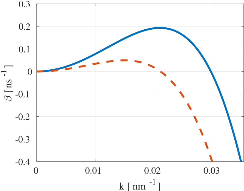
Figure 9 shows the dispersion curve for and nm thick films. For the nm thick film, Fig. 9(a), the Marangoni effect is stabilizing, since , for all the times at which the film is melted. Conversely, for nm film, Fig. 9(b), the Marangoni effect is destabilizing for a significant period after melting, since .
In the rest of this section, we will use the outlined LSA results to rationalize the results computed using the reduced and complete models for the flow of thermal energy.
III.2 Evolution of a Thin Film Interface in Two Dimensions
In this section, we examine the stability of the films by solving the Navier-Stokes equations including the thermal effects. We also include the fluid-substrate interaction in the form of a disjoining pressure (see Eq. (12)). We compare the influence of thermal effects on the film breakup using the temperature solution from the reduced and from the complete model, described in Sections II.1.1 and II.1.3, respectively.
The initial geometry of the film in the simulations is as described by Eq. (34) where . At the time , the metal is in solid state (the pulse maximum occurs at ns). For the simulations that use the reduced temperature model, we simulate only the times after the film is melted. In the case of simulations such that the complete temperature model is implemented, we keep the film stationary until melted (by putting the fluid velocity to zero).
III.2.1 Film of Thickness nm;
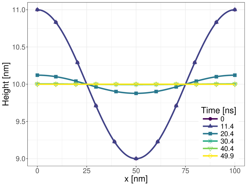

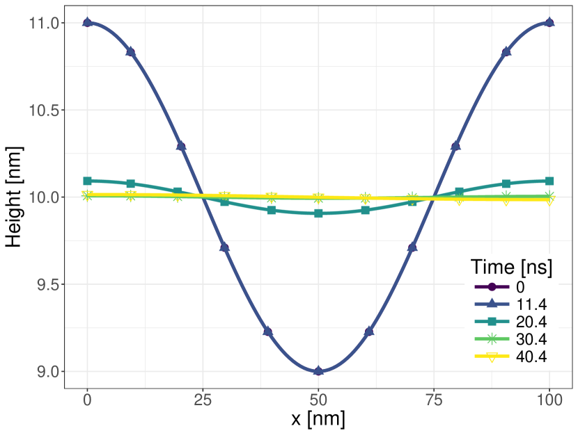
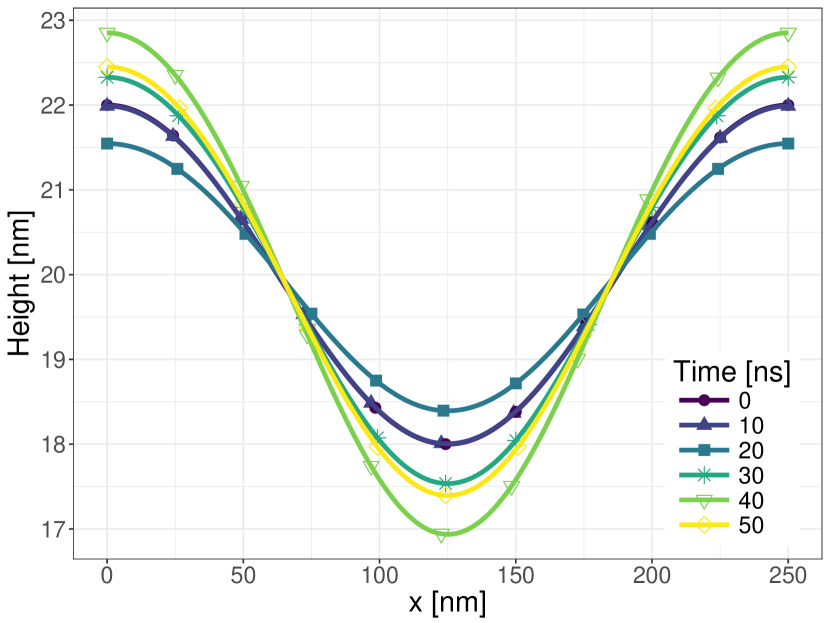
Figure 10 shows the evolution of the interface for a nm film. We use stable perturbation wavelength, nm, that is slightly smaller than the critical one, nm found from the LSA in Section III.1. Hence, we expect the perturbation to be stable. Figure 10(a) shows the evolution of the interface with temperature solution from the reduced model. The perturbation of the interface decays, as expected. Figure 10(b) shows the evolution with the temperature solution from the complete model, where initially (see ns) the perturbation decays, then grows for all following times, and the film eventually breaks into drops. Hence, the two temperature models, which agree for a flat film, produce different evolution for a perturbed interface.
Understanding the difference in stability resulting from the models requires considering both normal and tangential stress balances at the liquid-air interface, that is, both spatial gradients of the surface tension leading to Marangoni effect, and the temporal evolution of surface tension due to the evolution of temperature. We discuss both of these effects next, for both reduced and complete models.
First, let us consider the influence of the temperature on the normal component of the surface force, and ignore the tangential component (therefore ignoring the Marangoni effect). Figure 11 shows the evolution of the interface using the complete model, for (a) constant surface tension, , and (b) temperature dependent, , but the Marangoni effect is not included. In the simulation that use constant surface tension the perturbation is stable, as expected from the dispersion relation, Eq. (35). However, when the surface tension dependence on the temperature is included, the perturbation initially decays (see ns), but grows for all later times. Note in particular that the results shown in Figs. 10(b) and 11(b) are almost identical, showing that the Marangoni effect is essentially irrelevant in the present context. Therefore, the stability change is not due to the spatial variations of , but due to the change of the normal component of the surface tension force due to temporal change of .
We still need to explain why they the results shown in the parts (a) and (b) of Fig. 10 differ. For this purpose, Fig. 12(a) shows the average temperature of the film in the reduced and complete models for the parameters as used in Fig. 10. According to both models, from the melting time at ns, the temperature of the film increases to K, which corresponds to the decrease in the surface tension from to . Figure 12(b) shows the dispersion curve computed using Eq. (35), with and , and . The change in shifts the critical wavenumber, , and the stable perturbation ( which corresponds to ) becomes unstable. This explains why the stable mode in simulations in Figs. 10(b) and 11(b) becomes unstable as the film temperature increases, eventually leading to the film breakup. Note that we have already shown that Marangoni effect is not relevant for the simulations that use the complete model for temperature calculation.
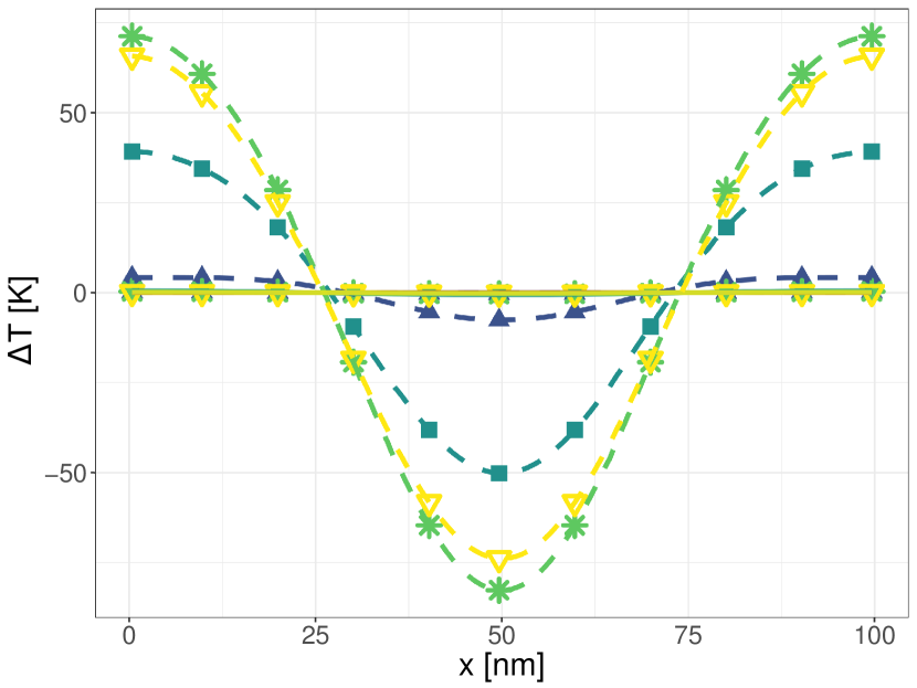
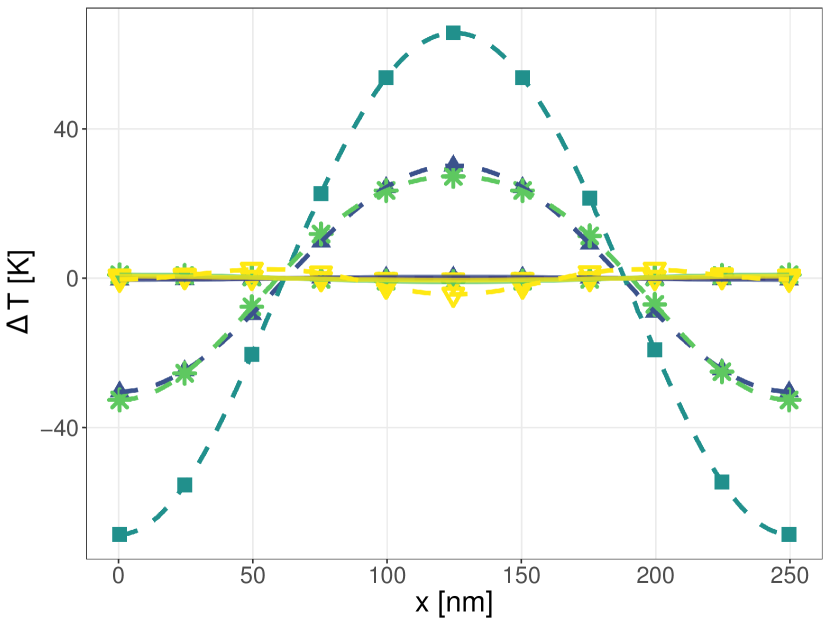
In contrast to the results obtained by implementing the complete temperature model shown in Figs. 10(b) and 11(b), the results obtained with the temperature from the reduced model, Fig. 10(a), show stability, despite the fact that the average temperature of the film increases similarly as in the complete model, see Fig. 12(a). To gain better understanding of this finding, we examine the difference in the temperature solutions along the liquid-air interface for a perturbed stationary film, corresponding to the initial condition used in Figs. 10 and 11. (The motivation for considering a stationary film is the source term dependence on the film thickness - the film evolution would affect the source term, and we prefer to avoid this effect for simplicity of the argument.) Figure 13(a) shows the differences of the computed temperature along the interface from the average temperature. The temperature varies significantly more for the reduced model compared to the complete one. Thus, the temperature gradients at the liquid-air interface are significantly larger for the reduced model, and the stabilizing Marangoni effect prevents the interface in Fig. 10(a) from becoming unstable. This finding explains the different film evolution between the two models.
To summarize the results for the film thickness of nm: If the temperature is computed using the complete model, the Marangoni effect turns out to be irrelevant; however the temporal change of surface tension due to evolving laser pulse and film thickness may influence film stability, leading to instability in the case considered here. If the temperature is computed using the reduced model, then (stabilizing) Marangoni effect may compete with the destabilizing effect of the overall surface tension decrease, leading to stability. Therefore, computing temperature carefully is crucial for understanding the film stability.
III.2.2 Film of Thickness nm;
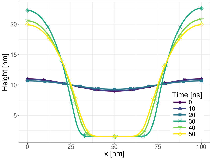
Next, we consider thicker film, with the average thickness of nm. Recall that for nm, the reduced model predicts essentially the opposite direction of the Marangoni effect relative to nm, see Fig. 8. Here we impose a perturbation of the wavelength, nm, which is stable when Marangoni effect is ignored, see the dispersion relation, Eq. (35). Figure 14 shows the comparison of the evolution of the interface using the reduced and complete temperature models. Using the reduced model, Fig. 14(a), we find instability, and the perturbation grows until the film breaks into drops. This is not surprising since the reduced temperature model predicts which destabilizes the film (see Fig. 9(b)). When the temperature is computed using the complete model however, see Fig. 14(b), the evolution is oscillatory: at ns the perturbation decays; at ns and ns the perturbation grows; and at ns the perturbation decays again. Similarly as for nm, to explain these dynamics, we examine the simulations without Marangoni effect, and investigate the influence of the temperature on the normal component of the surface force.
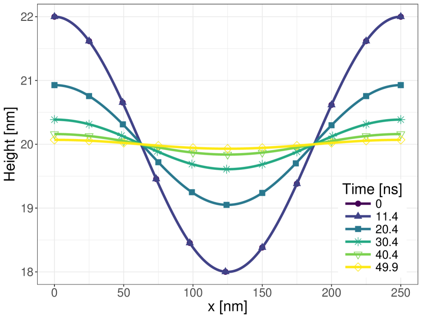
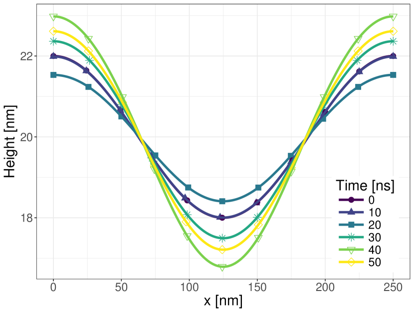
Figure 15 shows the evolution of the interface when the surface tension is (a) constant, , and (b) temperature dependent, , but Marangoni effect is ignored. When constant surface tension is considered, the perturbation is stable, as expected from the LSA. However, for temperature dependent surface tension, we uncover the same dynamics as in Fig. 14(b). Thus, we see again that the Marangoni force is negligible. We show next that the changes in the stability in the complete model are due to the temporal changes of the surface tension.
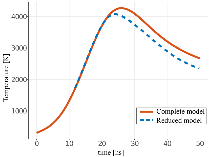
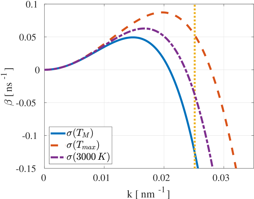
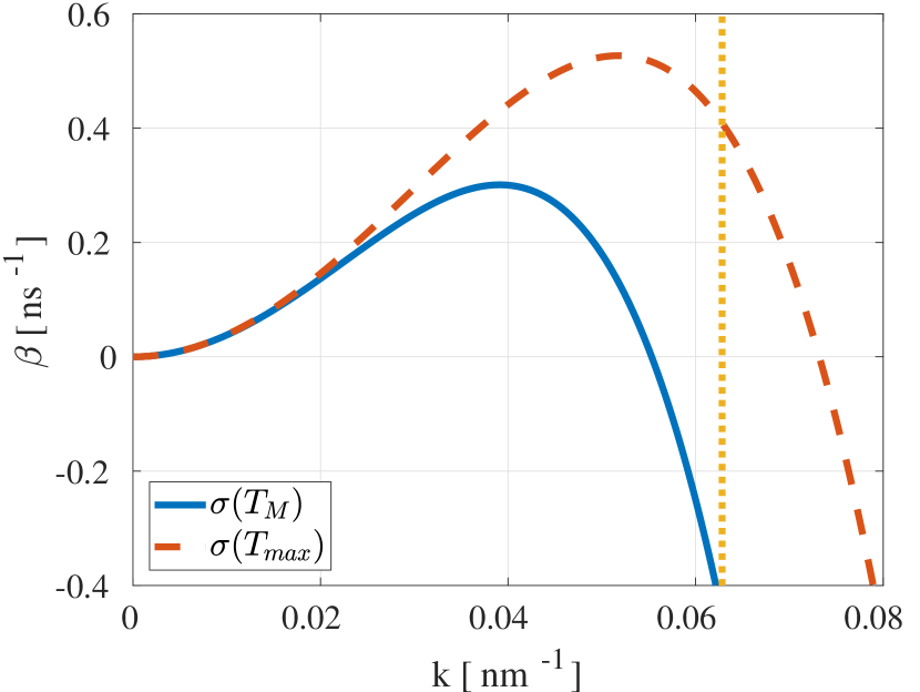
Figure 16(a) shows the average temperature of the film using the reduced and complete models for the parameters as used in Fig. 14. From the melting time, at ns, the temperature evolution (and the surface tension change) are similar as for the nm films. Figure 16(b) shows the dispersion curve computed using Eq. (35), with and , and . The change in shifts the critical wavenumber, , and the (linearly) stable perturbation (nm which corresponds to ) becomes unstable, as we see in Figures 14(b) and 15(b) after ns. After ns, the temperature decreases again to K, hence (see Fig. 16(b)), the perturbation becomes (linarly) stable again. In summary, similarly to the nm film, the stability of the interface using the complete model is governed by the temporal variations of .
Similarly as for the nm film, the temporal changes of the surface tension do not explain the film instability for the temperature from the reduced model in Fig. 14(a). Therefore, we compare again the temperature at the liquid-air interface of a stationary film using the reduced and complete models. Figure 13(b) shows the deviation from the average temperature at the interface of a stationary film corresponding to the initial condition for the simulations shown in Fig. 14. We see once again that the effect of the Marangoni effect is augmented significantly by the reduced model.
To summarize, we find that for both thin and thick films (relative to the critical thickness at which changes sign), the complete and reduced model produce different results, showing clearly that careful computation of heat flow is required to accurately describe the evolution. Using the reduced model, or in other words ignoring the heat conduction in the in-plane direction, leads to qualitatively different results compared to the ones obtained if this assumption is not made.
III.3 The Influence of the Temperature Dependent Viscosity
Here we focus the influence of the viscosity variations with temperature on the stability and breakup dynamics. During the metal heating and melting, the viscosity of the metal changes several orders of magnitude Gale and Totemeier (2003). The viscosity of most metals can be modeled by an exponential as
| (36) |
where and are constants dependent on the material, and is the gas constant Gale and Totemeier (2003).
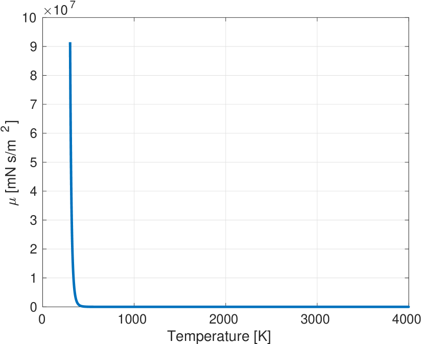
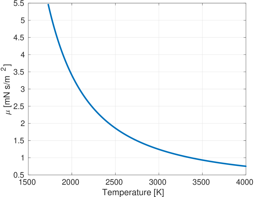
Figure 17 shows the viscosity of nickel as a function of temperature.
The influence of the temperature dependent viscosity on the film breakup can be estimated based on the dispersion relation specified by Eq. (35). This relations says that the stability of the film, and in particular the critical wave number, , do not depend on the viscosity. However, the growth rate, , is inversely proportional to and, as we will see, this may be sufficient to influence the stability.
To study the influence of the variable viscosity on the breakup dynamics, we use the same initial geometry as in Section III.2 within the framework of the complete model described in Section II.1.3. Here, surface tension is taken as temperature dependent, but for simplicity we do not include Marangoni effect (which is essentially irrelevant for the complete model). Figure 18 shows the evolution of the film interface with temperature dependent viscosity compared to the evolution for constant viscosity, . For the nm film, the same evolution dynamics are present in both cases: perturbations initially decay, but start growing as the film temperature rises (see the discussion related to Figs. 10(b) and 11(b)). As expected based on the LSA, the stability of the perturbations is not affected by the variable viscosity, but the growth rate is faster, and therefore the breakup time occurs ns faster with variable viscosity compared to the constant one (see Section III.2). For the nm film, again, the decay and the growth of the perturbations for the variable viscosity follows the same direction as the constant viscosity in Figures 14(b) and 15(b). During the time of the perturbation growth, as in ns to ns for , the perturbation for grows fast enough so that the film breaks. Recall that for , the stability changes after ns, and the film stabilizes due to the decrease of the film temperature. Therefore, inclusion of temperature dependent viscosity can strongly influence the film evolution.

III.4 Discussion of the Influence of Thermal Effects on Film Stability
At the beginning of Section III, we motivated the focus of this work on simple computational domains and initial conditions. In principle, more complex setups would be needed to reach precise understanding regarding the influence of thermal effects in physical experiments where the relevant domains are large and the film and temperature perturbations are more complicated. However, based on the existing results, we are already in the position to develop a basic insight.
To be specific, let us ask for the following question: What is the influence of the fact that the temperature of metal films rises significantly above melting temperature on the film stability? Focusing first on the temperature dependence of surface tension, we start by noting that Marangoni effect is not relevant. However, the overall decrease of surface tension as the temperature of a film raises suggests that shorter wavelengths are expected, see the dispersion curves in Figs. 12(b) and 16(b). Possibly, such an increase of surface tension may be responsible for observation of shorter wavelengths in experiments Trice et al. (2008). Clearly, as the film temperature changes as a function of time due to time-dependent source term (laser pulse) and heat loss through the substrate, the effect of the surface tension change will be time dependent as well. Turning now to temperature dependence of film viscosity, we note that viscosity influences the time scale of instability growth and could therefore influence the film stability strongly, as discussed in Section III.3.
To conclude this brief discussion, a variation of material parameters with temperature clearly influences film stability in a manner which may be complex in particular due to the fact that the relevant time scales, related to the source term and to the temporal evolution of the film itself, are comparable. In general, based on the results presented so far, one expects that heating of the films above melting will result in a decrease of the emerging wavelengths (such as the distance between drops that form eventually), compared to the ones expected if one assumes that the material parameters (surface tension, viscosity) are given by their values at the melting temperature. The details of the instability evolution however may depend on the particular choice of metals, substrates, and laser pulse energy and duration.
III.5 Breakup of Liquid Metal Filaments
In a recent work Hartnett et al. (2017), that included both experimental and computational study, we considered concentration Marangoni effect in a two-metal setup focusing on metal filament geometry. In that study, it was found that concentration Marangoni effect played a significant role. In particular, the Marangoni induced flow led to inversion of instability development, in the sense that initially thicker filament parts (nickel covered by a thin copper film) ended up thinning, while initially thinner filament parts increased in thickness due to concentration induced Marangoni flow. The question that we will consider in the present paper, is whether a similar effect could be observed for thermal Marangoni effect.
To answer this question, we consider the following setup: the initial geometry is a flat filament with superimposed rectangular perturbations (similarly as in Hartnett et al. (2017) just with a single metal (nickel). Since we know from Section III.2 that the temperature gradients are small in the metal film, we increase the thickness of the rectangular perturbations compared to Hartnett et al. (2017) in an attempt to increase the temperature gradients. Therefore we take the base filament thickness as nm, and superimpose the perturbations of nm (so that the film thickness vary between and nm), and the width of the filament is nm. The average filament thickness is kept at nm as in Hartnett et al. (2017). We note that the filament simulations are carried out using the approach described in Hartnett et al. (2017); briefly, we do not consider disjoining pressure here but instead specify the contact angle ( for simplicity), and use Navier-slip boundary condition with the slip length of nm. The simulations consider one half of the perturbation wavelength and half of the filament width, and impose symmetry boundary conditions at all in-plane directions. The fluid is stationary until the melting time of the filament (see Section III.2).
For early times, the initial geometry quickly evolves to a cylindrical filament on a substrate. The basic idea regarding the stability of such a filament could be reached by considering the Rayleigh-Plateau type of instability of a free standing cylindrical jet. Within this model, the growth rate of the perturbations, , is given by Rayleigh (1878); Eggers (1997)
| (37) |
where is the radius of the jet, and and are the modified Bessel functions. Hence the stability of a jet depends on its radius, : the modes, , for which are unstable and the modes for which are stable. Here, is the wavenumber related to the perturbation wavelength, , by . The fastest growing mode corresponds to . In the present context, corresponds to the radius of a filament characterized by the equilibrium contact angle , and of the same cross-sectional area as the initial rectangular geometry of the thickness and width , i.e.,
| (38) |
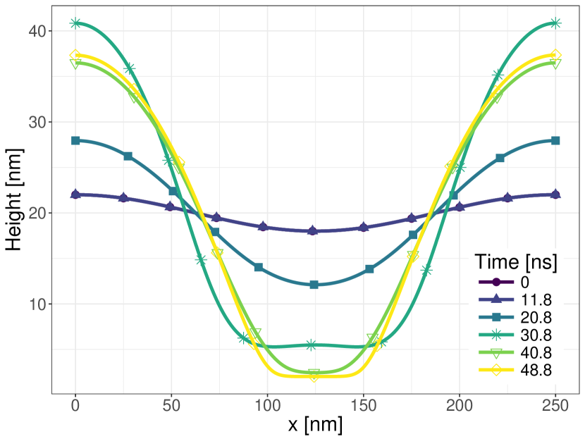
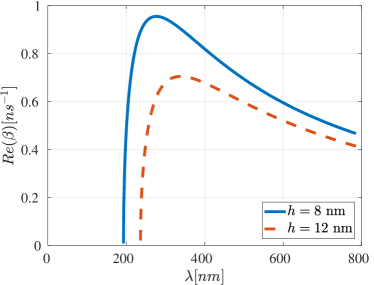
Figure 19 shows the growth rate for a filament. We consider both the filament thickness without the perturbation, nm and the average filament thickness including the perturbations, nm. The Rayliegh-Plateau stability curve gives us an approximation for the critical wavelength, nm using nm; including the presence of substrate is known to make slightly larger Diez et al. (2009b). Our numerical results show consistently that value is in the range nm. In what follows, we show the results for two filaments: one with a stable and one with an unstable perturbation. We compare the results for simulations with and without the thermal effects. The temperature is governed by the complete model described in Section II.1.3.

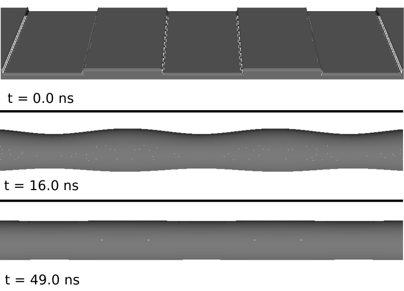
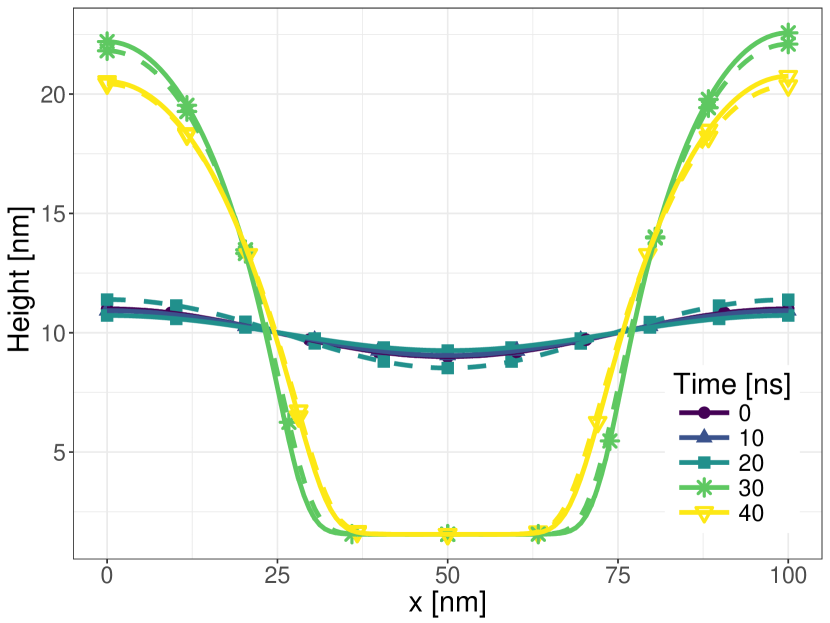
Figure 20 shows the evolution of a linearly stable filament, with the wavelength of the perturbations close to the critical one. The results are similar, independently of whether the surface tension is treated as a constant or temperature dependent. To understand this result, we note that the filament setup differs in a significant manner from the the film one: here, a change of the surface tension does not change the stability of the filament; it only modifies the growth rate. Hence, the thermal variation of the surface tension does not change the qualitative behavior.
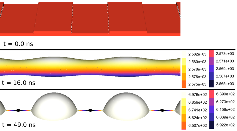
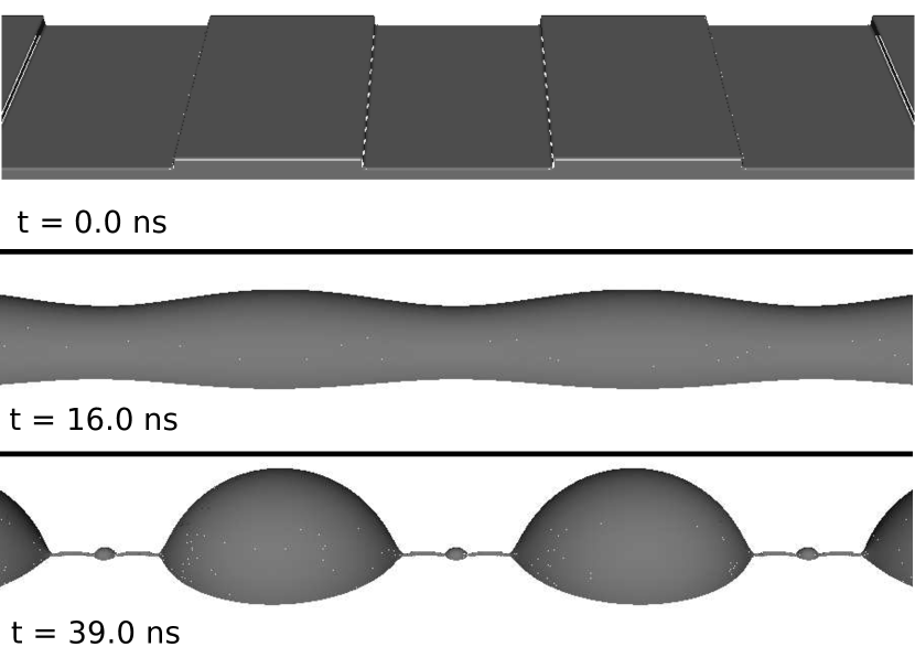
Figure 21 shows the evolution of an unstable filament. Again, the thermocapillary force does not change the qualitative breakup dynamics. However, the breakup with temperature dependent surface tension happens about ns slower compared to the constant surface tension. This is expected, since the increase in the temperature leads to a decrease in the surface tension, which in turn leads to a decrease of the growth rate.
An obvious question to ask is why concentration Marangoni effect, discussed in Hartnett et al. (2017) is so much more prominent compared to the thermal Maranogni effect discussed here. There are at least two sources of the difference: first, the thermal Marangoni effect is much weaker compared to the concentration one (one needs the temperature difference of degrees to produce the change of surface tension of nickel corresponding to the difference of the surface tensions of nickel and copper considered in Hartnett et al. (2017), see Tab. 1): and second, for the setup considered in the present work, the thermal Marangoni effect is induced: the filament needs to heat up for the thermal Marangoni effect to be established; in the setup considered in Hartnett et al. (2017), the concentration Marangoni effect is present from the very beginning of the evolution. We note in passing that the present results also suggest that thermal Marangoni effect can be safely ignored in two (or multi) metal setting: concentration Marangoni effect is expected to play a dominant role.
III.6 Conclusions
In this paper we have studied the influence of the thermal effects on the evolution of thin metal films and filaments. For the films, we have shown that the dynamics of the evolution can change due to the surface tension dependence on temperature. Perhaps surprisingly, the influence of the temperature is not manifested through the Marangoni effect, but through the capillary force (balance of normal stresses). In other words, the thermal effects influence the interface evolution due to the time-dependent changes of the surface tension during a laser pulse.
We have the reached the main conclusion outlined in the preceding paragraph by considering two models for computing the film temperature. The reduced 1D temperature model (Section II.1.1) is found to overestimate the temperature gradients along the free interface, since the in-plane heat conduction is not considered. The complete model, based on the numerical computation of the temperature (Section II.1.3) shows that the temperature gradients along the interface are in fact not strong enough to influence the breakup of the films. The changes in the viscosity during the metal film heating can accelerate the growth of the perturbations, leading to a breakup of films that would not break if a constant value of viscosity at the melting temperature were used. This finding is also to a certain degree unexpected since it is known (at least within the long wave limit) that viscosity influences only the growth rate, and does not modify the range of unstable wave numbers. However, an interplay of the time scales responsible for heating and for instability development modifies the evolution in a nontrivial manner. Our results suggest that the fact that temperature rises significantly over melting will result in the emergence of shorter length-scales compared to the ones expected if the material parameters considered were assumed to be fixed at their values corresponding to the melting temperature.
In the case of filaments, the temperature dependence of surface tension has only rather minor influence on the qualitative behavior of the breakup of the liquid metal filaments. At least for the parameters considered here, the stability of a (single metal) filament is not influenced by surface tension variation. This is in contrast to the two-metal filaments, considered in Hartnett et al. (2017), where concentration dependence of surface tension can qualitatively change the dynamics.
The presented results open new avenues of research. Some of the questions that one may ask are as follows:
-
•
What is the influence of the substrate thickness and thermal properties on the findings reported here? Presumably for sufficiently thin substrate, heat diffusion in the in-plane direction may be less important, modifying the results, and perhaps bringing the findings of the complete model (that includes the heat diffusion in the in-plane direction) and the reduced model (that does not include the in-plane heat diffusion) closer together.
-
•
The result presented here show in some cases oscillatory instability, with the film evolution evolving in a non-monotonous manner. Can one understand the conditions required for such oscillatory evolution more precisely?
-
•
The results of the present paper, combined with the analysis of the propagation of the melting front considered in a stationary setup Font et al. (2017), should allow to analyze evolution of metal films on the substrates that may go through the phase transitions themselves. What is the influence of substrate melting on the film stability?
-
•
How significant are thermal effects for the evolution and stability of multimetal films and alloys?
We expect that the results presented here will serve as a basis for answering some of the outlined questions.
Acknowledgements.
We acknowledge many useful discussions regarding metal films with Ryan Allaire, William Batson III, Linda Cummings, Javier Diez, Francesc Font, Jason Fowlkes, Alejandro Gonzàlez, Kyle Mahady and Philip Rack. This work was supported by the NSF grant No. CBET- 1604351.Appendix A Laser Source Term
The absorption, reflectance and transmittance of a thin metal film can be computed from Maxwell’s equations with appropriate boundary conditions. The equations are greatly simplified when considering a single film layer on a transparent (non-absorbing) substrate. The simplified expressions for computing reflectance and transmittance given in Heavens (1991) are
| (39) | ||||
| (40) |
where the terms in Eqs. (39) and (40) are defined as
and is the metal film thickness, is the wavelength of the incident radiation, is the refractive index of air, and are the metal refractive index and the extinction coefficient respectively, and is the refractive index of the substrate.
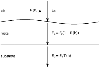
Figure 22 shows a schematic of the laser energy absorption. The incident energy is perpendicular to the film surface. One part of the energy, , is reflected at the film surface, and the rest of the energy, denoted by , penetrates the surface. Then, a part of the laser energy, denoted is transmitted through the metal. Hence the energy absorbed by the metal film is
| (41) |
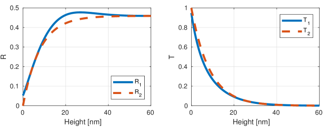
The expressions for and given in Eqs. (39) and (40), can be approximated by simpler functions, as it is done by Trice et al. Trice et al. (2007)
| (42) |
where , and and can be found by fitting and to Eqs. (39) and (40).
Appendix B The Temperature Solution of the Reduced Model in the Limit of Small Film Thickness
The solution to the reduced temperature model given in Section II.1.1 contains integrals that pose numerical difficulties for small film thicknesses. Here we give the expressions that can be used for computing the temperature of the metal film, , and the gradient of the temperature with respect to the film thickness, , to alleviate those difficulties. In the limit of small film thickness, and , can be expanded using asymptotic series as
| (43) |
| (44) |
where
| (45) |
Hence, the integrals in Eqs. (23) and (25) are convergent as . In our simulations, we use the expression given here for small film thicknesses, since the direct evaluation of the integrals in Eqs. (23) and (25) is numerically difficult.
Appendix C Analytical Temperature Solution
Here we provide the details of the analytical temperature solution in the fluid-substrate domain specified in Section II.1.2. Note that in order to simplify the presentation, we change the notation for the domain boundaries compared to Section II.1, and denote the bottom of the substrate as , the fluid-substrate interface as , and the fluid-air interface as . The temperature in the fluid, , and the temperature in the substrate, , satisfy the diffusion equation
| (46) | |||
| (47) |
where
along with the boundary conditions
| (48) | |||||
| (49) | |||||
| (50) | |||||
| (51) |
The source term, is given by Eq. (15). The solution to the above equations can be written compactly in terms of Green’s functions as given in Eqs. (27) and (28), where
| (52) | ||||
| (53) |
Here and are eigenfunctions and eigenvalues computed using separation of variables, and
| (54) | ||||
| (55) | ||||
| (56) |
where , and . In order to simplify the notation, let
| (57) |
The eigenfunctions satisfy the boundary conditions in Eqs. (48) - (51). Hence, it follows
| (58) | ||||
| (59) | ||||
| (60) | ||||
| (61) |
We can solve for the coefficients and using Eqs. (C) and (C)
| (62) | ||||
| (63) |
where
| (64) |
In order to have a solution, we require vanishing determinant of the system of Eqs. (C) - (C)
The equation above leads to the following equation for the eigenvalues,
| (65) |
which can be solved numerically.
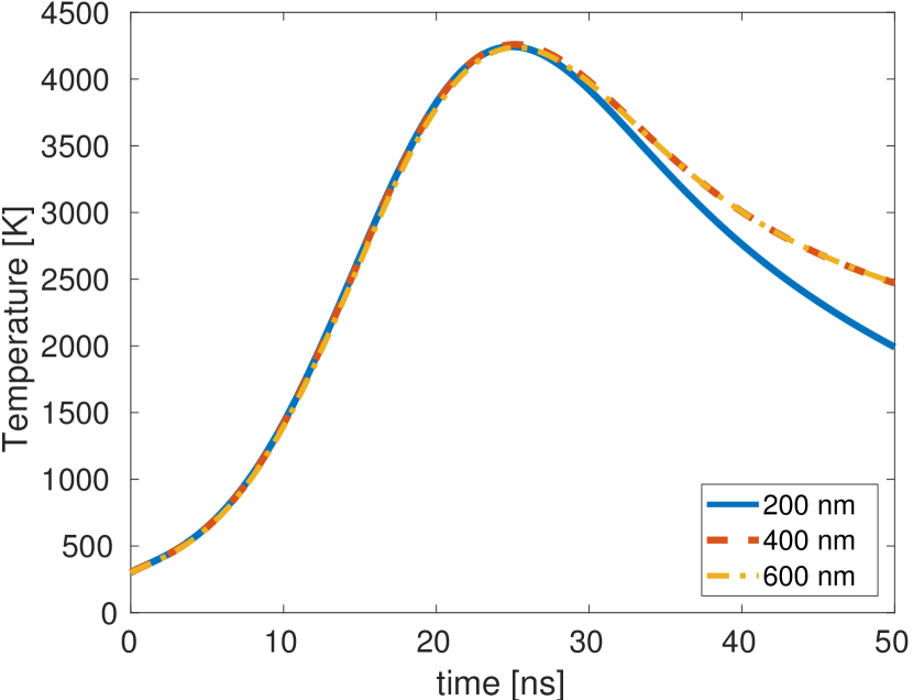
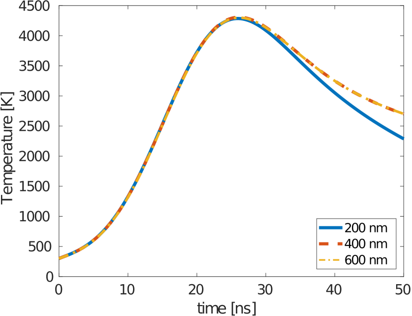
Figure 24 shows the average temperature in the metal as a function of time for different substrate thicknesses. We see that the solution converges as the substrate thickness increases. Hence, for a substrate thick enough, the solution is equivalent to the one obtained in the setup involving semi-infinite substrate. This result is used in Section II.1 to justify comparing the temperature obtained using the reduced model and semi-infinite substrate, with the one obtained by using the complete model and finite substrate thickness.
Appendix D Newton’s Law of Cooling
We show that replacing the continuity of temperature boundary condition at the fluid-substrate interface with Newton’s law of cooling yields an equivalent solution as long as the heat transfer coefficient is large enough.
We replace the boundary condition (49) by
| (66) |
(the notation is the same as in the preceding appendix). Then, the eigenfunctions of the same form as given in Eq. (54) satisfy the boundary conditions (48), (50), (51) and (66). Hence, it follows
| (67) | ||||
| (68) | ||||
| (69) | ||||
| (70) |
From the Eqs. (68) and (D), we can solve for the coefficients and
| (71) | ||||
| (72) |
where
| (73) |
The condition for existence of a solution is vanishing determinant as follows
The equation satisfied by the eigenvalues is now
| (74) |
which can be solved numerically.
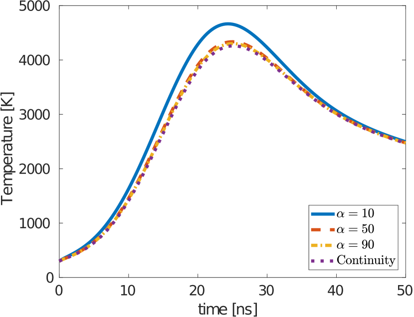
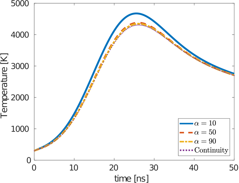
Figure 25 shows the average temperature in the metal as a function of time for different . We see that the solution with Newton’s cooling law converges to the solution with continuity of temperature for large . This result is used in Section II.1 to justify comparing the reduced model that implements continuity of temperature with the complete model that uses Newton’s law of cooling.
References
- Hughes et al. (2017) R. A. Hughes, E. Menumerov, and S. Neretina, “When lithography meets self-assembly: a review of recent advances in the directed assembly of complex metal nanostructures on planar and textured surfaces,” Nanotechnology 28, 282002 (2017).
- Makarov et al. (2016) S. V. Makarov, V. A. Milichko, I. S. Mukhin, I. I. Shishkin, D. A. Zuev, A. M. Mozharov, A. E. Krasnok, and P. A. Belov, “Controllable femtosecond laser-induced dewetting for plasmonic applications,” Laser Photonics Rev. 10, 91 (2016).
- Bischof et al. (1996) J. Bischof, D. Scherer, S. Herminghaus, and P. Leiderer, “Dewetting modes of thin metallic films: Nucleation of holes and spinodal dewetting,” Phys. Rev. Lett. 77, 1536 (1996).
- Ross (2010) F. M. Ross, “Controlling nanowire structures through real time growth studies,” Rep. Prog. Phys. 73, 114501 (2010).
- Favazza et al. (2006) C. Favazza, J. Trice, H. Krishna, and R. Kalyanaraman, “Laser induced short- and long-range orderings of Co nanoparticles on SiO2,” Appl. Phys. Lett. 88, 153118 (2006).
- Xia and Chou (2009) Q. Xia and S.Y. Chou, “The fabrication of periodic metal nanodot arrays through pulsed laser melting induced fragmentation of metal nanogratings,” Nanotech. 20, 285310 (2009).
- Krishna et al. (2010) H. Krishna, R. Sachan, J. Strader, C. Favazza, M. Khenner, and R. Kalyanaraman, “Thickness-dependent spontaneous dewetting morphology of ultrathin Ag films,” Nanotech. 21, 155601 (2010).
- Fowlkes et al. (2014) J. D. Fowlkes, N. A. Roberts, Y. Wu, J. A. Diez, A. G. González, C. Hartnett, K. Mahady, S. Afkhami, L. Kondic, and P. D. Rack, “Hierarchical nanoparticle ensembles synthesized by liquid phase directed self-assembly,” Nano Letters 14, 774 (2014).
- Reinhardt et al. (2013) H. Reinhardt, H-C. Kim, and C. Pietzonka, “Self-organization of multifunctional surfaces - the fingerprints on a complex system,” Advanced Mat. 25, 3313 (2013).
- Kondic et al. (2009) L. Kondic, J. A. Diez, P. D. Rack, Y. Guan, and J. D. Fowlkes, “Nanoparticle assembly via the dewetting of patterned thin metal lines: Understanding the instability mechanisms,” Phys. Rev. E. 79, 1 (2009).
- Gonzalez et al. (2013a) A. G. Gonzalez, J. D. Diez, Y. Wu, J.D. Fowlkes, P. D. Rack, and L. Kondic, “Instability of Liquid Cu Films on a SiO2 Substrate,” Langmuir 13, 9378 (2013a).
- Gonzalez et al. (2013b) A. G. Gonzalez, J. D. Diez, and L. Kondic, “Stability of a liquid ring on a substrate,” J. Fluid Mech. 718, 213 (2013b).
- Kondic et al. (2015) L. Kondic, N. Dong, Y. Wu, J. D. Fowlkes, and P. D. Rack, “Instabilities of nanoscale patterned metal films,” EPJST 224, 369 (2015).
- Mahady et al. (2016) K. Mahady, S. Afkhami, and L. Kondic, “A numerical approach for the direct computation of flows including fluid-solid interaction: Modeling contact angle, film rupture, and dewetting,” Phys. Fluids 28, 062002 (2016).
- Mahady et al. (2015a) K. Mahady, S. Afkhami, and L. Kondic, “A volume of fluid method for simulating fluid/fluid interfaces in contact with solid boundaries,” J. Comput. Phys. 294, 243 (2015a).
- Mahady et al. (2015b) K. Mahady, S. Afkhami, and L. Kondic, “On the influence of initial geometry on the evolution of fluid filaments,” Phys. Fluids 27, 092104 (2015b).
- Diez et al. (2009a) J. Diez, A. González, and L. Kondic, “On the breakup of fluid rivulets,” Phys. Fluids 21, 082105 (2009a).
- Trice et al. (2007) J. Trice, D. Thomas, C. Favazza, R. Sureshkumar, and R. Kalyanaraman, “Pulsed-laser-induced dewetting in nanoscopic metal films: Theory and experiments,” Phys. Rev. B 75, 235439 (2007).
- Trice et al. (2008) J. Trice, D. Thomas, C. Favazza, R. Sureshkumar, and R. Kalyanaraman, “Novel Self-Organization Mechanism in Ultrathin Liquid Films: Theory and Experiment,” Phys. Rev. Lett. 101, 017802 (2008).
- Atena and Khenner (2009) A. Atena and M. Khenner, “Thermocapillary effects in driven dewetting and self assembly of pulsed-laser-irradiated metallic films,” Phys. Rev. B 80, 075402 (2009).
- Dong and Kondic (2016) N. Dong and L. Kondic, “Instability of nanometric fluid films on a thermally conductive substrate,” Phys. Rev. Fluids 1, 063901 (2016).
- Seric et al. (2017) I. Seric, S. Afkhami, and L. Kondic, “Direct numerical simulation of variable surface tension flows using a Volume-of-Fluid method,” to appear: J. Comput. Phys. (2017).
- Font et al. (2017) F. Font, S. Afkhami, and L. Kondic, “Substrate melting during laser heating of nanoscale metal films,” Int. J. Heat Mass Transfer 113, 237 (2017).
- Brackbill et al. (1992a) J. U. Brackbill, D. B. Kothe, and C. Zemach, “A continuum method for modeling surface tension,” J. Comput. Phys. 100, 335 (1992a).
- Francois et al. (2006) M. M. Francois, S. J. Cummins, E. D. Dendy, D. B. Kothe, J. M. Sicilian, and M. W. Williams, “A balanced-force algorithm for continuous and sharp interfacial surface tension models within a volume tracking framework,” J. Comput. Phys. 213, 141 (2006).
- Afkhami and Bussmann (2009) S. Afkhami and M. Bussmann, “Height functions for applying contact angles to 3D VOF simulations,” Int. J. Numer. Meth. Fluids 61, 827 (2009).
- Popinet (2009) S. Popinet, “An accurate adaptive solver for surface-tension-driven interfacial flows,” J. Comput. Phys. 228, 5838 (2009).
- Landau and Lifshitz (1987) L. D. Landau and E. M. Lifshitz, Fluid mechanics, 2nd, Vol. 6 (Pergamon Press, Oxford, 1987).
- Levich and Krylov (1969) V. G. Levich and V. S. Krylov, “Surface-tension-driven phenomena,” Annu. Rev. Fluid Mech. 1, 293 (1969).
- Brackbill et al. (1992b) J. U. Brackbill, D. B. Kothe, and C. Zemach, “A continuum method for modeling surface tension,” J. Comput. Phys. 100, 335 (1992b).
- Ajaev and Willis (2003) V. S. Ajaev and D. A. Willis, “Thermocapillary flow and rupture in films of molten metal on a substrate,” Phys. Fluids 15, 3144 (2003).
- Heavens (1991) O. S. Heavens, Optical properties of thin solid films (New York: Dover Publications, 1991).
- Gale and Totemeier (2003) W. F. Gale and T. C. Totemeier, Smithells metals reference book (Butterworth-Heinemann, 2003).
- Hartnett et al. (2017) C. A. Hartnett, I. Seric, K. Mahady, L. Kondic, S. Afkhami, J. D. Fowlkes, and P. D. Rack, “Exploiting the Marangoni effect to initiate instabilities and direct the assembly of liquid metal filaments,” Langmuir 33, 8123 (2017).
- Francois and Swartz (2010) M. M. Francois and B. K. Swartz, “Interface curvature via volume fractions, heights, and mean values on nonuniform rectangular grids,” J. Comput. Phys. 229, 527 (2010).
- Özışık (1989) M. Necati Özışık, Boundary value problems of heat conduction (Dover Publications, 1989).
- Popinet (2013-12-06) S. Popinet, “Gerris Flow Solver,” , http://gfs.sourceforge.net/wiki/index.php (2013-12-06).
- Oron et al. (1997) A. Oron, S. H. Davis, and S. G. Bankoff, “Long-scale evolution of thin liquid films,” Rev. Mod. Phys. 69, 931 (1997).
- Diez and Kondic (2007) J. A. Diez and L. Kondic, “On the breakup of fluid films of finite and infinite extent,” Phys. Fluids 19, 072107 (2007).
- Rayleigh (1878) L. Rayleigh, “On the instability of jets,” Proc. London Math. Soc. 1, 4 (1878).
- Eggers (1997) J. Eggers, “Nonlinear dynamics and breakup of free-surface flows,” Rev. Mod. Phys. 69, 865 (1997).
- Diez et al. (2009b) J. A. Diez, A. G. Gonzalez, and L. Kondic, “On the breakup of fluid rivulets,” Phys. Fluids 21 (2009b).
- Johnson and Christy (1974) P. B. Johnson and R. W. Christy, “Optical constants of transition metals: Ti, V, Cr, Mn, Fe, Co, Ni, and Pd,” Phys. Rev. B 9, 5056 (1974).