Coherifying quantum channels
Abstract
Is it always possible to explain random stochastic transitions between states of a finite-dimensional system as arising from the deterministic quantum evolution of the system? If not, then what is the minimal amount of randomness required by quantum theory to explain a given stochastic process? Here, we address this problem by studying possible coherifications of a quantum channel , i.e., we look for channels that induce the same classical transitions , but are “more coherent”. To quantify the coherence of a channel we measure the coherence of the corresponding Jamiołkowski state . We show that the classical transition matrix can be coherified to reversible unitary dynamics if and only if is unistochastic. Otherwise the Jamiołkowski state of the optimally coherified channel is mixed, and the dynamics must necessarily be irreversible. To assess the extent to which an optimal process is indeterministic we find explicit bounds on the entropy and purity of , and relate the latter to the unitarity of . We also find optimal coherifications for several classes of channels, including all one-qubit channels. Finally, we provide a non-optimal coherification procedure that works for an arbitrary channel and reduces its rank (the minimal number of required Kraus operators) from to .
I Introduction
Random processes are ubiquitous in both classical and quantum physics. However, the nature of randomness in these two regimes differs significantly. On the one hand, classical random evolution is necessarily irreversible. On the other hand, quantum evolution may be completely deterministic (and thus reversible if no measurement is performed), but nevertheless lead to random measurement outcomes of observable by transforming a system into a coherent superposition of eigenstates of . When probing the dynamics of the system one can therefore observe the same random transitions, irrespectively of whether the evolution is coherent or incoherent. The question then arises: to what extent an observed random transformation can be explained via the underlying deterministic and coherent process, and how much unavoidable classical randomness must be involved in it?
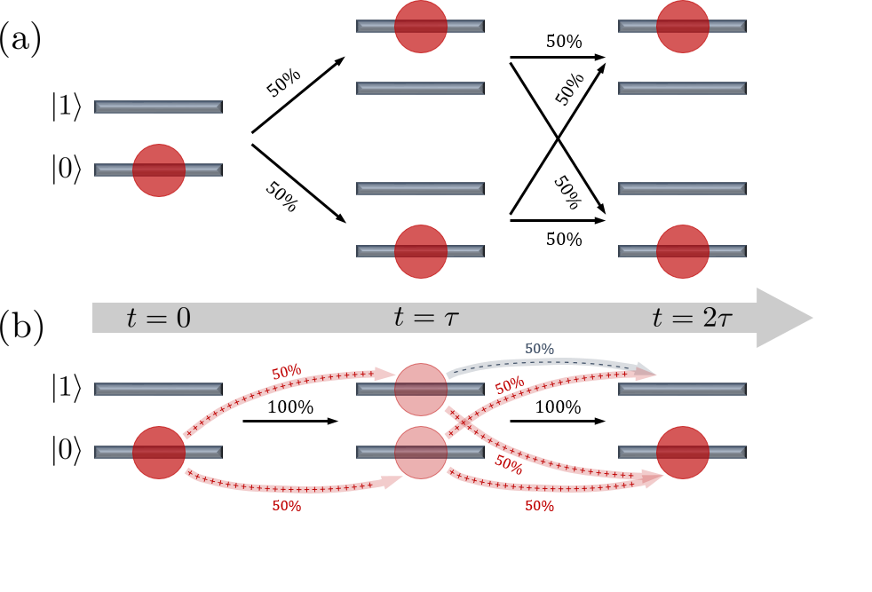
To formulate this problem more precisely, consider a -dimensional physical system undergoing some unknown evolution. In order to characterize it, one first measures the system, finding it in some well-defined state , e.g., an eigenstate of observable . One then allows the system to evolve for time and performs the same measurement again, this time finding the system in state . By repeating this procedure many times and collecting the statistics of measurement outcomes, one can reconstruct the transition matrix , with entries describing transition probabilities between states and . Now, for a truly random classical process, repeating it (e.g., by letting the system evolve for instead of ) leads to the evolution described by . We illustrate this in Fig. 1a for an exemplary two-dimensional system. However, in quantum physics, different transitions (paths) of can interfere with each other, so that the composition of two processes will generally not be described by a transition matrix . In particular, the compound process can even become fully deterministic, leading to the complete disappearance of the observed randomness (see Fig. 1b). Our question can then be rephrased as: what is the optimal coherification of the random process described by a classical transition matrix ?
A more formal motivation for our studies comes from the resource-theoretic approach to quantum information. To explain it, let us first consider a simpler and better-known problem: how coherent is a given quantum state of a -dimensional system, and to what extent can it be transformed into a “more coherent” state? Note that we do not refer here to the notion of spin-coherent states, which does not depend on the choice of basis Zhang et al. (1990), but rather to a more recent concept of coherence with respect to a given basis Baumgratz et al. (2014), distinguished for instance by the eigenbasis of the system’s Hamiltonian. Any state represented by a density matrix that is diagonal in the preferred basis is incoherent in that sense, as it corresponds to a statistical mixture of classical states. On the other hand, a quantum state whose non-diagonal elements, called coherences, do not vanish may lead to non-classical effects of quantum interference. However, a generic system-environment interaction leads to the process of decoherence, due to which the off-diagonal entries tend to zero and the state becomes classical.
From the perspective of emerging quantum information technologies, coherence can be treated as a resource Brandão and Gour (2015) allowing one to perform tasks impossible otherwise. It is then crucial to assess which quantum states are more valuable, i.e., have more coherence. One is thus confronted with the problem of quantifying coherence Baumgratz et al. (2014), which effectively means ordering the set of quantum states according to their coherence properties. Several competing measures of coherence of a quantum state were recently discussed in the literature, e.g., the norm of the off-diagonal entries of a density matrix or the relative entropy between a state and its decohered version (for a comprehensive review see Ref. Streltsov et al. (2016) and references therein). Note that the diagonal density matrices, appearing as a result of the process of decoherence, are situated at the very bottom of this ordering, as they are classical and do not carry any coherence at all.
The problem of quantifying coherence has been taken a step farther by focusing on cohering power of quantum channels Mani and Karimipour (2015), i.e., studying the degree to which a quantum map can create coherence in an initially incoherent state. One can analyze the maximal or the average gain of coherence, where the average is taken over a suitable set of incoherent states. Such an approach is applicable to unitary transformations García-Díaz et al. (2016); Zanardi et al. (2017a) and to non-unitary operations Zanardi et al. (2017b); Xi et al. ; Bu et al. (2017), and in this way quantum channels can be ordered depending on their power to create coherence.
Within this approach, however, quantum states and their coherence are still the central objects of interest. Here, we take an alternative path and make quantum channels themselves the main focus of our study. Employing the well known Jamiołkowski–Choi isomorphism Jamiołkowski (1972); Choi (1975), i.e., the fact that every quantum channel is isomorphic to a bipartite quantum state Życzkowski and Bengtsson (2004), we propose to apply the measures of coherence to bipartite states associated with a given channel. This way we can quantitatively investigate the problem posed at the beginning of this section: how coherent can a given random transformation be? More precisely, for a given stochastic transition matrix we look for the maximally coherent quantum channel , which under complete decoherence collapses to , so that the diagonal parts of both Jamiołkowski states are equal. We first prove that a channel whose classical action is described by a transition matrix can be coherified to a reversible unitary transformation if and only if is unistochastic. We then derive general upper and lower bounds on the optimal coherification of a channel described by a non-unistochastic . Finally, we construct optimally coherified maps for any one-qubit channel and certain classes of channels acting on higher dimensional systems.
The paper is organized as follows. In Sec. II we set the scene by introducing necessary concepts concerning the coherence and mixedness of quantum states and channels, and formulate the optimal coherification problem. General limitations for coherifying quantum channels are then derived and analyzed in Sec. III, where we also study particular families of maps in detail. In Sec. IV we discuss physical interpretation of coherence and purity of a channel, and relate these quantities to unitarity Wallman et al. (2015) and cohering power Mani and Karimipour (2015). Concluding remarks are presented in the final Sec. V, while some technical results, predominantly concerning channels acting on two- and three-dimensional spaces, are relegated to Appendices A-D.
II Setting the scene
II.1 Coherence and mixedness of quantum states
A state of a finite-dimensional quantum system is described by a density operator acting on a -dimensional Hilbert space that is positive, , and normalized by a trace condition, . The convex set of all density matrices of size , denoted by , has dimensions and contains the -dimensional simplex of normalized probability vectors of length . By we will denote the probability vector with entries given by the eigenvalues of arranged in a non-increasing order.
A state is pure if (equivalently if ), so it can be represented by a -dimensional projector, ; and mixed otherwise. Typical measures used to quantify the degree of mixedness of a given state Nielsen and Chuang (2010); Bengtsson and Życzkowski (2017) include the von Neumann entropy,111Within this work we will use to denote both the von Neumann entropy of a density matrix, as well as the Shannon entropy of a probability distribution.
| (1a) | |||
| and purity, | |||
| (1b) | |||
Note that, since the above measures are directly related to the eigenvalues of , they are unitarily-invariant, and thus the mixedness of a quantum state is preserved under unitary dynamics.
On the other hand, in order to study coherence of one first needs to specify a basis with respect to which the coherence is measured Baumgratz et al. (2014). This basis may be distinguished by the problem under study, e.g., within quantum thermodynamics one is mainly concerned with superposition of energy eigenstates Lostaglio et al. (2015a, b). Here, however, we will study the problem in a general quantum information context, and thus we will simply fix an orthonormal basis . We say that a state is incoherent, or classical, when it is diagonal in the chosen basis. Classical states can be alternatively represented by a probability distribution , where denotes a mapping of a density matrix into a probability vector with . With a slight abuse of the notation we will also write if is diagonal. Before we introduce measures of coherence, let us first define a completely decohering quantum channel ,
| (2) |
Note that under the action of any quantum state undergoes complete decoherence and becomes diagonal in the preferred basis. Thus, and the associated probability distribution can be considered as the classical version of a general quantum state . Notice also that is a projector onto as and for all .
The problem of quantifying the amount of coherence present in a state has been addressed in Ref. Baumgratz et al. (2014), while an earlier work Åberg (2006) was devoted to quantifying quantum superposition. Two particular measures of coherence that we will focus on in this work are the relative entropy of coherence,
|
|
(3a) | ||
| and the -norm of coherence222We note that from the resource-theoretic perspective Baumgratz et al. (2014) does not strictly satisfy all desirable requirements for a coherence measure. While it is true that under incoherent CPTP maps the -norm of coherence is non-increasing, it can increase on average under selective measurements. However, in our study of coherence of quantum channels, the resource-theoretic constraints have no clear physical meaning, and thus is a completely legitimate measure of coherence. | |||
|
|
(3b) | ||
It is evident that the measures of coherence are directly related to the measures of mixedness. More precisely, the relative entropy of coherence is the difference between the entropy of a classical version of a state and the quantum state itself; and the -norm of coherence is the difference between the purity of a quantum state and the purity of its classical version.
Among the family of states with a fixed spectrum, i.e., belonging to a unitary orbit, the measures of mixedness are equal, but the measures of coherence vary significantly. The minimal coherence, equal to zero, is obtained for the diagonal state , where is the unitary matrix containing the eigenvectors of . The maximal coherence is achieved by the contradiagonal state Lakshminarayan et al. (2014), , where is a Fourier matrix (or, more generally, a complex Hadamard matrix Tadej and Życzkowski (2006)), which is unitary and has entries with the same modulus, . Since all diagonal elements of the contradiagonal state are equal, , one gets and .
On the other hand, among the family of states with a fixed diagonal, i.e., quantum states that under the action of decohere to the same classical state, both mixedness and coherence measures vary. However, they are maximized and minimized by the same states, which can be directly inferred from Eqs. (3a)-(3b). The minimum can be obtained by acting with the decohering channel (that leaves the diagonal unchanged) on any member of the family, leading to zero coherence. In a similar fashion we can define an optimal coherifying transformation (which should not be confused with coherence measures) that maps any member of the family into a state that maximizes purity (and thus coherence),
| (4) |
This problem has a simple solution for any mixed state . Identifying its diagonal elements with components of a probability vector , one can write explicitly a family of optimally coherifying transformations
| (5) |
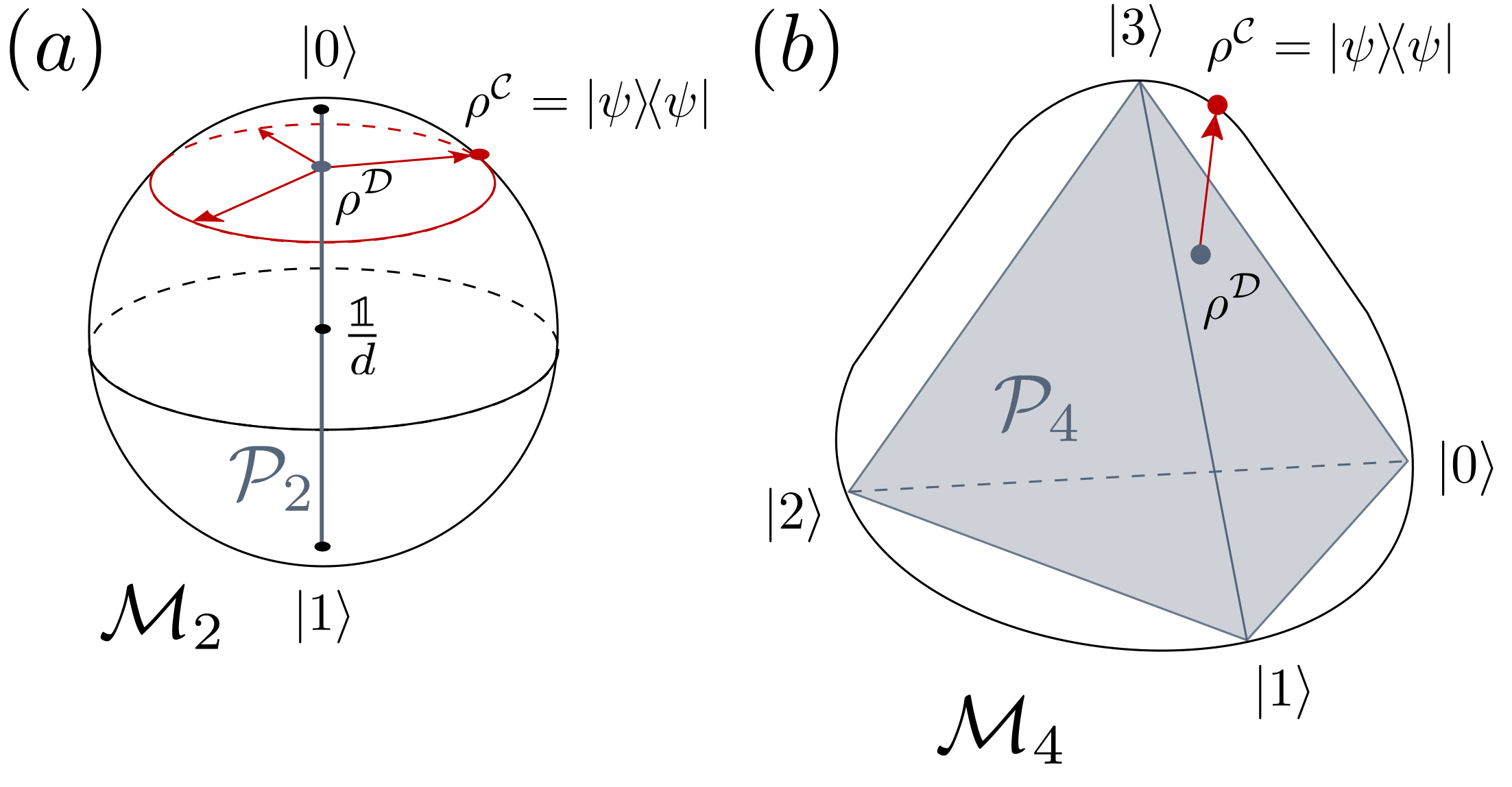
where the phases, , are arbitrary. The mixedness of such coherified states is zero and coherence achieves its maximal value, and . In our work we will also refer to non-optimal coherification transformations that map a diagonal state into a state with the same diagonal but some non-zero off-diagonal terms. In Fig. 2 we illustrate the ideas of decoherence and coherification of quantum states using low-dimensional examples.
Let us emphasize that Eq. (4) does not describe a realistic physical process, but rather it provides an answer to a legitimate question concerning the possible past of an irreversible quantum dynamics. Such a fictitious coherification can be treated as a kind of a formal inverse of the process of decoherence. More precisely, for a diagonal state we have ; and for a pure state we have , where the equivalence is up to phase factors of the off-diagonal terms.
Finally, note that coherification can be compared to the known procedure Nielsen and Chuang (2010); Kleinmann et al. (2006) of purification of a quantum state. Any mixed quantum state can be purified at the expense of increasing the dimension of the Hilbert space. More precisely, for any state its purification is given by a pure state of the extended system, such that its partial trace reads . The Schmidt vector of coincides with the spectrum of , e.g., if the state is maximally mixed, the state is maximally entangled. Both formal procedures are not unique and they allow one to find possible preimages of with respect to non-invertible physical operations. Namely, purification yields states of an extended system which are transformed into by a partial trace; and coherification of a state provides states of the same size which decay into due to decoherence.
II.2 Coherence and mixedness of quantum channels
In this work we generalize the notion of coherence and mixedness of quantum states to quantum channels, i.e., completely positive trace preserving (CPTP) maps acting on density matrices of order . We will denote by the set of all quantum channels, also called stochastic maps, acting on . Recall that for any one can define the associated Jamiołkowski state Jamiołkowski (1972), as the image of the extended map acting on a maximally entangled state,
| (6) |
with and denoting the identity channel. Note also that the Jamiołkowski state is proportional to the dynamical matrix of Choi Choi (1975), so that . Here, with a slight abuse of the notation, denotes the representation of the channel as a matrix of size , i.e., a superoperator with entries in the preferred basis given by ; and the reshuffling transformation, , exchanges elements of a matrix in such a way that square blocks of size after reshaping form rows of length , so that – see Ref. Życzkowski and Bengtsson (2004) for further details. Finally, for every quantum channel there exists a Kraus decomposition Nielsen and Chuang (2010), or the operator-sum representation, of the form
| (7) |
where are called Kraus operators. Due to trace preserving condition these satisfy , where denotes the identity matrix of size .
The condition of is equivalent to Jamiołkowski (1972)
| (8a) | |||||
| (8b) | |||||
These conditions imply that diagonal elements (in the preferred basis) of the Jamiołkowski state correspond to the entries of a (column-stochastic) transition matrix ,
| (9) |
with and . The set of stochastic transition matrices of order will be denoted by . This set of classical maps has dimensions and can be embedded inside the set of quantum maps with dimensions Bengtsson and Życzkowski (2017). Since the diagonal of (up to a constant factor) is given by the elements of a transition matrix , we will write , where denotes the (row-wise) vectorization of a matrix,
| (10) |
which can be also written as
| (11) |
with denoting a transpose. We also define by the Hermitian conjugate of the right hand side of Eq. (10).
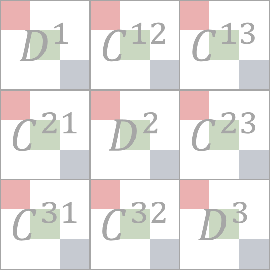
Before we define the coherence of a quantum channel , let us first physically interpret the entries of the corresponding Jamiołkowski state . Writing it in the matrix form in the distinguished basis we have the following block form
| (12) |
with
|
|
(13) |
where and formally . We thus see that the diagonal elements of describe how initial populations (occupations in the preferred basis) affect the final population of a state ; and the off-diagonal elements of describe how initial coherences affect the final population of a state . On the other hand, the diagonal elements of describe how initial populations affect the final coherence between states and ; and the off-diagonal elements of describe how initial coherences affect the final coherence between states and .
In analogy with the standard completely decohering map, Eq. (2), we also define a decohering operation which acts on any quantum channels by bringing its corresponding Jamiołkowski state into the diagonal form,
| (14) |
Diagonal Jamiołkowski state represents the classical map acting on probability vectors of size . The action of on any state is first to completely decohere it into , and then to transform the probability vector into , so that the final state is always classical. Therefore, again with a slight abuse of the notation, we will write and if is diagonal and .
As every quantum channel is isomorphic to a density matrix on an extended Hilbert space, , it is then natural to apply the standard measures of mixedness and coherence to the Jamiołkowski state and to characterize in this way the properties of the associated channel. More formally, for any quantum channel acting on quantum states of size one defines the entropy of a channel Roga et al. (2011),
| (15a) | |||
| and the purity of a channel, | |||
| (15b) | |||
These quantities allow us to introduce
-
1.
entropic coherence of a channel,
(16a) and
-
2.
-norm coherence of a channel,
(16b)
Note that can be decomposed into two terms,
| (17) |
with measuring coherence coming from diagonal blocks and from off-diagonal blocks , i.e.,
| (18) |
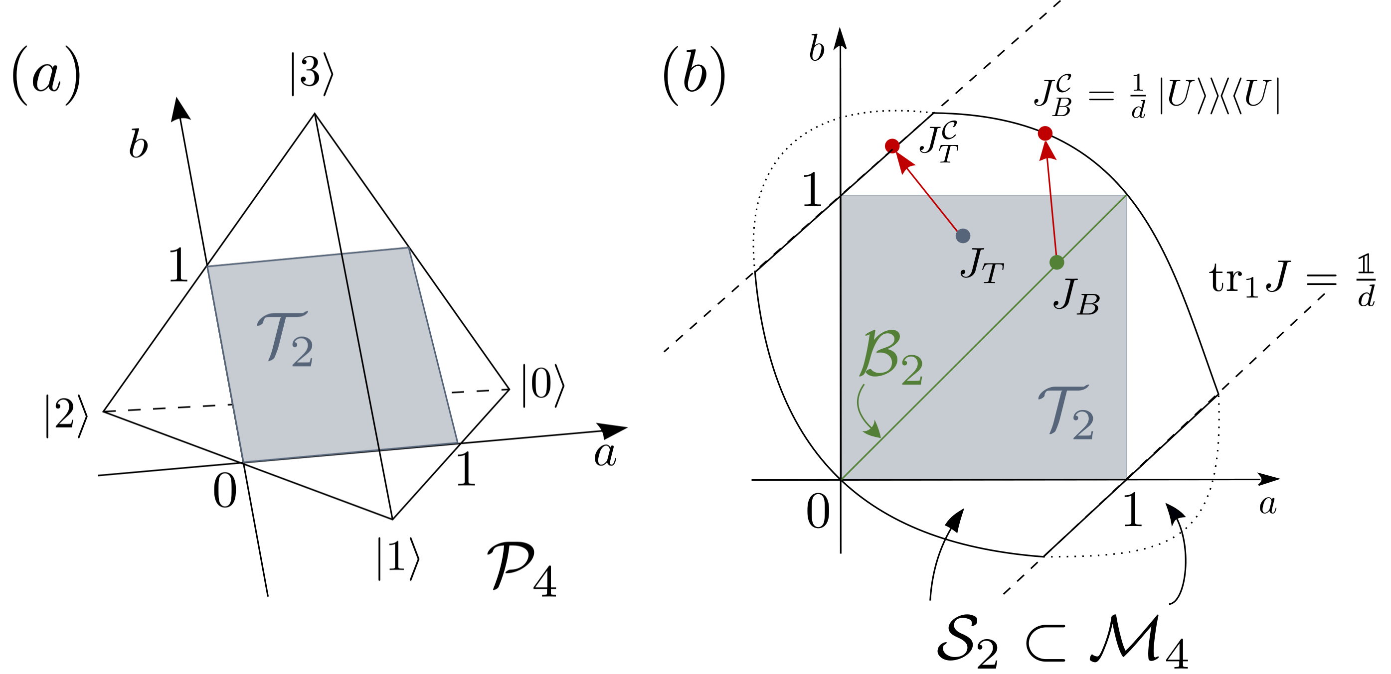
We now arrive at the central technical problem analyzed in the current work: coherifying quantum channels. Note that, given a fixed diagonal, , of the Jamiołkowski state (equivalently: a transition matrix specifying the classical action of , i.e., ), one can always find the corresponding coherified pure state by simply employing the optimal coherification recipe, Eq. (5). In general, however, such a pure state will not satisfy the trace preserving condition, Eq. (8b). More precisely, this condition is equivalent to , and thus the choice of the off-diagonal elements of (describing the effect of initial coherences on final populations) is constrained beyond the standard positivity constraint. Hence, for any classical map represented by a stochastic matrix it is legitimate to ask the following question: what is the corresponding optimally coherified quantum map with the same classical part, such that its coherence is the largest (or its mixedness is the smallest). In Fig. 3 we illustrate the ideas of decoherence and coherification of quantum channels using one-qubit maps as an example.
III Limitations of coherifying quantum channels
In this section we will investigate the limits to which a given quantum channel , with a prescribed classical action , can be coherified into an optimal channel with minimal entropy or maximal purity. To characterize potential coherification of a given channel we will simply use both coherence measures introduced above in Eqs. (16a) and (2). We thus first define optimally coherified channels according to both measures,
| (19a) | |||||
| (19b) | |||||
which allows us to define
-
1.
entropic coherification,
(20a) and
-
2.
-norm coherification,
(20b)
We will be particularly interested in the extremal case when the coherified channel is classical, . Then, since , we have
| (21a) | ||||
| (21b) | ||||
Note that, although we introduced two potentially inequivalent coherification procedures, and (with corresponding Jamiołkowski states and ), while deriving general bounds affecting both maximization processes, we will simply use (and ).
We now need to point out an important relation linking the classical action of a channel and its Kraus decomposition. Namely, for a channel with a classical action , the Kraus decomposition of , defined in Eq. (7), satisfies
| (22) |
with denoting the entry-wise product (also known as Hadamard or Schur product) and being the complex conjugate of .
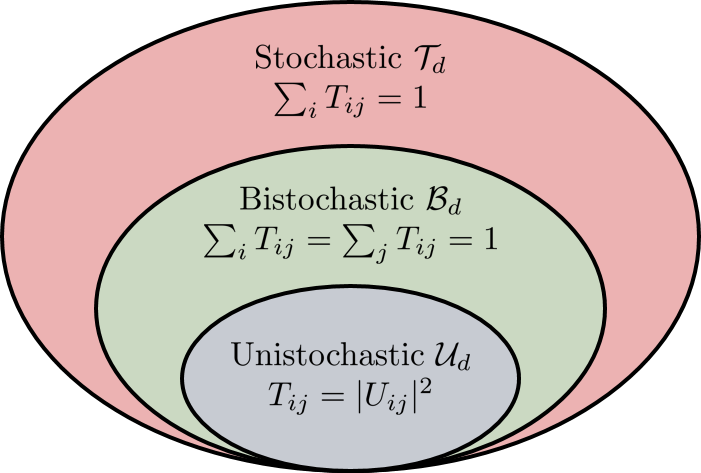
The problem of optimal coherification of a channel naturally splits into three cases, corresponding to three families of transition matrices presented in Fig. 4. The biggest family, , consists of all stochastic matrices of size , i.e., the most general transformations mapping the set of -dimensional probability vectors into itself. These are defined by and . The second family, , is given by the set of bistochastic matrices, which in addition to being stochastic satisfy . This additional condition encodes the fact that bistochastic matrices map the uniform distribution, , into itself. The third analyzed case corresponds to unistochastic matrices , which are such bistochastic matrices whose entries can be written as , for some unitary matrix . Note that this condition, using Eq. (22), can alternatively be written as . While bistochastic matrices form a proper subset of stochastic matrices for all , the unistochastic matrices form a proper subset of bistochastic matrices only for , as every bistochastic matrix of order is unistochastic. Interestingly, the exact boundary of the set of unistochastic matrices is known only for Dunkl and Życzkowski (2009), while for the set of unistochastic matrices is not convex Bengtsson et al. (2005).
III.1 Unistochastic matrices and unitary channels
We start our analysis from the smallest family of unistochastic matrices. We will thus consider optimal coherification of a channel for which . We say that a given channel can be completely coherified if there exists that is pure, has the same diagonal as and still corresponds to a valid channel. From Eq. (6) it is clear that the Jamiołkowski state is pure if and only if the corresponding map is unitary. This simple observation can then be formalized as follows:
Proposition 1.
A quantum channel , with the corresponding Jamiołkowski state , can be completely coherified to a unitary transformation if and only if its classical action is given by a unistochastic matrix.
Proof.
First assume that can be completely coherified. This means that there exists a pure state with , and that it corresponds to a valid channel . However, pure Jamiołkowski states correspond to unitary channels, so that [comparing Eq. (6) and Eq. (10)]
| (23) |
Therefore, the diagonal of (and, by assumption, of ) is given by , which corresponds to a unistochastic matrix. Conversely, assume that the diagonal of is described by a unistochastic matrix . Then one can simply choose to be a pure state given in Eq. (23). ∎
Notice that every non-trivial classical stochastic dynamics is irreversible. However, if it is described by a unistochastic matrix , one can find a reversible (unitary) quantum channel whose classical action is given by . On the other hand, if the classical dynamics is not unistochastic, it cannot be completely coherified and made reversible. We will now show such a coherification procedure in action by analysing some simple examples, and in the following section we will address the limits to which a general stochastic dynamics can be made reversible.
First, consider a transition matrix given by a permutation matrix of size . A quantum channel corresponding to a diagonal Jamiołkowski state with is a completely decohering channel that permutes diagonal elements. The vector of length has non-zero entries equal to , so its Shannon entropy is equal to . However, as is unistochastic, it can be coherified to a unitary transformation corresponding to the Jamiołkowski state with zero entropy and off-diagonal entries equal to . Thus, the entropic coherification of any classical permutation matrix reads , while the -norm coherification is equal to . Observe that the optimal coherification of the classical identity matrix (corresponding to a completely decohering channel ) is indeed the unitary identity quantum channel , represented by a maximally entangled state .
Let us now move to the other extreme: the uniform van der Waerden matrix of size with entries . A quantum channel corresponding to a diagonal Jamiołkowski state with is the completely depolarising channel, which sends any state into the maximally mixed state, . The vector has equal entries, so that its entropy is equal to . However, as for any dimension there exists a unitary Fourier matrix with all entries of the same modulus, the uniform bistochastic matrix is unistochastic, . Thus, can be completely coherified to a unitary transformation described by a pure state of zero entropy. As a result, coherification of the uniform matrix (i.e., completely depolarizing channel) is maximal, with and .
Finally, we consider a class of quantum channels of an arbitrary dimension that can be completely coherified: a family of Schur product channels Li and Woerdeman (1997); Levick et al. (2017), defined as
| (24) |
In the above is an arbitrary correlation matrix and , as before, denotes the entry-wise (Schur) product. The correlation matrix has ones on the diagonal to assure trace preserving condition, and positivity of guarantees complete positivity of the map . The Choi-Jamiołkowski matrix of this channel is given by
| (25) |
As for all , the classical action of is given by an identity matrix. Using Proposition 1 we see that every Schur product channel can be completely coherified to a single common unitary channel, namely the identity.
III.2 Stochastic matrices and majorization bounds
We now proceed to the analysis of quantum channels whose classical action is given by a general stochastic matrix that is not bistochastic (the outer shell of the set presented in Fig. 4). First, we provide the majorization upper-bound on the spectrum, , of all Jamiołkowski states with a given diagonal , i.e., on the spectrum of the optimally coherified state . This bound allows us to upper-bound any Schur-convex function of the spectrum (like the purity ) and lower-bound any Schur-concave function (like entropy ), and thus to bound and of the optimally coherified channel. This, in turn, is equivalent to bounding the entropic and 2-norm coherifications of a given classical channel. Next, we provide an explicit construction of a particular (non-optimal) coherified Jamiołkowski state , which allows us to lower bound coherence measures for the optimally coherified channel. We then illustrate the application of our results by finding optimal coherifications of qubit and qutrit channels, and interpreting their action. Finally, we make a short comment on the coherification of a particular qudit map.
III.2.1 Upper bound for the optimal spectrum
Let us first recall that a probability vector is said to majorize , which we denote by , if and only if
| (26) |
for all , where denotes a probability vector with entries of arranged in a non-increasing order. We now state the following theorem, which we prove in Appendix A (recall that denotes the eigenvalues of arranged in a non-increasing order):
Theorem 2.
Given a positive semi-definite matrix written in blocks, as in Eq. (12), we have
| (27) |
where zeros are appended to each of the vectors , so that their dimension agrees with that of .
Next, we note that for Jamiołkowski states, due to Eq. (8b), we have . This results in the maximal eigenvalue of each to be upper-bounded by 1, as . Consider now a stochastic matrix that describes the diagonal of the Jamiołkowski state . For every row of we write the sum over its columns as , with being an integer and . We then define the following set of vectors:
| (28) |
Using Theorem 2 and the fact that eigenvalues of are upper-bounded by 1 we obtain the following majorization bound:
| (29) |
Since the above majorization bound holds for all with a fixed diagonal, in particular it also bounds the optimally coherified channel, . This can then be translated into upper-bounds on entropic coherence of and 2-norm coherence of [so also, due to Eqs. (21a) and (21b), on entropic and 2-norm coherifications of a classical channel ]:
| (30a) | |||||
| (30b) | |||||
To illustrate the application of the bound, let us consider the following transition matrix:
| (31) |
for which the vectors from Eq. (28) read
|
|
The bound, Eq. (29), tells us then that .
Let us also notice that the bound becomes trivial for bistochastic matrices, as in this case for all . This, however, was to be expected, as otherwise one could differentiate between unistochastic matrices and bistochastic matrices that are not unistochastic, a problem that is known to be hard and was solved only for Bengtsson et al. (2005). We will come back to this problem in Sec. III.3.
III.2.2 Lower bound for the optimal spectrum
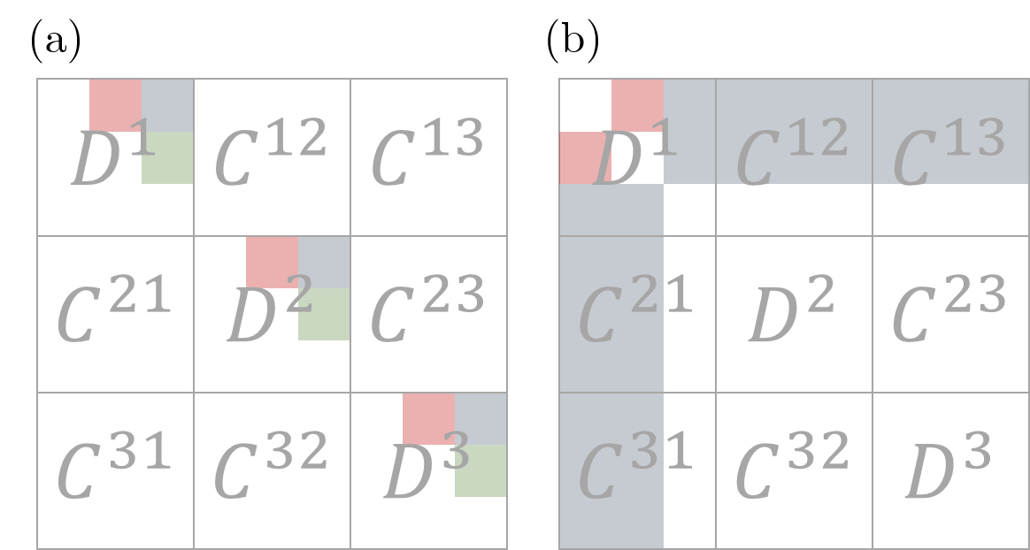
We will now present a particular (non-optimal) coherification procedure that can be applied to all quantum channels, irrespectively of their classical action . The coherence of channel coherified in such a way can thus be used as a lower-bound on the optimally coherified channel , i.e., and .
We start by reminding that the constraint not allowing one to completely coherify a channel is the TP condition, Eq. (8b), which means that . One can then choose all to be diagonal and try to coherify the channel only by modifying matrices. Note that the eigenvalues of are then given by the entries of , , where the vectors are defined by the rows of arranged in a non-increasing order,
| (32) |
From Theorem 2 we thus have that
| (33) |
The above majorization bound can be saturated by with the following choice of non-zero elements of . For each block find the maximal diagonal element, , and set the off-diagonal elements between them (elements of ) to the maximal value allowed by the CP condition, i.e., . Then, repeat the procedure for the -th largest eigenvalues of , , with . The structure of the resulting Jamiołkowski state is illustrated in Fig. 5 for . The spectrum of is given by
| (34) |
which is also the optimal spectrum for the Jamiołkowski state with a fixed diagonal, when we additionally assume no coherence in its diagonal blocks .
Let us now analyze the action of a channel coherified according to . We first note that a classical channel has the following Kraus decomposition:
| (35) |
so that the minimal number of Kraus operators is equal to the number of non-zero entries of a stochastic matrix (in general ). On the other hand, we know that, by construction, is equal to the sum over at most projectors, so that the number of the corresponding Kraus operators will be smaller or equal to . More precisely, one can obtain -th Kraus operator directly from the matrix: in every row of leave only the -th largest entry, replace it with its square root, and set all other entries to zero. For example, given the transition matrix from Eq. (31), we get
We thus see that it is always possible to coherify a channel , so that the number of Kraus operators (the rank of the Jamiołkowski state ) realizing a given classical transformation (with ) decreases from to . Physically, we can interpret as replacing classical processes (transitions from state to ) into a classical mixture over quantum processes, where each quantum process describes a coherent superposition of classical transitions, each to a different final state. We also note that there exist stochastic matrices for which one cannot reduce the number of Kraus operators below . These are given by transitions that move all populations to a fixed -th state, i.e., with all entries in the -th row equal to one and all other entries being zero. The matrices of the corresponding Jamiołkowski state are all vanishing, except for , which cannot be coherified due to the condition .
Finally, since it is always possible to coherify a channel so that the spectrum of its Jamiołkowski state is given by , one gets the following lower-bounds
| (36a) | |||||
| (36b) | |||||
For comparison with the upper-bounds presented in the previous section, Eqs. (30a) and (30b), we note that for the exemplary transition matrix used there, Eq. (31), we have
III.2.3 Qubits
Having described the general bounds on possible coherifications of quantum channels acting on arbitrary -dimensional spaces, we now want to focus on a particular case of . The classical action of a general qubit channel is given by a transition matrix described by two real parameters,
| (37) |
with . We will only focus on the case when , as the results for the case are analogous. Namely, one only needs to exchange with in all expressions, and transform all matrices by replacing with . The details of the derivations can be found in Appendix B.
For , Eq. (29) tells us that the spectrum of the Jamiołkowski state , corresponding to any channel with classical action specified by , is bounded in the following way,
| (38) |
This bound can be in fact saturated, i.e., there exists such that . Note that, since the majorization bound is saturated, both coherification procedures (maximising entropic and 2-norm coherence) coincide, and are simply denoted by . To express the Kraus operators of the corresponding optimally coherified channel , let us first introduce a unitary
| (39) |
and a decaying channel with
| (40) |
Then, with
| (41c) | ||||
| (41f) | ||||
It is straightforward to verify that the classical action of the resulting channel is given by [using Eq. (22)], as well as that the spectrum of the Jamiołkowski state is optimal [by checking that ]. Let us also explicitly emphasize that the optimally coherified channel is given by the composition of a unitary process and a decaying channel, . As a consequence there exists a pure state that is mapped by to a pure state , and therefore the minimum output entropy of is zero. We illustrate the action of on a Bloch sphere for a particular choice of in Fig. 6.
Finally, let us apply the notion of coherification to contribute to the studies on geometry of the set of one-qubit stochastic maps initiated in Ref. Ruskai et al. (2002).
Proposition 3.
Coherification of any classical one-qubit stochastic map, specified by a matrix from Eq. (37), yields a channel which is extremal in the set .
Proof.
In the bistochastic case , we obtain a unitary channel, which is extremal. In other cases, without loss of generality, we may assume that . The products of the Kraus operators from Eq. (40), corresponding to a decaying channel, read
| (42) |
Now, by direct inspection, we see that the above matrices form a linearly independent set. Thus, invoking the theorem of Choi Choi (1975), the channel described by two Kraus operators and is extremal. To see that is extremal, we note that the additional unitary matrix applied to Kraus operators will not introduce a linear dependence of the set defined in Eq. (42). ∎
III.2.4 Qutrits
We will now illustrate how our results can be applied beyond the simplest qubit scenario, by using them to find optimally coherified qutrit channels . Again, the coherification procedure will optimize both considered coherence measures simultaneously. The classical action of a general qutrit channel is given by a transition matrix described by six real parameters. Here, we will consider three families of such matrices, each parametrized by three real numbers:
| (43) |
with . We will refer to the above as cyclic matrices, single-row matrices and double-row matrices, respectively. For each family of we will provide the optimal spectrum of the Jamiołkowski state [which yields tight bounds on and via Eqs. (30a)-(30b)], as well as the Kraus decomposition of the optimally coherified channel . The details of the derivations can be found in Appendix C.
For cyclic matrices is given by , i.e., the optimal coherification procedure is given by the one we defined in Sec. III.2.2. Introducing
| (44) |
we thus get
| (45) |
The Kraus operators can be obtained by using the procedure described in Sec. III.2.2, e.g., for , and we get
| (46) |
For single-row transition matrices there are three separate cases depending on parameters , and . If then the optimal spectrum is given by
| (47) | |||||
and the Kraus decomposition of the corresponding optimally coherified channel is given by
| (48) |
If the number of non-zero elements of the optimal spectrum (so also of the Kraus operators) reduces from three to two. The optimal spectrum is again given by Eq. (45), but this time with
| (49) |
If we thus get , i.e., the optimal spectrum is constant for all parameters satisfying , and the Kraus operators of the optimal map are given by:
| (50) |
On the other hand, if then there is a slight change in the Kraus decomposition of the optimal map. Namely, the last rows of and in Eq. (50) are swapped.
For double-row matrices there are again three separate cases depending on the value of . These are specified by , and , and the optimal spectra are then given by
| (51a) | |||||
| (51b) | |||||
| (51c) | |||||
respectively. Due to the lack of concise expressions, we provide Kraus decompositions of the resulting optimally coherified channels in Appendix C.
III.2.5 Qudits
Finally, we want to make a short comment about a special family of channels in the general -dimensional case. Consider a completely contracting channel , which sends any initial state into a single point, . The corresponding Jamiołkowski state has a product structure and reads Życzkowski (2008). The output state can be coherified to a pure state by the standard procedure given in Eq. (5). Hence the contracting channel , can be coherified to a channel contracting into a pure state with and zero output entropy. Note that this coherification procedure increases the entropic coherence of a channel by . Notice also, that for a mixed state such a procedure is not optimal, as can be immediately seen by recalling the result presented in Sec. III.1, where we showed that can be completely coherified.
III.3 Bistochastic matrices and polygon constraints
We now proceed to the analysis of quantum channels whose classical action is described by bistochastic matrices that are not unistochastic (the middle shell of the graph presented in Fig. 4). On the one hand, due to Proposition 1, we know that these cannot be completely coherified. On the other, our majorization result derived in Sec. III.2.1 yields a trivial bound for bistochastic matrices. Moreover, a non-trivial constraint for all bistochastic matrices could serve as a witness of unistochasticity, and thus it is unlikely that such a concise bound can be found Bengtsson et al. (2005). Therefore, here we will present an approach that allows one to obtain limitations on possible coherifications of quantum channels with classical action described by a particular subset of .
We start by noting that due to the TP condition, Eq. (8b), for every we have (see Fig. 7a). This, via the polygon inequality, implies that
| (52) |
Recalling that matrices are all positive, we have
| (53) |
Combining the above two equations we arrive at
| (54) |
We thus see that the maximum value of allowed by CP condition is , whilst the TP condition restricts it via Eq. (54). Therefore, if for some we have
| (55) |
then is constrained beyond the positivity condition and we know that the resulting Jamiołkowski state cannot be pure, so that the corresponding channel cannot be completely coherified. More precisely, for every such that , we introduce
| (56) |
which describes the maximum fraction of the coherence (between states and of a matrix ) that could be achieved if there was no TP constraint.
Now, whenever (i.e., must be smaller than necessary for complete coherification), other off-diagonal elements of the Jamiołkowski state also become constrained beyond the positivity condition. Before we prove this and explain how it restricts the coherification of quantum channels, let us first comment on the condition. First of all, there exist that are neither unistochastic, nor they satisfy this condition for any . Thus, the presented bounds will, in general, work only for a subset of quantum channels with bistochastic classical action. However, as for a bistochastic matrix is either unistochastic or for some Bengtsson et al. (2005), we will obtain non-trivial bounds for all qutrit channels. Further improvements would require finding a clearer separation between the sets and .
We start by showing how can be used to constrain the purity of the optimally coherified channel. Note that Sylvester’s criterion states that implies that all submatrices of must have positive determinant. In particular, it means that for a part of a matrix containing , and any other we have
| (57) |
Since we know that the maximum value of is upper-bounded by , the above equation constrains all off-diagonal elements of sharing a row or column with or (see Fig. 7b). This results in the following bound on the purity of the optimally coherified Jamiołkowski state (see Appendix D for details):
| (58) |
with
| (59a) | |||||
| (59b) | |||||
and
| (60) |
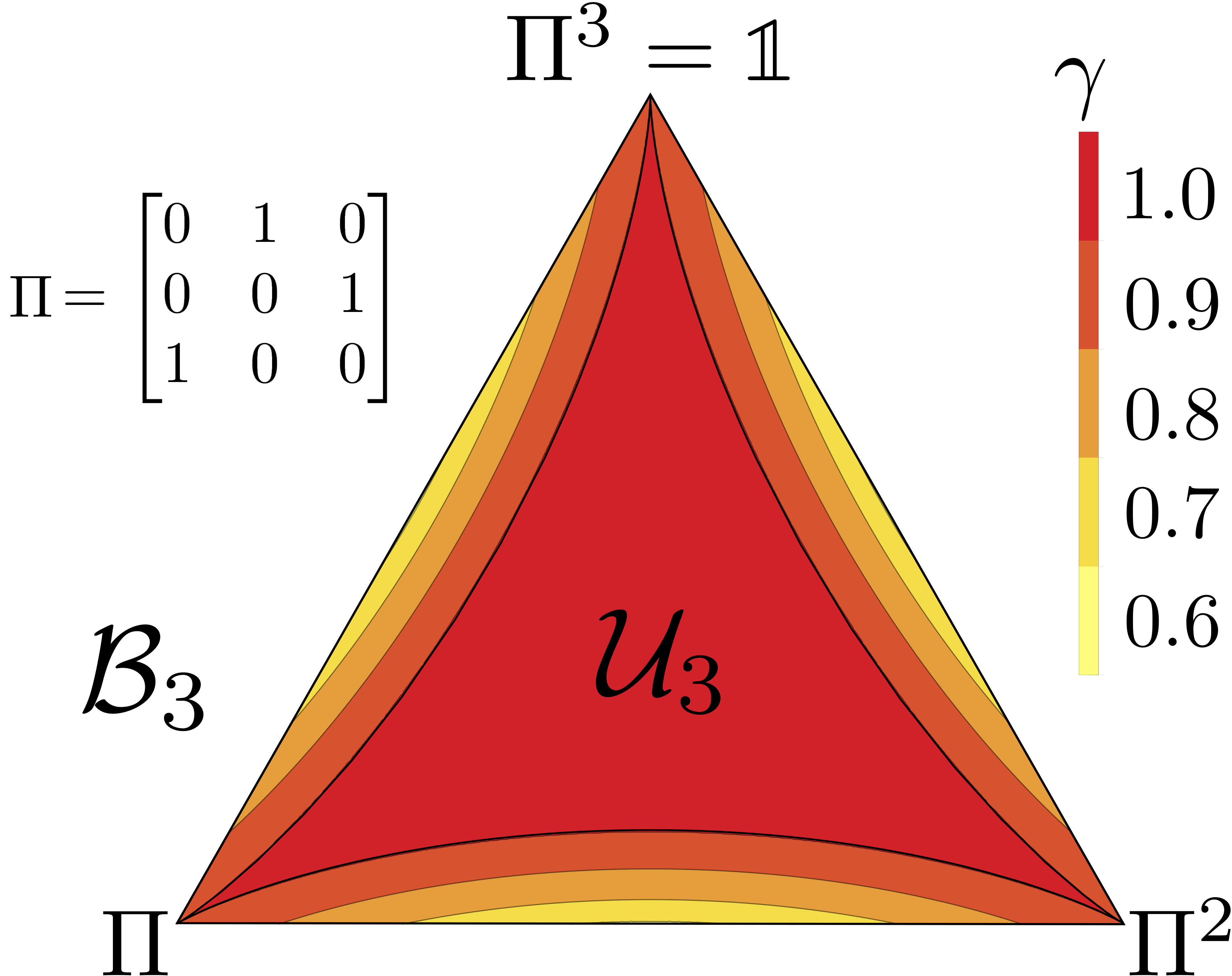
The purity deficits, and , add up for every for which Eq. (55) holds (however, care needs to be taken not to count twice the same terms). We illustrate this bound on the purity of the optimally coherified channel in Fig. 8 for an exemplary case of a family of qutrit maps.
Alternatively, one can use the fact that off-diagonal terms of are constrained beyond the positivity condition to bound , and then use Theorem 2 to obtain a non-trivial majorization bound on the eigenvalues of the Jamiołkowski state. In Appendix D we show for example that
| (61) |
with
| (62) |
where and are indices for which is minimized (so that we obtain non-trivial majorization bounds on the spectra of , whenever for some and ). This, in turn, means that
| (63) |
which can be used to obtain bounds on and via Eqs. (30a)-(30b). As an example consider a quantum channel with classical action given by
| (64) |
corresponding to the middle-point between and in Fig. 8. One then gets
| (65) |
resulting in , so that the spectrum of the optimally coherified Jamiołkowski state is majorized by .
Finally, let us note that, in particular cases, the tools introduced in Sec. III.2 can also be used to find limitations on coherifying channels with . As an example consider the family of qutrit channels described by cyclic matrices [first entry of Eq. (43)] with . The matrix is then bistochastic and the spectrum of the optimally coherified Jamiołkowski state is given by (for ) or (for ). This shows that the majorization bound, Eq. (63), applied to the channel with specified by Eq. (64) is tight.
IV Physical interpretation
We started this paper asking about the extent to which a given random transformation can be explained via the underlying deterministic and coherent process. Now, being equipped with formal bounds limiting possible coherifications of quantum channels, we will try to address this initial question. We will also provide interpretation of the purity of a channel by relating it to the notions of unitarity and average output purity. Finally, we will comment on the links and differences between our approach to the study of coherence of quantum channels, and the ones existing in the literature.
Let us start by recalling that the evolution of a pure quantum state under the action of a channel , described by
| (66) |
can be interpreted as an incoherent (probabilistic) mixture of different pure state transformations,
| (67) |
where
| (68) |
and we refer to the canonical Kraus form in which all Kraus operators are mutually orthogonal, as they are obtained by reshaping eigenvectors of the Choi-Jamiołkowski matrix. Each independent path, described by and being chosen with probability , describes a coherent evolution, as it preserves the ability of a state to interfere (it maps a pure state to a pure state). Thus, the probability distribution over different paths, , can be seen as describing the incoherent randomness associated with . Note, however, that the probability of evolving along a given path depends on the initial state of the system . In order to achieve a state-independent statement characterizing a given quantum channel , one can then focus on the average probability of choosing a given path. Introducing the average over (Haar distributed) pure states,
| (69) |
we see that the probability describing which path is chosen is on average333We note that the average here could actually be taken over all states, pure and mixed. However, in order to be consistent with the averaging process used in the definition of unitarity, we restrict the average to pure states only.
|
|
(70) |
where denotes, as usual, the eigenvalues of the Jamiołkowski state corresponding to .
We thus see that the incoherent randomness of the evolution coming from the random choice of different paths is (on average) described by the spectrum of . The extent to which a quantum channel with a given classical action can be coherified tells us how coherent the underlying evolution, leading to transitions described by , can be. On one extreme, we have unistochastic transitions that can be completely coherified and, therefore, explained by a single deterministic path (unitary dynamics). On the other hand, the majorization upper-bounds on that we derived in Sec. III, yield lower-bounds on the randomness of path distribution of the underlying process necessary to induce classical transformation . Moreover, our majorization lower-bound provides a particular coherent explanation of every classical process (decreasing the randomness of path distribution) and, in particular, shows that all transitions can be explained with at most paths.
Let us now focus on a particular measure describing the randomness of the path distribution, namely on the purity of a channel . One could be tempted to think that the bigger is, the purer the average output purity,
| (71) |
will be. Although the two notions are related, as we will shortly see, they are not in direct correspondence. As an illustrative example consider two quantum channels,
| (72a) | |||||
| (72b) | |||||
with classical action given by the van der Waerden matrix with flat entries , which maps every probability distribution to a uniform one. Both channels have the same average output purity equal to one; but for a reversible we have , while for an irreversible we get . This suggests that the purity of a channel is somehow related to reversibility of the process, which leads us to the concept of unitarity. It was originally introduced in Ref. Wallman et al. (2015) to measure the departure of a channel from the unitary dynamics, and for trace-preserving channels is defined by:
| (73) |
We note in the passing that one can also relate unitarity to the variance of the random variable :
| (74) |
For our exemplary channels we see that and , in accordance with the purity of the channel and capturing the fact that a completely irreversible process is as far as possible from a unitary transformation.
We will now formally relate , and . The authors of Ref. Wallman et al. (2015) showed that
| (75) |
which, using the definition of unitarity, directly leads to the general expression for the average output purity derived by Cappellini Cappellini (2007),
| (76) |
We thus see that both average output purity and unitarity are proportional to the purity of a channel corrected by a term describing the purity of the transformed maximally mixed state. Moreover, for large , actually approaches . Now, by noting that the minimal value of purity for a -dimensional system is , we obtain the following inequalities:444Note that by restricting to unital channels these inequalities actually become equalities.
| (77a) | ||||
| (77b) | ||||
Using our majorization and purity upper-bounds we can thus upper-bound the optimal unitarity of a channel with a given classical action . On the other hand, using the majorization lower-bound, we can lower-bound the average output purity of such an optimal channel. The above bounds can actually be tightened by noting that
| (78) |
Let us also mention that the optimally coherified qubit channel , with Kraus operators specified by Eqs. (41c) and (41f), not only maximizes purity, but also minimizes the output purity for the maximally mixed state [as it saturates the bound in Eq. (78)]. Therefore, it maximizes unitarity among all qubit channels with the same classical action.
Finally, we would like to relate the work presented here to studies on cohering power Mani and Karimipour (2015) and coherence generating power Zanardi et al. (2017a, b) of quantum channels. These notions were introduced within the framework of resource theory of coherence Baumgratz et al. (2014) and measure the ability of a channel to transform initially incoherent state to a coherent one. More formally they are defined by
| (79a) | |||||
| (79b) | |||||
where denotes the set of incoherent states ( if and only if for ), denotes the average over all incoherent states, and is any measure of coherence for states, e.g., the relative entropy of coherence . Since both definitions involve only the action of on incoherent states, we see that the only relevant parameters (defining the values of and ) are given by the diagonals of and , which are not constrained by the TP condition. Hence, given a fixed classical action of (so fixed diagonals of ), we can choose the diagonals of to be maximal possible (constrained only by complete positivity condition, ):
| (80) |
and set all other matrix elements of to zero. This way we will obtain a channel that maximizes both and among all channels with a fixed classical action . The action of such an optimal map is given by
| (81) |
with
| (82) |
We note that the above channels that maximize and for a fixed do not coincide with optimally coherified channels studied in this work. The reason for this is that the latter optimization depends on all coherence terms, whereas the former one only on the ones lying on the diagonal of . This emphasizes the main difference between our channel-oriented approach (when one focuses on the properties of the channel itself, specifically how close it is to a unitary evolution) and the state-oriented approach used in the studies of cohering power and coherence generating power (when one focuses on the properties of the output states for a restricted set of input states).
V Conclusions
Any classical state of size , represented by a diagonal density matrix , can be coherified to a pure state with maximal coherence, which is transformed back into by decoherence (see Fig. 2). In a similar way, one can try to coherify a quantum operation represented by the corresponding Jamiołkowski state . However, due to the trace preserving condition, the problem of coherifying a quantum channel has a much richer structure.
In this work we posed a general question: how to coherify a given classical map, represented by a stochastic transition matrix , in an optimal way? Physically, this can be understood as looking for the most coherent (deterministic) underlying quantum evolution that can explain the observed random transformation . Mathematically, among all quantum channels that decohere to we looked for the one whose Jamiołkowski state has maximal coherence (as measured by entropic and 2-norm coherence). We demonstrated that the complete coherification to a (reversible) unitary channel is possible if and only if is unistochastic, as schematically visualized in Fig. 3. To capture the limitations of possible coherifications of non-unistochastic maps we derived explicit bounds for the purity and entropy of the optimally coherified channel. Furthermore, we provided an explicit coherification procedure that allows one to lower-bound the coherence of the optimal channel, and solved the optimal coherification problem for several classes of channels, including all one-qubit channels.
Studying possible coherifications of quantum channels can also shed some light on the structure and geometry of the set of quantum operations Ruskai et al. (2002). For the set of pure quantum states (the Bloch sphere) can be obtained by coherifying the set of one-bit classical states. Analogously, the square of classical stochastic matrices forms a skeleton of the larger set of one-qubit quantum operations. Any unistochastic matrix can be coherified into a quantum unitary transformation, corresponding to a pure Jamiołkowski state . Furthermore, we have demonstrated that any classical transition matrix can be coherified to an optimal quantum channel, corresponding to a mixed state , that is an extremal point of . One would then like to check under what conditions a similar statement holds for higher dimensions, i.e., when the optimally coherified channels are extremal and have vanishing minimum output entropy.
Besides this problem concerning the geometry of , there are also other open questions that we would like to conclude this paper with. One could ask whether the optimally coherified channels are unique up to a unitary equivalence, i.e., can one find two channels whose Jamiołkowski states are not connected via unitary, and which maximize a given coherence measure among all Jamiołkowski states with a fixed diagonal? Furthermore, the expressions that lower- and upper-bound possible coherifications can definitely be improved, especially for bistochastic matrices. In this special case, exploring the boundary between unistochastic and bistochastic maps could be beneficial. Moreover, one might pursue a statistical approach and ask a question concerning a possible degree of coherification of a random stochastic matrix, or a generic quantum channel Bruzda et al. (2009). Last but not least, it would be very interesting to establish a closer connection between coherification approach to quantum channels, pursued in this work and based on the coherence of the corresponding Jamiołkowski states, with the earlier notion of the coherence power, related to the increase of coherence of selected quantum states by the action of a channel Mani and Karimipour (2015); García-Díaz et al. (2016); Zanardi et al. (2017b).
Note: Shortly after our work appeared on arXiv, another preprint studying the coherence of quantum channels was posted there Datta et al. (2017).
Acknowledgements
We would like to thank Valerio Cappellini for sharing with us his unpublished notes and Antony Milne for his invaluable linguistic advices. We acknowledge financial support from the ARC via the Centre of Excellence in Engineered Quantum Systems, project number CE110001013 (K.K.) and Polish National Science Centre under the project numbers 2016/22/E/ST6/00062 (Z.P.) and DEC-2015/18/A/ST2/00274 (K.Ż.).
Appendix A Proof of Theorem 2
We will make use of the following known results (see Lemma 3.4 of Ref. Bourin and Lee (2012) and Eq. (2.5) of Ref. Ando (1994)):
Lemma 4.
For every positive semi-definite matrix written in blocks we have the following decomposition
| (83) |
for some unitary operators and .
Lemma 5.
For denoting the vector of eigenvalues of arranged in a decreasing order we have
| (84) |
We are now ready to present the proof of Theorem 2.
Appendix B Coherifying qubit channels
Before we proceed to deriving the results presented in the main text, let us first recall the following fact. Given two channels, and , whose Jamiołkowski states, and , are connected via a local unitary acting on the second subsystem, , their Kraus decomposition satisfies
| (86) |
Now, using the block structure of the Jamiołkowski state, Eq. (12), and taking into account the TP condition, , for a general qubit channel, we get:
| (87) |
Consider a unitary diagonalizing , i.e., . Now, the same unitary will obviously also diagonalize . Therefore, a unitary diagonalizes the blocks of the Jamiołkowski state :
| (88) |
where blank spaces mean arbitrary entries, and .
For we may obtain the optimally coherified state [with the spectrum saturating the bound given by from Eq. (38)] in the following way. We choose (resulting in ), and set the off-diagonal element between and to the maximal value allowed by positivity, i.e., . As a result, becomes a projector on two orthogonal pure states, which in turn means that the corresponding map is given by the decaying Kraus operators from Eq. (40). Since , we can use Eq. (86), to find the Kraus of decomposition of given by . Finally, is defined by , which is exactly the unitary given in Eq. (39) (note that, since is real, we have )
Similarly, for we may choose (resulting in ), and set the off-diagonal element between and to the maximal value allowed by positivity, i.e., . As described in the main text, this then leads to the same results as in case, just with and exchanged, as well as with all matrices transformed by replacing with .
Appendix C Coherifyng qutrit channels
C.1 Cyclic matrices
The general form of matrices is as follows:
|
|
Clearly, in order to satisfy the TP condition, , we need . Hence, the Jamiołkowski state can be recast in the following form (note that columns and rows number 1, 5 and 9, composed only of zeros, have been removed):
| (89) |
Now, using Theorem 2, we get:
| (90) |
where
| (91) |
Moreover, one can construct optimally coherified matrix such that . To do this one simply needs to group together the maximal/minimal terms of each matrix and set the corresponding off-diagonal terms to the maximal values allowed by the positivity constraint. For example, if , and , one chooses
and sets the rest of off-diagonal terms to zero. Note that this is exactly the construction introduced in Sec. III.2.2 and illustrated in Fig. 5.
C.2 Single-row matrices
The general form of matrices is as follows:
|
|
Clearly, in order to satisfy the TP condition we need and . We now note that a unitary matrix diagonalizing ,
| (92) |
also diagonalizes (by keeping it unchanged) and . Therefore, a unitary diagonalizes the blocks of the Jamiołkowski state :
| (93) |
where blank spaces mean arbitrary entries and .
Without loss of generality let us assume that . Then, using Theorem 2, we get with given by
|
|
where denotes the second largest element of the set. Note also that, for fixed , the vector is just a function of , since . Now, maximising maximizes both and (recall that is constant and equal to 1), and so for . In order to find the optimal (optimal meaning that for all we have ) we thus need to maximize . Recalling that we have two constraints, and , we arrive at two cases.
For the maximal (and thus optimal) value of is , which also results in . The optimal bounding vector is then given by
|
|
(94) |
Moreover, one can construct the Jamiołkowski state that saturates this optimal bound, i.e., . This can be achieved, again, by setting the adequate off-diagonal terms in Eq. (93) to the maximal possible value allowed by the positivity condition. More precisely, we group , and together, leaving the remaining two terms, and , ungrouped. As a result, becomes a projector on three orthogonal pure states, which in turn means that the corresponding map is given by the following Kraus operators:
Finally, using Eq. (86) we conclude that the Kraus operators corresponding to the optimally coherified channel (with Jamiołkowski state ) are given by with as above and defined by Eq. (92) with and , i.e.,
| (95) |
For the maximal (and thus optimal) value of is , which also results in . The optimal bounding vector is then given by
|
|
(96) |
The bound can be saturated in a usual way – by proper grouping of diagonal elements and setting the corresponding off-diagonal elements to the maximal value allowed by the positivity condition. If then we group together , and , with and forming the other group; otherwise we group together , and , with and forming the other group. In the former case the resulting Kraus operators of the optimally coherified channel read
and in the latter case they read
with in both cases defined by Eq. (92) with and , i.e.,
| (97) |
C.3 Double-row matrices
The general form of matrices is as follows:
|
|
We now note that a unitary matrix diagonalizing ,
|
|
(98) |
also diagonalizes and (by keeping it unchanged). Therefore, a unitary diagonalizes the blocks of the Jamiołkowski state :
| (99) |
where blank spaces mean arbitrary entries and . To shorten the notation we define .
Without loss of generality we may assume , so that . Then, using Theorem 2, we have
|
|
(100) |
Now, we observe that for and . We thus aim at maximising the largest eigenvalue of while minimizing its smallest eigenvalue. Again, noting that we are constrained by and we arrive at three distinct cases dependent on the value of .
For the maximal (and thus optimal) value of is , which also results in . The optimal bounding vector is then given by
| (101) |
The above optimal spectrum can be realized by the Jamiołkowski state by simply setting in Eq. (99) the off-diagonal terms between and (or ) to . Recalling the relation between the Kraus operators corresponding to Jamiołkowski states connected via a local unitary, Eq. (86), we find that the Kraus decomposition of the optimally coherified channel is given by:
with being a unitary such that
| (102) |
and denoting arbitrary entries as long as stays unitary, e.g.,
Also note that the position of in matrices describing and can be exchanged.
For the optimal values are and . The optimal bounding vector is then given by
| (103) |
which can be achieved by the coherified Jamiołkowski state in an analogous way to the first case. This leads to the following decomposition of into the set of Kraus operators,
with being a unitary such that
| (104) |
and denoting arbitrary entries as long as stays unitary, e.g.,
| (105) |
Again, we note that the position of in matrices describing and can be exchanged.
Finally, for the optimal values are , and . The optimal bounding vector is then given by
| (106) |
The above spectrum can be achieved by the optimally coherified Jamiołkowski state by setting the off-diagonal terms in Eq. (99) appropriately. More precisely, one chooses the term between and to be , and the term between and to be . The resulting Kraus operators are given by
| (107) |
with
| (108) |
if and
| (109) |
if .
Appendix D Polygon constraints
First, we derive the expression for the purity bound, Eq. (58). The expression for , Eq. (59a), comes directly from the fact that . To obtain , Eq. (59b), let us start by parametrizing the matrix from Eq. (57), i.e., the submatrix of , in the following way
| (110) |
with . We then have if and only if
| (111) |
Now, our aim is to upper-bound the squared moduli of the off-diagonal terms of (for fixed ), given the above constraint and the fact that for some . First, assume that is fixed, so that effectively we want to find the maximum of (in fact, the optimal choice is to maximize , i.e., set ). It is straightforward to check that it is achieved at the boundary of the constraint, i.e., when Eq. (111) becomes an equality. One can then solve for , substitute it to , and find the maximum of the resulting expression over . This leads to the following bound on the off-diagonal terms of :
| (112) |
with defined in Eq. (60). As in order to achieve unit purity one needs , the above bound leads to the following deficit of purity:
| (113) |
Finally, the above deficit adds up for every choice of not equal to or (i.e., for all off-diagonal elements sharing row or column with or in Fig. 7b), so that using , we finally arrive at Eq. (59b).
We now proceed to the proof of the majorization bound, Eq. (61). Note that, using Lemma 4 from Appendix A, we can rewrite (up to permutations) as
| (114) |
with
| (115) |
and being unitary. The eigenvalues of are given by
| (116) |
whereas the largest eigenvalue of is constrained by
|
|
(117) |
where we used the fact that is bistochastic. Thus, using Lemma 5 and choosing and minimizing , we arrive at Eq. (61).
Note that the above construction can be easily generalized to cases where for a given there are many pairs for which . Instead of a matrix , one simply chooses it to contain all off-diagonal elements of that are constrained beyond the positivity condition, finds its eigenvalues, and obtains a tighter bound using Lemma 5 again.
References
- Zhang et al. (1990) W.-M. Zhang, D. H. Feng, and R. Gilmore, “Coherent states: Theory and some applications,” Rev. Mod. Phys. 62, 867 (1990).
- Baumgratz et al. (2014) T. Baumgratz, M. Cramer, and M. B. Plenio, “Quantifying coherence,” Phys. Rev. Lett. 113, 140401 (2014).
- Brandão and Gour (2015) F. G. S. L. Brandão and G. Gour, “The general structure of quantum resource theories,” Phys. Rev. Lett. 115, 070503 (2015).
- Streltsov et al. (2016) A. Streltsov, G. Adesso, and M. B. Plenio, “Quantum coherence as a resource,” arXiv:1609.02439 (2016).
- Mani and Karimipour (2015) A. Mani and V. Karimipour, “Cohering and decohering power of quantum channels,” Phys. Rev. A 92, 032331 (2015).
- García-Díaz et al. (2016) M. García-Díaz, D. Egloff, and M. B. Plenio, “A note on coherence power of -dimensional unitary operators,” Quant. Inf. Comp. 16, 1282 (2016).
- Zanardi et al. (2017a) P. Zanardi, G. Styliaris, and L. C. Venuti, “Coherence-generating power of quantum unitary maps and beyond,” Phys. Rev. A 95, 052306 (2017a).
- Zanardi et al. (2017b) P. Zanardi, G. Styliaris, and L. C. Venuti, “Measures of coherence-generating power for quantum unital operations,” Phys. Rev. A 95, 052307 (2017b).
- (9) Z. Xi, M. Hu, Y. Li, and H. Fan, “Entropic characterization of coherence in quantum evolutions,” arXiv:1510.06473 .
- Bu et al. (2017) K. Bu, A. Kumar, L. Zhang, and J. Wu, “Cohering power of quantum operations,” Phys. Lett. A 381, 1670–1676 (2017).
- Jamiołkowski (1972) A. Jamiołkowski, “Linear transformations which preserve trace and positive semidefiniteness of operators,” Rep. Math. Phys. 3, 275–278 (1972).
- Choi (1975) M.-D. Choi, “Completely positive linear maps on complex matrices,” Linear Algebra Appl. 10, 285–290 (1975).
- Życzkowski and Bengtsson (2004) K. Życzkowski and I. Bengtsson, “On duality between quantum maps and quantum states,” Open Syst. Inf. Dyn. 11, 3–42 (2004).
- Wallman et al. (2015) J. Wallman, C. Granade, R. Harper, and S. T. Flammia, “Estimating the coherence of noise,” New J. Phys. 17, 113020 (2015).
- Nielsen and Chuang (2010) M. A. Nielsen and I. L. Chuang, Quantum computation and quantum information (Cambridge University Press, 2010).
- Bengtsson and Życzkowski (2017) I. Bengtsson and K. Życzkowski, Geometry of Quantum States, II ed. (Cambridge University Press, 2017).
- Lostaglio et al. (2015a) M. Lostaglio, D. Jennings, and T. Rudolph, “Description of quantum coherence in thermodynamic processes requires constraints beyond free energy,” Nat. Commun. 6, 6383 (2015a).
- Lostaglio et al. (2015b) M. Lostaglio, K. Korzekwa, D. Jennings, and T. Rudolph, “Quantum coherence, time-translation symmetry, and thermodynamics,” Phys. Rev. X 5, 021001 (2015b).
- Åberg (2006) J. Åberg, “Quantifying superposition,” arXiv:0612146 (2006).
- Lakshminarayan et al. (2014) A. Lakshminarayan, Z. Puchała, and K. Życzkowski, “Diagonal unitary entangling gates and contradiagonal quantum states,” Phys. Rev. A 90, 032303 (2014).
- Tadej and Życzkowski (2006) W. Tadej and K. Życzkowski, “A concise guide to complex Hadamard matrices,” Open Syst. Inf. Dyn. 13, 133–177 (2006).
- Kleinmann et al. (2006) M. Kleinmann, H. Kampermann, T. Meyer, and D. Bruß, “Physical purification of quantum states,” Phys. Rev. A 73, 062309 (2006).
- Roga et al. (2011) W. Roga, M. Fannes, and K. Życzkowski, “Entropic characterization of quantum operations,” Int. J. Quantum Inf. 9, 1031–1045 (2011).
- Dunkl and Życzkowski (2009) C. Dunkl and K. Życzkowski, “Volume of the set of unistochastic matrices of order 3 and the mean Jarlskog invariant,” J. Math. Phys. 50, 123521 (2009).
- Bengtsson et al. (2005) I. Bengtsson, Å. Ericsson, M. Kuś, W. Tadej, and K. Życzkowski, “Birkhoff’s polytope and unistochastic matrices, and ,” Commun. Math. Phys. 259, 307–324 (2005).
- Li and Woerdeman (1997) C.-K. Li and H. J. Woerdeman, “Special classes of positive and completely positive maps,” Linear Algebra Appl. 255, 247–258 (1997).
- Levick et al. (2017) J. Levick, D. W. Kribs, and R. Pereira, “Quantum privacy and Schur product channels,” arXiv:1709.01752 (2017).
- Ruskai et al. (2002) M. B. Ruskai, S. Szarek, and E. Werner, “An analysis of completely-positive trace-preserving maps on ,” Linear Algebra Appl. 347, 159–187 (2002).
- Życzkowski (2008) K. Życzkowski, “Quartic quantum theory: an extension of the standard quantum mechanics,” J. Phys. A 41, 355302 (2008).
- Cappellini (2007) V. Cappellini, private communication (2007).
- Bruzda et al. (2009) W. Bruzda, V. Cappellini, H.-J. Sommers, and K. Życzkowski, “Random quantum operations,” Phys. Lett. A 373, 320 (2009).
- Datta et al. (2017) C. Datta, S. Sazim, A. K. Pati, and P. Agrawal, “Coherence of quantum channels,” arXiv:1710.05015 (2017).
- Bourin and Lee (2012) J.-C. Bourin and E.-Y. Lee, “Unitary orbits of Hermitian operators with convex or concave functions,” Bull. London Math. Soc. 44, 1085–1102 (2012).
- Ando (1994) T. Ando, “Majorizations and inequalities in matrix theory,” Linear Algebra Appl. 199, 17–67 (1994).