All tree level scattering amplitudes in Chern-Simons theories with fundamental matter

Abstract

We show that Britto-Cachazo-Feng-Witten (BCFW) recursion relations can be used to compute all tree level scattering amplitudes in terms of $2\rightarrow 2$ scattering amplitude in $U(N)$ ${\mathcal{N}}=2$ Chern-Simons (CS) theory coupled to matter in fundamental representation. As a byproduct, we also obtain a recursion relation for the CS theory coupled to regular fermions, even though in this case standard BCFW deformations do not have a good asymptotic behaviour. Moreover at large $N$, $2\rightarrow 2$ scattering can be computed exactly to all orders in ’t Hooft coupling as was done in earlier works by some of the authors. In particular, for ${\mathcal{N}}=2$ theory, it was shown that $2\rightarrow 2$ scattering is tree level exact to all orders except in the anyonic channel Inbasekar et al. (2015), where it gets renormalized by a simple function of ’t Hooft coupling. This suggests that it may be possible to compute the all loop exact result for arbitrary higher point scattering amplitudes at large $N$.

I Introduction

Chern-Simons (CS) gauge theories coupled to matter fields have a wide variety of applications in areas as diverse as quantum hall physics, anyonic physics, topology of three manifolds, quantum gravity via the AdS/CFT correspondence, etc. In particular, CS theories coupled to matter in fundamental representation Aharony et al. (2012a); Giombi et al. (2012) are conjectured to enjoy a strong weak duality, which follows from the study of their corresponding bulk duals Klebanov and Polyakov (2002); Sezgin and Sundell (2002); Giombi and Yin (2010); Giombi et al. (2012). Moreover, at large N, these theories are exactly solvable Aharony et al. (2012a); Giombi et al. (2012); Maldacena and Zhiboedov (2013a, b). This led to impressive large $N,\kappa$ (keeping the ’t Hooft coupling $\lambda=\frac{N}{\kappa}$ fixed) computations to all orders in the ’t Hooft coupling in both sides of duality and hence verifying the duality quite convincingly. These computations include exact multipoint current correlators Aharony et al. (2012b); Gur-Ari and Yacoby (2013); Gurucharan and Prakash (2014); Bedhotiya and Prakash (2015); GurAri and Yacoby (2015); Geracie et al. (2016); Gur-Ari et al. (2016), exact partition function Giombi et al. (2012); Jain et al. (2012); Yokoyama (2013); Aharony et al. (2013); Jain et al. (2013a); Takimi (2013); Jain et al. (2013b); Yokoyama (2014); Minwalla and Yokoyama (2016); Nosaka and Yokoyama (2018), and exact S-matrices Jain et al. (2015); Dandekar et al. (2015); Inbasekar et al. (2015); Yokoyama (2016). See also GurAri and Yacoby (2015); Giombi et al. (2017); Wadia (2016); Radicevic et al. (2016); Giombi (2017) for further checks of duality. Recently, the duality was made more precise in Radicevic (2016); Aharony (2016); Seiberg et al. (2016); Karch and Tong (2016) and subsequently generalized to finite N in Karch et al. (2017); Hsin and Seiberg (2016); Aharony et al. (2017); Benini et al. (2017); Gaiotto et al. (2017); Jensen and Karch (2017a, b). An example of the strong-weak duality is the duality between CS gauge theory coupled to fundamental fermions and CS gauge theory coupled to fundamental critical bosons. Other examples include self dual theories, such as ${\mathcal{N}}=1$, ${\mathcal{N}}=2$ supersymmetric CS matter theories. At large $N$, it was demonstrated that the S matrix for the $2\to 2$ scattering computed exactly to all orders in the ’t Hooft coupling displays an unusual modified crossing relation Jain et al. (2015); Inbasekar et al. (2015); Yokoyama (2016). Moreover, for ${\mathcal{N}}=2$ theory, the result is tree level exact Inbasekar et al. (2015) except in the anyonic channel, where it gets renormalized by a simple function of the ’t Hooft coupling.

A natural question to ask would be, is it possible to compute arbitrary $m\rightarrow n$ scattering amplitudes at all values of the ’t Hooft coupling at large $N,\kappa$? Given the simplicity of the results at least in the supersymmetric case, it is also interesting to ask if the computability of scattering amplitudes extends to finite $N,\kappa$. As a first step towards these questions, we compute all tree level amplitudes for the ${\mathcal{N}}=2$ theory and the regular fermionic theory. We show that a $m\rightarrow n$ scattering amplitude can be computed recursively in terms of the $2\to 2$ scattering amplitudes in these theories. Similar recursion relations in three dimensions were first developed in Gang et al. (2011), in the context of the Aharony-Bergman-Jafferis-Maldacena (ABJM) theory and subsequently applied to other theories like 3d super-Yang-Mills in Lipstein and Mason (2013) and massive 3d $\mathcal{N}=2$ gauge theories in Agarwal et al. (2014). Note that, the self-dual $\mathcal{N}=2$ supersymmetric theory is particularly interesting and important since via RG flow, we can obtain non supersymmetric dual pairs such as critical bosons coupled to CS and regular fermions coupled to Chern-Simons Jain et al. (2013b); GurAri and Yacoby (2015).

II Four point scattering amplitude

In this Letter, we compute scattering amplitudes in fermion coupled to $SU(N)$ CS theory (FCS)

$$\int d^{3}x\biggl{[}-\frac{\kappa}{4\pi}\epsilon^{\mu\nu\rho}\text{Tr}\left(A_{\mu}\partial_{\mu}A_{\rho}-\frac{2i}{3}A_{\mu}A_{\nu}A_{\rho}\right)+\bar{\psi}i\not{\mathcal{D}}\psi\biggr{]}\ ,$$ (1)

and in ${\mathcal{N}=2}$ CS matter theory coupled to a Chiral multiplet given by

$$\mathcal{S}_{\mathcal{N}=2}^{L}=\int d^{3}x\biggl{[}-\frac{\kappa}{4\pi}\epsilon^{\mu\nu\rho}\text{Tr}\left(A_{\mu}\partial_{\mu}A_{\rho}-\frac{2i}{3}A_{\mu}A_{\nu}A_{\rho}\right)$$

$$\quad+\bar{\psi}i\not{\mathcal{D}}\psi-\mathcal{D}^{\mu}\bar{\phi}\mathcal{D}_{\mu}\phi+\frac{4\pi^{2}}{\kappa^{2}}(\bar{\phi}\phi)^{3}+\frac{4\pi}{\kappa}(\bar{\phi}\phi)(\bar{\psi}\psi)$$

$$+\frac{2\pi}{\kappa}(\bar{\psi}\phi)(\bar{\phi}\psi)\biggr{]}\ .$$ (2)

For our purposes, it is convenient to introduce the spinor helicity basis Elvang and Huang (2015) defined by

$$p_{i}^{\alpha\beta}=p_{i}^{\mu}\sigma_{\mu}^{\alpha\beta}=\lambda_{i}^{\alpha}\lambda_{i}^{\beta},~{}~{}(p_{i}+p_{j})^{2}=2p_{i}.p_{j}=\langle\lambda_{i}^{\alpha}\lambda_{i,\alpha}\rangle^{2}\ .$$ (3)

Below we use the notation $\langle\lambda_{i}^{\alpha}\lambda_{j,\alpha}\rangle=\langle ij\rangle.$ For a supersymmetric amplitude, the standard procedure involves introduction of on-shell grassman variables $\theta$ such that the super-creation and super-annihilation operators are given by

$$A_{i}=a_{i}+\theta_{i}\alpha_{i},~{}~{}A_{i}^{\dagger}=\theta_{i}a^{\dagger}_{i}+\alpha^{\dagger}_{i},$$ (4)

where $\left(a^{\dagger}_{i},a_{i}\right)$/$\left(\alpha^{\dagger}_{i},\alpha_{i}\right)$ create and annihilate a boson/fermion with momenta $p_{i}$ respectively. The two on-shell supercharges for $n$ point scattering amplitudes are given by

$$Q=\sum_{i=1}^{n}q_{i}=\sum_{i=1}^{n}\lambda_{i}\theta_{i},~{}~{}{\bar{Q}}=\sum_{i=1}^{n}{\bar{q}}_{i}=\sum_{i=1}^{n}\lambda_{i}\partial_{\theta_{i}}\ .$$ (5)

For FCS theory in (1), the tree level $2\to 2$ scattering amplitude is given by Jain et al. (2015)

$$A_{4}^{F}=\langle\bar{\psi}(p_{1})\psi(p_{2})\bar{\psi}(p_{3})\psi(p_{4})\rangle=\frac{\langle 12\rangle\langle 24\rangle}{\langle 23\rangle}\delta(\sum_{i=1}^{4}p_{i})\ .$$ (6)

For ${\mathcal{N}=2}$ theory in (II), the tree level $2\to 2$ super amplitude is given by

$$A_{4}^{S}=\frac{\langle 12\rangle}{\langle 23\rangle}\delta(\sum_{i=1}^{4}p_{i})Q^{2}=\frac{\langle 12\rangle}{\langle 23\rangle}\delta(\sum_{i=1}^{4}p_{i})\sum_{1=i<j}^{4}\langle ij\rangle\theta_{i}\theta_{j}\ .$$ (7)

Here $A_{4}^{S}$ is the super-amplitude computed using the super-creation/annihilation operators defined in (4). Any component amplitude can be obtained from (7) by picking up the coefficient of products of two $\theta$’s.

III Higher point scattering amplitude

BCFW recursion relations are an efficient method to compute and express arbitrary higher point scattering amplitudes in terms of product of lower point amplitudes. Standard procedure for BCFW involves the deformation of two external momenta of the particles by a complex parameter $z$ such that the particles continue to remain “on shell” and the total momentum conservation of the process continues to hold. In $3D$, BCFW deformations are a little different than in $4D$ and were first discussed in Gang et al. (2011) (We follow their notations closely). BCFW recursion relations are applicable in $3D$ provided that the higher point amplitudes are regular functions at both $z\to\infty$ and $z\to 0$. In the following section we study the $z\to\infty$ (and $z\rightarrow 0$) behavior of the amplitudes in the theories described earlier. We find it convenient to deform color contracted (we label them as ‘$1$’and ‘$2$’) external legs. In 3-dimensions, momentum deformation of particles 1 and 2 can be written in terms of the spinor-helicity variables as

$$\left(\begin{array}[]{c}{\hat{\lambda}}_{1}\\ {\hat{\lambda}}_{2}\end{array}\right)=R\left(\begin{array}[]{c}\lambda_{1}\\ \lambda_{2}\end{array}\right),~{}~{}\rm{where}~{}~{}~{}R=\left(\begin{array}[]{cc}\frac{z+z^{-1}}{2}&-\frac{z-z^{-1}}{2~{}i}\\ \frac{z-z^{-1}}{2~{}i}&\frac{z+z^{-1}}{2}\end{array}\right)\ .$$ (8)

In the theories (1),(II), all 3-point vertices involve gauge fields and since the CS gauge field does not have an on shell propagating degree of freedom, it follows that only even-point functions are non-zero. This also implies that the 4-point functions are fundamental building blocks for higher point functions.

Under the deformation (8), any tree-level scattering amplitude for FCS in (1) is not well behaved at large $z$ and hence doesn’t obey the requirements of BCFW. However this situation is cured for the ${\mathcal{N}=2}$ theory defined in (II). Additionally, conservation of the super-charges in (5) require that the on-shell spinor variables $\theta$ be deformed as

$$\left(\begin{array}[]{c}{\hat{\theta}}_{1}\\ {\hat{\theta}}_{2}\end{array}\right)=R\left(\begin{array}[]{c}\theta_{1}\\ \theta_{2}\end{array}\right)\ ,$$ (9)

where the $R$ matrix is defined by (8).

Let us denote the $2n-$point super-amplitude as $A_{2n}(\lambda_{1},\lambda_{2},\cdots\lambda_{2n},\theta_{1},\theta_{2},\cdots\theta_{2n})$ and the deformed amplitude by $A_{2n}({\hat{\lambda}}_{1},{\hat{\lambda}}_{2},\cdots\lambda_{2n},{\hat{\theta}}_{1},{\hat{\theta}}_{2},\cdots\theta_{2n},z)$. The deformed super-amplitude can be explicitly written as an expansion in the $\theta$ variables as follows

$$A_{2n}(z) =A^{0}(z)+A^{1}(z){\hat{\theta}}_{1}(z)+A^{2}(z){\hat{\theta}}_{2}(z)$$

$$\hskip 85.35826pt+A^{12}(z){\hat{\theta}}_{1}(z){\hat{\theta}}_{2}(z)$$

$$=A^{0}(z)+{\tilde{A}}^{1}(z)\theta_{1}+{\tilde{A}}^{2}(z)\theta_{2}+A^{12}(z)\theta_{1}\theta_{2},$$ (10)

where in the last line of (III) we have used (8) and the fact that ${\hat{\theta}}_{1}(z){\hat{\theta}}_{2}(z)=\theta_{1}\theta_{2}$. We have also defined

$$\begin{pmatrix}\tilde{A}^{1}(z)\\ \tilde{A}^{2}(z)\end{pmatrix}=R^{T}\begin{pmatrix}A^{1}(z)\\ A^{2}(z)\end{pmatrix}\ ,$$ (11)

where $R^{T}$ is the transpose of the R matrix defined in (8), with $RR^{T}=1$. The super-momentum conservation implies that the large $z$ behavior of the super-amplitude $A_{2n}(z)$ is identical to that of the components $A^{0},A^{12}$. Hence it is sufficient to show that either of $A^{0}$ or $A^{12}$ are well behaved since supersymmetric ward identity guarantees the required behavior for the rest of the amplitudes. It is convenient to write the fields in pair wise contractions since they transform in the fundamental representation of the gauge group. For instance we are interested in the large z behavior of amplitudes such as $(\bar{\psi}_{1}^{i}\phi_{2i})(\bar{\phi}_{3}^{j}\psi_{4j})\ldots$ and $(\bar{\phi}_{1}^{i}\psi_{2i})(\bar{\psi}_{3}^{j}\phi_{4j})\ldots$, where $\ldots$ represent color contracted bosonic or fermionic particles allowed by interactions in (II). These amplitudes appear in $A^{0},A^{12}$ in (III) respectively.

We have checked explicitly by Feynman diagrams that the amplitude $A^{0}=A_{6}(\bar{\psi}_{1}\phi_{2}\bar{\phi}_{3}\psi_{4}\bar{\phi}_{5}\phi_{6})$ is well behaved. We discuss the large $z$ behavior of the general $2n$ point amplitude using the background field method Arkani-Hamed and Kaplan (2008) in the next section.

IV Asymptotic behavior of amplitudes

To understand the large $z$ behavior of various scattering amplitudes, it is extremely useful to think from the background field method point of view introduced in Arkani-Hamed and Kaplan (2008). Here $z$-deformed particles are considered as hard particles propagating in a background of soft particles. The amplitude is modified due to (a) modified propagator of intermediate hard particle; (b) the modified contribution of various vertices; and, (c) modified fermion wave function, in case an external deformed particle is a fermion. Detailed analysis shows (we follow closely Arkani-Hamed and Kaplan (2008); Gang et al. (2011)) that the non-trivial $z\to\infty$ behavior of the amplitude is due to diagrams of the kind depicted in fig. 1.

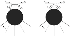
Figure 1: The diagrams that have a non-regular $z\to\infty$ behavior. $\mathcal{O}(z)$ part of these two diagrams cancel against each other to give a regular $z\to\infty$ behavior of the total amplitude. In the above diagram, the solid lines correspond to fermions and the dashed lines correspond to bosons. This amplitude appears in $A^{0}$ in (III). The gray coloured lines corresponds to deformed hard particle.

The values of these diagrams are:

$$\!\!\!\text{Gauge-field exchange: }\frac{4\pi i}{\kappa}\langle k_{4}|\gamma^{\mu}|1\rangle\frac{k_{3}^{\nu}p_{2}^{\rho}}{(k_{3}+p_{2})^{2}}\epsilon_{\mu\nu\rho}$$ (12)

$$\text{Contact vertex: }-\frac{2\pi}{\kappa}\langle k_{4}|1\rangle$$ (13)

Under the 1-2 $z$-deformations, (8), in the $z\to\infty$ limit the $\mathcal{O}(z)$ part of the amplitude cancels and the amplitude behaves as $\mathcal{O}(1/z)$. Hence this amplitude has a regular $z\to\infty$ behavior for ${\mathcal{N}}=2$ theory. This cancellation works even for the 4-point function $\langle\bar{\psi}_{1}\phi_{2}\bar{\phi}_{3}\psi_{4}\rangle$, which receives contributions from the diagrams in fig. 1 with the blob removed and $k_{3}\to p_{3},k_{4}\to p_{4}$ are taken to be on-shell momenta. It is important to emphasize that we need minimum ${\mathcal{N}}=2$ amount of supersymmetry for this to work .

V Recursion relations in $\mathcal{N}=2$ theory

Figure 2: Recursion formula for a 2n point amplitude: The black lines denote the undeformed legs, the external gray lines represent the deformed legs and $p_{f}$ represents the momentum in the factorization channel.

In the last section, we have demonstrated that $A^{0}$ is well behaved in large $z$. Hence we can apply the BCFW recursion relation directly to the super amplitude in the left hand side of (III). The recursion formula for a $2n$ point superamplitude can be expressed in terms of lower point superamplitudes as follows (see fig 2)

$$A_{2n}(z=1)=\sum_{f}\int\frac{d\theta}{p_{f}^{2}}\biggl{(}z_{a;f}\frac{z_{b;f}^{2}-1}{z_{a;f}^{2}-z_{b;f}^{2}}A_{L}(z_{a;f},\theta)A_{R}(z_{a;f},i\theta)+(z_{a;f}\leftrightarrow z_{b;f})\biggr{)},$$ (14)

$$\left(z_{a;f}^{2}~{},~{}z_{b;f}^{2}\right)=\frac{-(p_{f}-p_{2}).(p_{f}+p_{1})\pm\sqrt{(p_{f}-p_{2})^{2}(p_{f}+p_{1})^{2}}}{4q.(p_{f}-p_{2})}\ ,$$ (15)

where the integration is over the intermediate Grassmann variable $\theta$ and $A_{2n}(z=1)$ is the undeformed $2n$-point amplitude. In the above, $p_{f}$ is the undeformed momentum that runs in the factorization channel $f$ and the summation in (14) runs over all the factorization channels corresponding to different intermediate particles going on-shell. Here, $z_{a;f}$ and $z_{b;f}$ are given by (15), where the null momenta $q$ are defined in terms of the spinor helicity variables as

$$q^{\alpha\beta}=\frac{1}{4}(\lambda_{2}+i\lambda_{1})^{\alpha}(\lambda_{2}+i\lambda_{1})^{\beta}\ .$$ (16)

Note that (14) has a very similar form (but not quite the same as discussed below) to the one obtained in Gang et al. (2011) for the ABJM theory that enjoys $\mathcal{N}=6$ supersymmetry. It is remarkable that such recursion formulae exist in a theory with much lesser supersymmetry such as the one in discussion.

Appearance of square roots in the expression (15) could be seen as a concern for giving rise to branch-cuts in the amplitudes. However, note that $A_{L}(-z)A_{R}(-z)=-A_{L}(z)A_{R}(z)$ in the integrand of (14). Also the prefactor is an odd function of $z$. Consequently, the total integrand is an even function of $z_{a;f}$ and $z_{b;f}$ and hence only depends on $z^{2}_{a;f}$ and $z^{2}_{b;f}$. Moreover, the integrand is also symmetric under $z_{a;f}\leftrightarrow z_{b;f}$. This implies that the amplitude is only a function of $z_{a;f}^{2}+z_{b;f}^{2}$ and $z_{a;f}^{2}z_{b;f}^{2}$, and hence there are no square roots in the final expression.

As an explicit demonstration of recursion relations in (14), consider the six point amplitude $A_{6}(\lambda_{1}\ldots\lambda_{6})\equiv(\bar{\phi}\psi)(\bar{\psi}\phi)(\bar{\phi}\phi)$ in the $\mathcal{N}=2$ SCS theory. This amplitude factorizes into two channels as shown in fig 3:

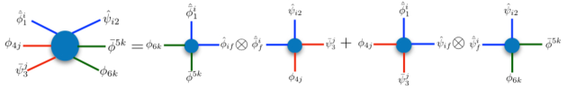
Figure 3: BCFW recursion for the six point amplitude. Factorization into two channels. Each four point amplitude on the RHS is on shell. Two adjacent lines with the same color are color contracted. Note that the gray lines in particular represent the BCFW deformed legs.

The recursion formula can be explicitly written as

$$\langle\bar{\phi}_{1}\psi_{2}\bar{\psi}_{3}\phi_{4}\bar{\phi}_{5}\phi_{6}\rangle=$$

$$\biggl{(}z_{a;f}\frac{z_{b;f}^{2}-1}{z_{a;f}^{2}-z_{b;f}^{2}}\langle\hat{\bar{\phi}}_{1}\hat{\phi}_{f}\bar{\phi}_{5}\phi_{6}\rangle_{z_{a;f}}\langle\hat{\bar{\phi}}_{(-f)}\hat{\psi}_{2}\bar{\psi}_{3}\phi_{4}\rangle_{z_{a;f}}$$

$$+(z_{a;f}\leftrightarrow z_{b;f})\biggr{)}\frac{i}{p^{2}_{f}}\bigg{|}_{p_{f}=p_{234}}$$

$$+\biggl{(}z_{a;f}\frac{z_{b;f}^{2}-1}{z_{a;f}^{2}-z_{b;f}^{2}}\langle\hat{\bar{\phi}}_{1}\hat{\psi}_{f}\bar{\psi}_{3}\phi_{4}\rangle_{z_{a;f}}\langle\hat{\bar{\psi}}_{(-f)}\hat{\psi}_{2}\bar{\phi}_{5}\phi_{6}\rangle_{z_{a;f}}$$

$$+(z_{a;f}\leftrightarrow z_{b;f})\biggr{)}\frac{i}{p^{2}_{f}}\bigg{|}_{p_{f}=p_{256}},$$ (17)

$$= \pqty{\frac{32\pi^{2}i}{\kappa^{2}}}\Bigg{[}\frac{\langle 2|p_{4}|3\rangle\,p_{12}\cdot p_{56}-\langle 2|p_{1}|3\rangle\,p_{34}\cdot p_{56}}{p^{2}_{256}\;p^{2}_{124}}$$

$$+\Bigg{(}\langle 3|p_{12}|5\rangle\,\Big{(}\langle 2|p_{1}|5\rangle\,p_{34}\cdot p_{56}-\langle 2|p_{6}|5\rangle\,p_{34}\cdot p_{12}\Big{)}$$

$$\quad-\langle 34\rangle\langle 12\rangle\,\Big{(}\langle 1|p_{6}|4\rangle\,p_{12}\cdot p_{56}-\langle 1|p_{2}|5\rangle\,\langle 4|p_{6}|5\rangle\Big{)}\Bigg{)}$$

$$\qquad\qquad\qquad\times\frac{1}{p^{2}_{234}\;p^{2}_{123}\;p^{2}_{126}}\Bigg{]}.$$ (18)

Fields with hats corresponds to deformed momenta. We have checked (V) explicitly by computing the relevant Feynman diagrams. It is a curious fact that, the total number of Feynman graphs that contribute to $A_{6}$ is 15. Of these, eleven are reproduced by the channel $p_{f}=p_{234}$ and the remaining four in the channel $p_{f}=p_{256}$. Moreover, we have also reproduced the correct additional poles in the respective channels. The final answer is manifestly free of any spurious poles and square-roots as we argued above.

VI Recursion Relations in the fermionic Theory

In this section, we show that the BCFW recursion relations can be used to compute $2n-$point amplitude $A_{2n}=({\bar{\psi}_{1}}\psi_{2})\cdots({\bar{\psi}_{2n-1}}\psi_{2n})$ for the regular fermionic theory coupled to CS gauge field (1). If we apply (8) to this amplitude, it is easy to show that, it does not have a good large $z$ (as well as $z\rightarrow 0$) behavior, hence we cannot readily apply the BCFW recursion relation to determine all higher point fermionic amplitudes. However, we show below that we can use the recursion relation of the ${\mathcal{N}}=2$ to write a recursion relation for the fermionic theory.

As a first step towards this, let us note that the Feynman diagrams for any tree-level all-fermion scattering amplitude in the $\mathcal{N}=2$ theory (II) is identical to that of the tree-level scattering amplitude in the fermionic theory (1). In the previous section we proved for the $\mathcal{N}=2$ theory that an arbitrary higher-point super-amplitude can be written only in terms of the 4-point super-amplitude. Same can be said for the component amplitudes including the purely fermionic component amplitude . Let us note that for the four point super-amplitude, supersymmetry relates all the component 4-point amplitudes to one component amplitude, which can be taken to be 4-fermion scattering amplitude (see (7)). Thus an arbitrary higher-point component amplitude can be written only in terms of 4-fermion amplitude. This can be recursively done for an arbitrary $2n$ point amplitude, however for simplicity we write the recursion relation for the six point amplitude below

$$\langle\bar{\psi}_{1}\psi_{2}\bar{\psi}_{3}\psi_{4}\bar{\psi}_{5}\psi_{6}\rangle=$$

$$\Biggr{(}z_{a;f}\frac{z_{b;f}^{2}-1}{z_{a;f}^{2}-z_{b;f}^{2}}\quantity[\frac{z_{a;f}^{2}+1}{2z_{a;f}}+i\;\frac{z_{a;f}^{2}-1}{2z_{a;f}}\;\frac{\langle\hat{1}4\rangle}{\langle\hat{f}4\rangle}\frac{\langle\hat{f}6\rangle}{\langle\hat{2}6\rangle}]$$

$$\hskip 85.35826pt\times\langle{\hat{\bar{\psi}}}_{1}{\hat{\psi}}_{f}\bar{\psi}_{3}\psi_{4}\rangle\langle{\hat{\bar{\psi}}}_{(-f)}{\hat{\psi}}_{2}\bar{\psi}_{5}\psi_{6}\rangle_{z_{a;f}}$$

$$+(z_{a;f}\leftrightarrow z_{b;f})\Biggr{)}\frac{1}{p_{f}^{2}}\bigg{|}_{p_{f}=p_{256}}$$

$$+ \Biggr{(}z_{a;f}\frac{z_{b;f}^{2}-1}{z_{a;f}^{2}-z_{b;f}^{2}}\quantity[\frac{z_{a;f}^{2}+1}{2z_{a;f}}+i\;\frac{z_{a;f}^{2}-1}{2z_{a;f}}\;\frac{\langle\hat{1}6\rangle}{\langle\hat{f}6\rangle}\frac{\langle\hat{f}4\rangle}{\langle\hat{2}4\rangle}]$$

$$\hskip 85.35826pt\times\langle{\hat{\bar{\psi}}}_{1}{\hat{\psi}}_{f}\bar{\psi}_{5}\psi_{6}\rangle\langle{\hat{\bar{\psi}}}_{(-f)}{\hat{\psi}}_{2}\bar{\psi}_{3}\psi_{4}\rangle_{z_{a;f}}$$

$$+(z_{a;f}\leftrightarrow z_{b;f})\Biggr{)}\frac{1}{p_{f}^{2}}\bigg{|}_{p_{f}=p_{234}},$$

$$= \pqty{\frac{16\pi^{2}i}{\kappa^{2}}}\pqty{\frac{1}{p_{124}^{2}\;p_{125}^{2}\;p_{256}^{2}}-\frac{1}{p_{123}^{2}\;p_{126}^{2}\;p_{234}^{2}}}\times$$

$$\Bigg{[}-\langle 1|p_{34}|2\rangle\,\langle 3|p_{56}|4\rangle\,\langle 5|p_{12}|6\rangle+\langle 56\rangle\langle 12\rangle\langle 34\rangle\times$$

$$\Big{(}\langle 5|p_{12}|6\rangle\,\langle 56\rangle+\langle 3|p_{56}|4\rangle\,\langle 34\rangle+\langle 1|p_{34}|2\rangle\,\langle 12\rangle\Big{)}\Bigg{]}.$$ (19)

The above answer is remarkably simple and is manifestly invariant under the permutations of particle pairs, $\{12\},\{34\}$ and $\{56\}$, as expected.

VII Discussion

In this letter we presented recursion relations for all tree level amplitudes in $\mathcal{N}=2$ CS matter theory and CS theory coupled to regular fermions. Below we discuss some interesting open questions for future research.

It was shown in Inbasekar et al. (2015), that the $2\rightarrow 2$ scattering amplitude in the ${\mathcal{N}}=2$ theory does not get renormalized except in the anyonic channel, where it gets renormalized by a simple function of the ’t Hooft coupling. A natural question is, why in the $\mathcal{N}=2$ theory the scattering amplitude has such a simple form, whereas the corresponding amplitudes in the fermionic Jain et al. (2015) and other less susy ${\mathcal{N}}=1$ Inbasekar et al. (2015) theories are quite complicated; and, if the simplicity of the amplitudes continues to persist with higher point amplitudes. It is also interesting to explore an analog of the Aharonov-Bohm phase for higher point amplitudes. It may very well turn out that the Aharanov-Bohm phases of higher point amplitudes are products of the Aharonov-Bohm phases of the $2\to 2$ amplitude. BCFW recursion relations provide a strong indication towards this result.

To answer the above questions, we need to compute higher scattering amplitudes to all orders in $\lambda$. A possible way is to investigate the Schwinger-Dyson equation. However, the Schwinger-Dyson equation approach is quite complicated even at the $6$-point level. A refined approach might be to look for a larger class of symmetries such as dual superconformal symmetry Inbasekar et al. (2017), Yangian symmetry and use the powerful formulation of Arkani-Hamed et al. (2016) to obtain results. Given the fact that, these theories are exactly solvable at large-$N$ as well as the fact that ${\mathcal{N}}=2$ theory is self-dual, it could turn out that the ${\mathcal{N}}=2$ theory may be one of the simplest playing grounds to develop new techniques in computing S-matrices to all orders Arkani-Hamed et al. (2016). Furthermore exact solvability at large $N$ indicates that these models might even be integrable. One possible way to investigate integrability is to show the existence of an infinite dimensional Yangian symmetry. Since these theories relate to various physical situations, any of the above exercises may provide insight into finite $N,\kappa$ computations.

Acknowledgements: We thank O. Aharony, S. Ananth, S.Banerjee, R. Gopakumar, Nima Arkani Hamed, T. Hartman, Y-t. Huang, S. Kundu, R. Loganayagam, J. Maldacena, G. Mandal, S. Minwalla, S. Mukhi, S. Raju, A. Sever, T. Sharma, R. Soni, J. Sonnenschein, S. Trivedi, and S. Wadia for helpful discussions. We would like to thank Nima Afkhami-Jeddi and Amirhossein Tajdini for collaboration during the initial stages of the project. We would like to thank Y-t. Huang for sharing a useful mathematica code with us. Special thanks S. Minwalla for very useful and critical discussions. The work of KI was supported in part by a center of excellence supported by the Israel Science Foundation (grant number 1989/14), the US-Israel bi-national fund (BSF) grant number 2012383 and the Germany Israel bi-national fund GIF grant number I-244-303.7-2013. S.J. would like to thank TIFR for hospitality at various stages of the work. Some part of the work in this paper was completed while SJ was a postdoc at Cornell and his research was supported by grant No:488643 from the Simons Foundation. The work of PN is supported partly by Infosys Endowment for the study of the Quantum Structure of Space Time and Indo-Israel grant of S. Minwalla; and partly by the College of Arts and Sciences of the University of Kentucky. We would also like to thank people of India for their steady support in basic research.

VIII Appendix

VIII.1 Large $z$ behavior of the six point scattering amplitude $(\bar{\phi}(p_{1})\psi(p_{2}))(\bar{\psi}(p_{3})\phi(p_{4}))(\bar{\phi}(p_{5})\phi(p_{6}))$

In this section, we compute the six point scattering amplitude $\quantity(\bar{\phi}(p_{1})\psi(p_{2}))\quantity(\bar{\psi}(p_{3})\phi(p_{4}))\quantity(\bar{\phi}(p_{5})\phi(p_{6}))$ and demonstrate that it is well behaved under the BCFW deformations. The Feynman diagrams that contribute to the six point function under consideration are displayed in fig 4.

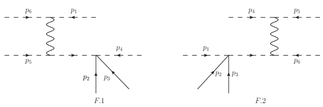
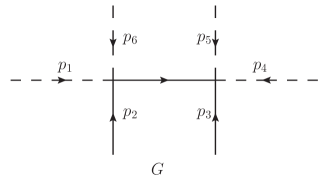
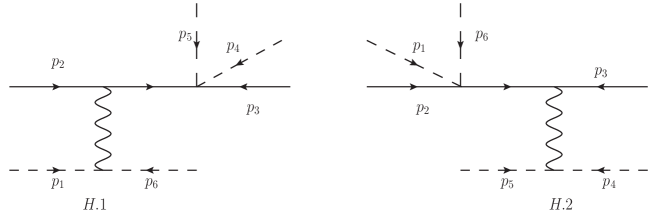
Figure 4: Feynman diagrams for the amplitude $(\bar{\phi}(p_{1})\psi(p_{2}))(\bar{\psi}(p_{3})\phi(p_{4}))(\bar{\phi}(p_{5})\phi(p_{6}))$

We give below explicit expression for each diagram appearing in Fig.4

$$A_{1}= -\frac{16\pi^{2}i}{\kappa^{2}}\frac{p_{1}.(p_{2}-p_{3})}{p_{23}^{2}p_{45}^{2}p_{123}^{2}}\langle 23\rangle\langle 45\rangle\langle 56\rangle\langle 46\rangle$$ (20)

$$A_{2}= \frac{16\pi^{2}i}{\kappa^{2}}\frac{p_{4}.(p_{2}-p_{3})}{p_{23}^{2}p_{16}^{2}p_{234}^{2}}\langle 23\rangle\langle 16\rangle\langle 65\rangle\langle 15\rangle$$ (21)

$$A_{3}= \frac{4i\pi^{2}}{\kappa^{2}}\frac{\langle 16\rangle\langle 45\rangle}{p_{16}^{2}p^{2}_{45}p^{2}_{126}}\left(\langle 21\rangle(\langle 34\rangle\langle 5|p_{12}|6\rangle+\langle 35\rangle\langle 6|p_{12}|4\rangle)+\langle 26\rangle(\langle 34\rangle\langle 1|p_{26}|5\rangle+\langle 35\rangle\langle 1|p_{26}|4\rangle)\right)$$ (22)

$$B_{1}= \frac{8\pi^{2}i}{\kappa^{2}}\langle 14\rangle\left(\frac{\langle 1|p_{56}|3\rangle\langle 24\rangle+\langle 3|p_{56}|4\rangle\langle 21\rangle}{p_{14}^{2}p_{356}^{2}}\right)$$ (23)

$$B_{2}= \frac{8\pi^{2}i}{\kappa^{2}}\langle 14\rangle\left(\frac{\langle 1|p_{56}|2\rangle\langle 34\rangle+\langle 2|p_{56}|4\rangle\langle 31\rangle}{p_{14}^{2}p_{256}^{2}}\right)$$ (24)

$$C_{1}= -\frac{8\pi^{2}i}{\kappa^{2}}\left(\frac{\langle 2|p_{1}|3\rangle(p_{23}.p_{6})-\langle 2|p_{6}|3\rangle(p_{23}.p_{1})}{p^{2}_{23}p^{2}_{16}}\right)$$ (25)

$$C_{2}= -\frac{8\pi^{2}i}{\kappa^{2}}\left(\frac{\langle 2|p_{5}|3\rangle(p_{23}.p_{4})-\langle 2|p_{4}|3\rangle(p_{23}.p_{5})}{p^{2}_{23}p^{2}_{45}}\right)$$ (26)

$$D_{1}= \frac{8\pi^{2}i}{\kappa^{2}}\frac{\langle 2|p_{14}|3\rangle}{p_{124}^{2}}$$ (27)

$$D_{2}= \frac{8\pi^{2}i}{\kappa^{2}}\frac{\langle 2|p_{56}|3\rangle}{p_{256}^{2}}$$ (28)

$$E= -\frac{4\pi^{2}i}{\kappa^{2}}\langle 45\rangle\langle 23\rangle\left(\frac{(\langle 12\rangle^{2}-\langle 13\rangle^{2})\langle 46\rangle\langle 56\rangle-(\langle 26\rangle^{2}-\langle 36\rangle^{2})\langle 14\rangle\langle 15\rangle}{p_{23}^{2}p_{45}^{2}p_{16}^{2}}\right)$$ (29)

$$F_{1}= \frac{8\pi^{2}i}{\kappa^{2}}\frac{\langle 23\rangle\langle 16\rangle\langle 65\rangle\langle 15\rangle}{p^{2}_{16}p^{2}_{234}}$$ (30)

$$F_{2}= \frac{8\pi^{2}i}{\kappa^{2}}\frac{\langle 23\rangle\langle 45\rangle\langle 56\rangle\langle 46\rangle}{p^{2}_{45}p^{2}_{231}}$$ (31)

$$G= \frac{4\pi^{2}i}{\kappa^{2}}\frac{\langle 2|p_{16}|3\rangle}{p_{126}^{2}}$$ (32)

$$H_{1}= \frac{4\pi^{2}i}{\kappa^{2}}\langle 16\rangle\left(\frac{\langle 12\rangle\langle 6|p_{12}|3\rangle-\langle 26\rangle\langle 1|p_{26}|3\rangle}{p_{16}^{2}p_{126}^{2}}\right)$$ (33)

$$H_{2}= -\frac{4\pi^{2}i}{\kappa^{2}}\langle 45\rangle\left(\frac{\langle 35\rangle\langle 2|p_{16}|4\rangle+\langle 34\rangle\langle 2|p_{16}|5\rangle}{p^{2}_{45}p^{2}_{126}}\right)$$ (34)

It is easy to verify that the the asymptotic behavior of the full set of diagram is well behaved by deforming the momentum $p_{1}$ and $p_{2}$, as discussed in section III and IV. We apply the BCFW deformations in the large z limit using

$$p_{2} \to qz^{2}$$ (35)

$$p_{1} \to-qz^{2}\$$ (36)

and obtain the asymptotic behavior of the amplitudes to leading order in $z$ as follows. The diagrams $A_{2},C_{1},D_{2},F_{1}$ in (4) go as $O(1/z)$ to the leading order in the large z limit.

$$A_{2}\sim \frac{2\pi^{2}i}{\kappa^{2}z}\frac{(q.p_{4})\langle q3\rangle\langle q6\rangle\langle 65\rangle\langle q5\rangle}{(q.p_{3})(q.p_{34})(q.p_{6})}+\mathcal{O}\quantity(\frac{1}{z^{3}})$$ (37)

$$B_{2}\sim \frac{2\pi^{2}i}{\kappa^{2}z}\frac{\langle q4\rangle(\langle q|p_{56}|q\rangle\langle 34\rangle+\langle q|p_{56}|4\rangle\langle 3q\rangle)}{(q.p_{4})(q.p_{56})}+\mathcal{O}\quantity(\frac{1}{z^{3}})$$ (38)

$$C_{1}\sim \frac{2\pi^{2}i}{\kappa^{2}z}\frac{\langle q|p_{6}|3\rangle}{(q.p_{6})}+\mathcal{O}\quantity(\frac{1}{z^{3}})$$ (39)

$$D_{2}\sim \frac{4\pi^{2}i}{\kappa^{2}z}\frac{\langle q|p_{56}|3\rangle}{q.p_{56}}+\mathcal{O}\quantity(\frac{1}{z^{3}})$$ (40)

$$F_{1}\sim \frac{2\pi^{2}i}{\kappa^{2}z}\frac{\langle q3\rangle\langle q6\rangle\langle 65\rangle\langle q5\rangle}{(q.p_{6})(q.p_{34})}+\mathcal{O}\quantity(\frac{1}{z^{3}})$$ (41)

For the remaining diagrams we just display the leading large $z$ behavior. They are given by

$$A_{1}\sim-\frac{8\pi^{2}iz}{\kappa^{2}}\frac{\langle q3\rangle\langle 45\rangle\langle 56\rangle\langle 46\rangle}{p_{45}^{2}p^{2}_{123}}+{\mathcal{O}}\quantity(\frac{1}{z}) F_{2}\sim\frac{8\pi^{2}iz}{\kappa^{2}}\frac{\langle q3\rangle\langle 45\rangle\langle 56\rangle\langle 46\rangle}{p_{45}^{2}p^{2}_{123}}+{\mathcal{O}}\quantity(\frac{1}{z})$$ (43)

$$B_{1}\sim\frac{8\pi^{2}iz}{\kappa^{2}}\frac{\langle q|p_{56}|3\rangle}{p_{356}^{2}}+{\mathcal{O}}\quantity(\frac{1}{z})\ \ D_{1}\sim-\frac{8\pi^{2}iz}{\kappa^{2}}\frac{\langle q|p_{56}|3\rangle}{p_{356}^{2}}+{\mathcal{O}}\quantity(\frac{1}{z})$$ (44)

$$A_{3}\sim-\frac{4\pi^{2}iz}{\kappa^{2}}\frac{\langle 45\rangle(\langle 34\rangle\langle q|p_{34}|5\rangle+\langle 35\rangle\langle q|p_{35}|4\rangle)}{p^{2}_{45}p^{2}_{126}}+{\mathcal{O}}\quantity(\frac{1}{z}) H_{2}\sim\frac{4\pi^{2}iz}{\kappa^{2}}\frac{\langle 45\rangle(\langle 34\rangle\langle q|p_{34}|5\rangle+\langle 35\rangle\langle q|p_{35}|4\rangle)}{p^{2}_{45}p^{2}_{126}}+{\mathcal{O}}\quantity(\frac{1}{z})$$ (45)

$$C_{2}\sim\frac{2\pi^{2}iz}{\kappa^{2}}\frac{\langle q4\rangle\langle q5\rangle\langle 3q\rangle\langle 45\rangle}{p^{2}_{45}(q.p_{3})}+{\mathcal{O}}\quantity(\frac{1}{z}) E\sim-\frac{2\pi^{2}iz}{\kappa^{2}}\frac{\langle q4\rangle\langle q5\rangle\langle 3q\rangle\langle 45\rangle}{p^{2}_{45}(q.p_{3})}+{\mathcal{O}}\quantity(\frac{1}{z})$$ (46)

$$G\sim-\frac{4\pi^{2}iz}{\kappa^{2}}\frac{\langle q|p_{45}|3\rangle}{p^{2}_{126}}+{\mathcal{O}}\quantity(\frac{1}{z}) H_{1}\sim\frac{4\pi^{2}iz}{\kappa^{2}}\frac{\langle q|p_{45}|3\rangle}{p^{2}_{126}}+{\mathcal{O}}\quantity(\frac{1}{z})$$ (47)

Even though some of the individual diagrams are divergent linearly in $z$, the divergences in the total amplitude cancel pair wise in the large $z$ limit as is evident from the way we have written the results. For example linear in $z$ behavior cancelling pair wise in $\left(A_{1},F_{2}\right),~{}(B_{1},D_{1})$ etc. Thus the total amplitude is well behaved as $z\to\infty$. A straightforward computation yields the analogous result for the $z\to 0$ limit. Thus the amplitude $A_{6}\quantity((\bar{\phi}(p_{1})\psi(p_{2}))(\bar{\psi}(p_{3})\phi(p_{4}))(\bar{\phi}(p_{5})\phi(p_{6})))$ is well behaved under the BCFW deformations both at $z\to\infty$ and $z\to 0$.

Towards the end of §V we had mentioned that four of the diagrams are reproduced in the factorization channel $p_{f}=p_{256}$, these diagrams are $B_{1},B_{2},D_{1},D_{2}$ in fig 4. The remaining eleven diagrams in fig 4 are reproduced in the factorization channel $p_{f}=p_{234}$.

VIII.2 A Dyson-Schwinger equation for all loop six point correlator

As we saw earlier, the basic building block of higher point amplitudes in the Chern-Simons matter theories at the tree level is the four point amplitude. In this section we describe the Dyson-Schwinger construction of the all loop six point correlator

$$\langle\bar{\Phi}^{i}(p+q,\theta_{1})\Phi_{i}(-p,\theta_{2})\bar{\Phi}^{j}(k+q^{\prime},\theta_{3})\Phi_{j}(-k-q,\theta_{6})\bar{\Phi}^{k}(r,\theta_{5})\Phi_{k}(-r-q^{\prime},\theta_{4})\rangle$$ (48)

using the superspace Schwinger-Dyson construction developed in Inbasekar et al. (2015). In the above $\Phi^{i}$ is a complex scalar superfield in $\mathcal{N}=1$ superspace defined by

$$\Phi^{i}=\phi^{i}+\theta\psi^{i}-\theta^{2}F^{i}$$ (49)

where $\phi^{i}$ is a complex scalar, $\psi^{i}$ is a complex fermion and $F^{i}$ is a complex auxiliary field. The $\mathcal{N}=2$ theory can be written in $\mathcal{N}=1$ superspace in terms of $\Phi^{i}$. For more details see Inbasekar et al. (2015). Before presenting the central idea it is informative to understand the color structure of the tree level and one loop amplitudes in the theory. In the supersymmetric Light cone gauge these are described succinctly in fig 5 and in fig 6.

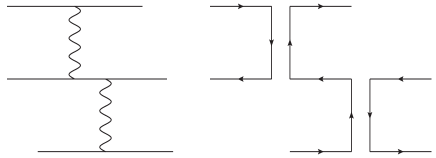
Figure 5: Six point correlator: We display tree diagrams in supersymmetric light cone gauge. For simplicity we have only displayed the ladder diagrams.The tree diagrams are of order ${\mathcal{O}}(\frac{1}{\kappa^{2}})$ since the gauge field propagator contributes a factor of ${\mathcal{O}}(\frac{1}{\kappa})$.

It turns out that, there are six different diagrams for a given color contracted correlator. We have displayed only one in Fig.5 for brevity.

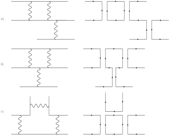
Figure 6: Six point correlator: We have listed the various contributions to the one loop correlator in supersymmetric light cone gauge. For simplicity we have displayed only the ladder diagrams. In fig a) and c) the three gauge field propagators contribute a factor of ${\mathcal{O}}(\frac{1}{\kappa^{3}})$ and the single color loop gives a factor of $N$, leading to a contribution of the order $\frac{\lambda}{\kappa^{2}}$. Note that this is of the same order in $\kappa$ as the tree level diagram displayed in fig 5. On the other hand fig b) has three gauge fields and no color loops, rendering it to be $O(\frac{1}{\kappa^{3}})$.

The situation is a little bit more complicated at one loop as three different type of diagrams can appear as displayed in fig 6. Note that diagrams like fig 6 b) are suppressed in the large $N,\kappa$ limit (keeping $\lambda=\frac{N}{\kappa}$ fixed). So they don’t contribute to the Schwinger-Dyson equation at this order. It can be checked that these type of diagrams continue to remain suppressed at higher loops.

This paves way for the construction of all loop higher point correlators entirely in terms of all-loop four point correlators at least in the planar approximation. The case for the six point correlator is displayed in (see fig 7).

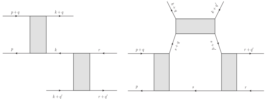
Figure 7: Six point correlator in superspace: The grey boxes represent the $\mathcal{N}=2$ all-loop four point correlator computed in Inbasekar et al. (2015)

It is straightforward to write down the correlator for the first diagram in 7, the second contribution however requires a loop integration over both intermediate grassmann and momentum variables and is quite complicated, we defer a detailed treatment to future works.

References

- Inbasekar et al. (2015) K. Inbasekar, S. Jain, S. Mazumdar, S. Minwalla, V. Umesh, and S. Yokoyama, JHEP 10, 176 (2015), arXiv:1505.06571 [hep-th] .
- Aharony et al. (2012a) O. Aharony, G. GurAri, and R. Yacoby, JHEP 1203, 037 (2012a), arXiv:1110.4382 [hep-th] .
- Giombi et al. (2012) S. Giombi, S. Minwalla, S. Prakash, S. P. Trivedi, S. R. Wadia, and X. Yin, Eur. Phys. J. C72, 2112 (2012), arXiv:1110.4386 [hep-th] .
- Klebanov and Polyakov (2002) I. R. Klebanov and A. M. Polyakov, Phys. Lett. B550, 213 (2002), arXiv:hep-th/0210114 [hep-th] .
- Sezgin and Sundell (2002) E. Sezgin and P. Sundell, Nucl. Phys. B644, 303 (2002), [Erratum: Nucl. Phys.B660,403(2003)], arXiv:hep-th/0205131 [hep-th] .
- Giombi and Yin (2010) S. Giombi and X. Yin, JHEP 09, 115 (2010), arXiv:0912.3462 [hep-th] .
- Maldacena and Zhiboedov (2013a) J. Maldacena and A. Zhiboedov, J.Phys. A46, 214011 (2013a), arXiv:1112.1016 [hep-th] .
- Maldacena and Zhiboedov (2013b) J. Maldacena and A. Zhiboedov, Class.Quant.Grav. 30, 104003 (2013b), arXiv:1204.3882 [hep-th] .
- Aharony et al. (2012b) O. Aharony, G. Gur-Ari, and R. Yacoby, JHEP 1212, 028 (2012b), arXiv:1207.4593 [hep-th] .
- Gur-Ari and Yacoby (2013) G. Gur-Ari and R. Yacoby, JHEP 1302, 150 (2013), arXiv:1211.1866 [hep-th] .
- Gurucharan and Prakash (2014) V. Gurucharan and S. Prakash, JHEP 1409, 009 (2014), arXiv:1404.7849 [hep-th] .
- Bedhotiya and Prakash (2015) A. Bedhotiya and S. Prakash, JHEP 12, 032 (2015), arXiv:1506.05412 [hep-th] .
- GurAri and Yacoby (2015) G. GurAri and R. Yacoby, JHEP 11, 013 (2015), arXiv:1507.04378 [hep-th] .
- Geracie et al. (2016) M. Geracie, M. Goykhman, and D. T. Son, JHEP 04, 103 (2016), arXiv:1511.04772 [hep-th] .
- Gur-Ari et al. (2016) G. Gur-Ari, S. A. Hartnoll, and R. Mahajan, JHEP 07, 090 (2016), arXiv:1605.01122 [hep-th] .
- Jain et al. (2012) S. Jain, S. P. Trivedi, S. R. Wadia, and S. Yokoyama, JHEP 1210, 194 (2012), arXiv:1207.4750 [hep-th] .
- Yokoyama (2013) S. Yokoyama, JHEP 1301, 052 (2013), arXiv:1210.4109 [hep-th] .
- Aharony et al. (2013) O. Aharony, S. Giombi, G. Gur-Ari, J. Maldacena, and R. Yacoby, JHEP 1303, 121 (2013), arXiv:1211.4843 [hep-th] .
- Jain et al. (2013a) S. Jain, S. Minwalla, T. Sharma, T. Takimi, S. R. Wadia, et al., JHEP 1309, 009 (2013a), arXiv:1301.6169 [hep-th] .
- Takimi (2013) T. Takimi, JHEP 1307, 177 (2013), arXiv:1304.3725 [hep-th] .
- Jain et al. (2013b) S. Jain, S. Minwalla, and S. Yokoyama, JHEP 1311, 037 (2013b), arXiv:1305.7235 [hep-th] .
- Yokoyama (2014) S. Yokoyama, JHEP 1401, 148 (2014), arXiv:1310.0902 [hep-th] .
- Minwalla and Yokoyama (2016) S. Minwalla and S. Yokoyama, JHEP 02, 103 (2016), arXiv:1507.04546 [hep-th] .
- Nosaka and Yokoyama (2018) T. Nosaka and S. Yokoyama, JHEP 01, 001 (2018), arXiv:1706.07234 [hep-th] .
- Jain et al. (2015) S. Jain, M. Mandlik, S. Minwalla, T. Takimi, S. R. Wadia, et al., JHEP 1504, 129 (2015), arXiv:1404.6373 [hep-th] .
- Dandekar et al. (2015) Y. Dandekar, M. Mandlik, and S. Minwalla, JHEP 1504, 102 (2015), arXiv:1407.1322 [hep-th] .
- Yokoyama (2016) S. Yokoyama, JHEP 09, 105 (2016), arXiv:1604.01897 [hep-th] .
- Giombi et al. (2017) S. Giombi, V. Gurucharan, V. Kirilin, S. Prakash, and E. Skvortsov, JHEP 01, 058 (2017), arXiv:1610.08472 [hep-th] .
- Wadia (2016) S. R. Wadia, Int. J. Mod. Phys. A31, 1630052 (2016).
- Radicevic et al. (2016) D. Radicevic, D. Tong, and C. Turner, JHEP 12, 067 (2016), arXiv:1608.04732 [hep-th] .
- Giombi (2017) S. Giombi, (2017), arXiv:1707.06604 [hep-th] .
- Radicevic (2016) D. Radicevic, JHEP 03, 131 (2016), arXiv:1511.01902 [hep-th] .
- Aharony (2016) O. Aharony, JHEP 02, 093 (2016), arXiv:1512.00161 [hep-th] .
- Seiberg et al. (2016) N. Seiberg, T. Senthil, C. Wang, and E. Witten, Annals Phys. 374, 395 (2016), arXiv:1606.01989 [hep-th] .
- Karch and Tong (2016) A. Karch and D. Tong, Phys. Rev. X6, 031043 (2016), arXiv:1606.01893 [hep-th] .
- Karch et al. (2017) A. Karch, B. Robinson, and D. Tong, JHEP 01, 017 (2017), arXiv:1609.04012 [hep-th] .
- Hsin and Seiberg (2016) P.-S. Hsin and N. Seiberg, JHEP 09, 095 (2016), arXiv:1607.07457 [hep-th] .
- Aharony et al. (2017) O. Aharony, F. Benini, P.-S. Hsin, and N. Seiberg, JHEP 02, 072 (2017), arXiv:1611.07874 [cond-mat.str-el] .
- Benini et al. (2017) F. Benini, P.-S. Hsin, and N. Seiberg, JHEP 04, 135 (2017), arXiv:1702.07035 [cond-mat.str-el] .
- Gaiotto et al. (2017) D. Gaiotto, Z. Komargodski, and N. Seiberg, (2017), arXiv:1708.06806 [hep-th] .
- Jensen and Karch (2017a) K. Jensen and A. Karch, JHEP 11, 018 (2017a), arXiv:1709.01083 [hep-th] .
- Jensen and Karch (2017b) K. Jensen and A. Karch, JHEP 12, 031 (2017b), arXiv:1709.07872 [hep-th] .
- Gang et al. (2011) D. Gang, Y.-t. Huang, E. Koh, S. Lee, and A. E. Lipstein, JHEP 03, 116 (2011), arXiv:1012.5032 [hep-th] .
- Lipstein and Mason (2013) A. E. Lipstein and L. Mason, JHEP 01, 009 (2013), arXiv:1207.6176 [hep-th] .
- Agarwal et al. (2014) A. Agarwal, A. E. Lipstein, and D. Young, Phys. Rev. D89, 045020 (2014), arXiv:1302.5288 [hep-th] .
- Elvang and Huang (2015) H. Elvang and Y.-t. Huang, Scattering Amplitudes in Gauge Theory and Gravity (Cambridge University Press, 2015).
- Arkani-Hamed and Kaplan (2008) N. Arkani-Hamed and J. Kaplan, JHEP 04, 076 (2008), arXiv:0801.2385 [hep-th] .
- Note (1) For instance, for theory, the Lagrangian for which can be found in Inbasekar et al. (2015) (Equation (2.11)), (13\@@italiccorr) is modified to whereas (12\@@italiccorr) remains the same. Here is a free parameter in theory. This implies that only at , the theory has a good large z behavior. This is exactly the point in the line where the supersymmetry of the theory gets enhanced to .
- Note (2) Although, formula (14\@@italiccorr) looks very similar to ABJM case, the details are different since the external matter particles are in fundamental representation. For example, in general there will be more factorization channels here as compared to the ABJM case. For example, in the six point function, as will be clear below, there are two factorized channels, where as for the corresponding deformation in ABJM, there is only one factorized channel.
- Note (3) Under , both and (see (8\@@italiccorr) and (9\@@italiccorr)). From (4\@@italiccorr) one can deduce that the scaling of the onshell fields to be under . In our BCFW deformations, we deform one and one , and therefore, . See Gang et al. (2011) for a related discussion in the context of the ABJM theory.
-
Note (4)
A general six point super amplitude in theory can be written in terms of two independent functions as
where as defined in (5\@@italiccorr). - Note (5) There will be some non-trivial boundary terms that do not vanish and in general there are no good prescriptions to compute them systematically.
- Note (6) Note that the recursion relation in the theory (14\@@italiccorr) does not directly give in terms of the lower point fermionic amplitude. However, we can use BCFW relations recursively to write down any higher point amplitude in terms of four point amplitudes such as , , , etc. Moreover, at the level of the four point amplitude, one can rewrite this in terms of . For example, . This implies that we get a recursion relation for in terms of lower point fermionic amplitudes only. Hence this can be interpreted as a BCFW recursion relation in the regular fermionic theory coupled to CS gauge field (1\@@italiccorr).
- Inbasekar et al. (2017) K. Inbasekar, S. Jain, S. Majumdar, P. Nayak, T. Neogi, T. Sharma, R. Sinha, and V. Umesh, (2017), arXiv:1711.02672 [hep-th] .
- Arkani-Hamed et al. (2016) N. Arkani-Hamed, J. L. Bourjaily, F. Cachazo, A. B. Goncharov, A. Postnikov, and J. Trnka, Grassmannian Geometry of Scattering Amplitudes (Cambridge University Press, 2016) arXiv:1212.5605 [hep-th] .