PYROOMACOUSTICS: A PYTHON PACKAGE FOR AUDIO ROOM SIMULATION AND ARRAY PROCESSING ALGORITHMS

Abstract

We present pyroomacoustics, a software package aimed at the rapid development and testing of audio array processing algorithms. The content of the package can be divided into three main components: an intuitive Python object-oriented interface to quickly construct different simulation scenarios involving multiple sound sources and microphones in 2D and 3D rooms; a fast C implementation of the image source model for general polyhedral rooms to efficiently generate room impulse responses and simulate the propagation between sources and receivers; and finally, reference implementations of popular algorithms for beamforming, direction finding, and adaptive filtering. Together, they form a package with the potential to speed up the time to market of new algorithms by significantly reducing the implementation overhead in the performance evaluation step.

Index Terms—  RIR, simulation, rapid prototyping, reference implementations, reproducibility

1 Introduction

As in all engineering disciplines, objective evaluation of new (array) audio processing algorithms is essential to the assessment of their value. The gold standard for such evaluation is to design and carry out an experiment in a controlled environment with a real microphone array and careful calibration of the locations of all sound sources. The time and effort needed to setup these experiments naturally limit the number of replications of the experiments and the number of scenarios that can be explored. In the exploratory phase of research, numerical simulation is an attractive alternative. It allows one to quickly test and iterate a large number of ideas. In addition it makes it possible to finely tune parameters for the algorithm before going to experiments in the physical world.

There are typically three components in a simulation system. First, a programming language to describe the scenarios to simulate. Second, a computer program implementing a model that simulates the relevant physical effects, in our case the propagation of sound in air. Finally, we need computer programs implementing the algorithms under investigation.

While low level languages like C and FORTRAN are the most efficient when it comes to speed, they come at a significant cost in terms of implementation complexity. High level scripting languages have long been a popular alternative for describing simulations. In particular, MATLAB has been historically the industry, and often academic, standard for signal processing numerical experiments. Its high level syntax based on linear algebraic operations is indeed particularly well suited for algorithms in this field. It comes however with significant drawbacks: high cost, closed source, and a clunky syntax for anything other than linear algebra. In recent years Python has come to prominence as an attractive alternative to MATLAB for high level scientific computing [1]. Its focus on code readability and extensibility makes it a candidate of choice for reproducible scientific code [2]. The numpy and scipy modules extend Python with the same powerful linear algebra primitives that MATLAB enjoys. An aspect of special interest for DSP engineers is the massive adoption of Python in the machine learning community as exemplified by the scikit-learn [3] or speech recognition packages [4]. Finally, Python is a community supported free and open source project that includes robust tools for distribution (http://pypi.python.org), documentation (http://readthedocs.io), and continuous integration (http://travis-ci.org).

For a simulation to yield useful information and practical insight, it is vital that it models accurately enough real conditions. In room acoustics, simulation based on the image source model (ISM) has been used extensively for this purpose and has well-known strengths and weaknesses [5]. This model replaces reflections on walls by virtual sources playing the same sound as the original source and builds a room impulse response (RIR) from the corresponding delays and attenuations. Its strength is its simplicity. The model is accurate only as long as the wavelength of the sound is small relative to the size of the reflectors, which it assumes to be uniformly absorbing across frequencies. Nevertheless, these assumptions are not too far from reality in many environments of interests such as offices. The original model can be extended to convex and non-convex polyhedral rooms in two and three dimensions [6]. Our wishlist for an RIR generator is: affordable, open source, and flexible. A number of generators are available, and most if not all are shared online free of charge, e.g. the popular generator from Emanuël Habets [7]. Unfortunately, none allow room shapes other than rectangular. Furthermore, most rely on MATLAB. Faced by the limitations of available RIR generators, we decided to develop our own.

We provide pyroomacoustics, a comprehensive Python package for audio algorithms simulation. The package includes both a fast RIR generator based on the ISM and a number of reference implementations of popular algorithms for beamforming, direction of arrival (DOA) finding, and adaptive filtering. A short time Fourier transform (STFT) engine allows for efficient frequency domain processing. The object oriented features of Python are used to provide a LEGO-like interface to these different blocks. This paper gives an overview of the usage and content of pyroomacoustics. The software itself is available under a permissive open source license through the standard Python package manager or on github.

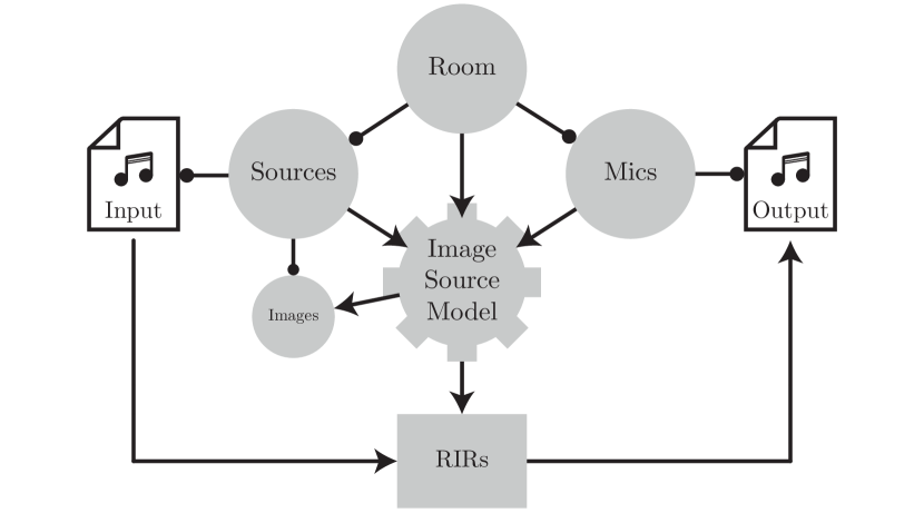
Fig. 1: Structure of the sound propagation simulator. The lines terminated by a bullet indicate attribute relationship. Arrows indicates parameters to functions.

2 Pyroomacoustics Core

The pyroomacoustics package exploits the object oriented features of Python to create a clean and intuitive application programming interface (API) for room acoustics simulation. The three main classes are Room, SoundSource, and MicrophoneArray. On a high level, a simulation scenario is created by first defining a room to which a few sound sources and a microphone array are attached. The actual audio is attached to the source as a raw audio sample. The ISM is then used to find all image sources up to a maximum specified order and RIRs are generated from their positions. The RIR generator is described in more details in Section 3. The microphone signals are then created by convolving the audio samples associated to sources with the appropriate RIR. Since the simulation is done on discrete-time signals, a sampling frequency is specified for the room and the sources it contains. Microphones can optionally operate at a different sampling frequency; a rate conversion is done in this case. A simple code example and its output are shown in Figure 4.

2.1 The Room Class

A Room object has as attributes a collection of Wall objects, a microphone array, and a list of sound sources. The room can be two dimensional (2D), in which case the walls are simply line segments. A factory method from_corners can be used to create the room from a polygon. In three dimensions (3D), the walls are two dimensional polygons, namely a collection of points lying on a common plane. Creating rooms in 3D is more tedious and for convenience a method extrude is provided to lift a 2D room into 3D space by adding vertical walls and a parallel “ceiling” (see Figure 4b). The Room is sub-classed by ShoeBox which creates a rectangular (2D) or parallelepipedic (3D) room. As will be detailed in Section 3, such rooms benefit from an efficient algorithm for the ISM.

2.2 The SoundSource Class

A SoundSource object has as attributes the locations of the source itself and also all of its image sources. This list is usually generated by the Room object containing the source. The reason for this structure is to anticipate scenarios where the room is defined by the locations of the image sources, for example in room inference problems [8]. The source object also contains the methods to build an RIR from the image sources locations. The image sources are conveniently available through the overloaded bracket operator. This comes handy to select only a subset of image sources, such as when building acoustic rake receivers [9].

2.3 The MicrophoneArray and Beamformer Classes

The MicrophoneArray class is essentially an array of microphone locations together with a sampling frequency. It has in addition a record method that wraps potential rate conversions when the simulation and microphones are at different rates.

The Beamformer class inherits from MicrophoneArray and can be used instead. In that case, beamforming weights (in the frequency domain) or filters (in the time domain) can be computed according to several methods (see Section 4.1). Figure 5 shows an example of a delay-and-sum (DS) beamformer in a rectangular room.

In addition, the Beamformer class packs an STFT engine for efficient frame processing in the frequency domain (see Figure 2). The engine allows for variable size zero-padding, overlap, and the use of different analysis and synthesis windows. Alternatively, direct filtering in the time domain is also possible. Specialized methods can convert weights to a corresponding filter and vice-versa. In case of mismatch in size, a least squares fit of the beamforming weights to a smaller filter is done.

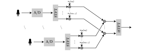
Fig. 2: Block diagram of STFT domain beamforming.

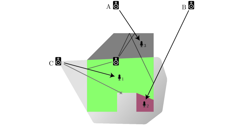
Fig. 3: Image source model for arbitrary polyhedral rooms. Sources A and B are visible from all microphones. Source C is only visible in the shaded/green area due to the obtuse angle. Microphone 2 is hidden due to obstruction by a re-entrant wall.

3 Room Impulse Response Generator

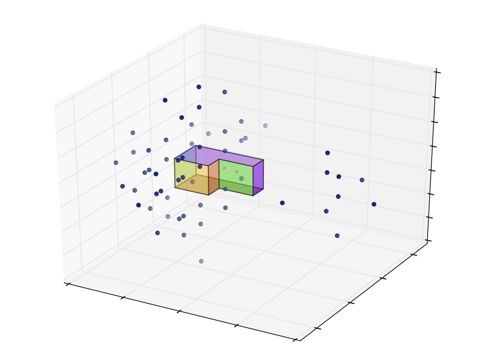
(a) The room

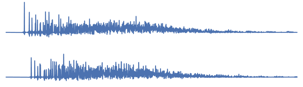
(b) The RIRs

⬇

1import numpy as np

2import matplotlib.pyplot as plt

3import pyroomacoustics as pra

4

5# Create a 2D room from the corners of a polygon

6floor = np.array([[0, 0, 6, 6, 3, 3], # x-coordinates

7 [0, 3, 3, 1.5, 1.5, 0]]) # y-coordinates

8room = pra.Room.from_corners(floor, fs=16000,

9 max_order=12, absorption=0.1)

10

11# Lift the room in 3D space

12room.extrude(2.4)

13

14# Add a sound source

15room.add_source([1.5, 1.2, 1.6])

16

17# Place two microphones in the room

18R = np.array([[3., 4.2], [2.25, 2.1], [1.4, 1.4]])

19bf = pra.MicrophoneArray(R, room.fs)

20room.add_microphone_array(bf)

21

22# Run image source model and show room and 2nd order images

23room.image_source_model()

24room.plot(img_order=3, aspect=’equal’)

25

26fig = plt.figure()

27room.plot_rir()

28plt.show()

(c) Python code to generate these figures

Fig. 4: (a) An example of a non-convex room containing one source and two microphones with up to 3rd order image sources drawn. (b) The two RIRs between the source and the microphones produced by pyroomacoustics. (c) The Python code used to generate the first two figures.

The RIR generator is based on the ISM and considers two cases: shoe box, i.e. rectangular, and arbitrary polyhedral rooms. For shoe box rooms, the original algorithm from Allen and Berkley [5] is used. In this case, symmetries limit the number of image sources to grow quadratically and cubically in 2D and 3D, respectively, in the order of reflections. In addition, image sources are always visible from anywhere in the room. The situation for arbitrary polyhedral rooms is not that simple. The number of image sources grows exponentially in the order of reflections and the visibility of sources must be checked. When obtuse angles occur between walls, the reflections from these walls will not be visible in the whole room. In addition, if the room is not convex, i.e. re-entrant walls occur, they might obstruct the path between image sources and microphones. Both situations are illustrated in Figure 3. The algorithm is explained in detail in the original paper by Borish [6]. In practice, we found its pure Python implementation to be too slow to be practical and hence moved to compiled C code for that part of the package.

Once the location of image sources and their visibility from each microphone is determined, they can be used to construct the RIRs themselves. For a microphone placed at $\bm{r}$, a real source $\bm{s}_{0}$, and a set of its visible image sources $\mathcal{V}_{\bm{r}}(\bm{s}_{0})$, the impulse response between $\bm{r}$ and $\bm{s}_{0}$, sampled at $F_{s}$, is given by

$$a_{\bm{r}}(\bm{s}_{0},n)=\sum_{\bm{s}\in\mathcal{V}_{\bm{r}}(\bm{s}_{0})}\frac{(1-\alpha)^{\text{gen}(\bm{s})}}{4\pi\|\bm{r}-\bm{s}\|}\,\delta_{\text{LP}}\left(n-F_{s}\frac{\|\bm{r}-\bm{s}\|}{c}\right),$$ (1)

where $\text{gen}(\bm{s})$ gives the reflection order of source $\bm{s}$, $\alpha\in[0,1]$ is the absorption factor of the walls, $c$ is the speed of sound, and $\delta_{\text{LP}}$ is the windowed sinc function

$$\delta_{\text{LP}}(t)=\begin{cases}\frac{1}{2}\left(1+\cos\left(\frac{2\pi{t}}{T_{w}}\right)\right)\operatorname{sinc}(t)&\text{if $-\frac{T_{w}}{2}\leq t\leq\frac{T_{w}}{2}$,}\\ 0&\text{otherwise.}\end{cases}$$ (2)

The parameter $T_{w}$ controls the width of the window and thus the degree of approximation to a full sinc. Note that for simplicity we assumed the absorption factor to be identical for all walls. Nevertheless, the package allows to specify a different absorption factor for each wall. Two RIRs produced this way can be seen in Figure 4b.

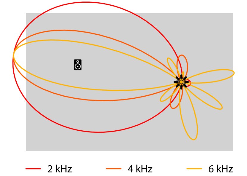
(a) DS Beamformer

⬇

1import numpy as np

2import matplotlib.pyplot as plt

3import pyroomacoustics as pra

4

5# Create a 4 by 6 metres shoe box room

6room = pra.ShoeBox([4,6], fs=16000)

7

8# Add a source somewhere in the room

9room.add_source([2.5, 4.5])

10

11# circular array with 4 microphones and radius 4 cm

12R = pra.circular_2D_array([2, 1.5], 8, 0, 0.04)

13bf = pra.Beamformer(R, room.fs)

14room.add_microphone_array(bf)

15

16# Now compute the delay and sum weights

17room.micArray.rake_delay_and_sum_weights(

18 room.sources[0][:1])

19

20# plot the room and resulting beamformer

21room.plot(freq=[2000, 4000, 6000], img_order=0)

22plt.show()

(b) Python code generating figure (a)

Fig. 5: (a) Beampatterns for a circular delay-and-sum beamformer at 2, 4, and 8 kHz. (b) The code that produced the figure.

4 Reference Implementations

When evaluating the performance of new algorithms, a large amount of time is spent re-implementing competing methods to run comparisons and benchmarks. While these algorithms are well-known, the devil is always in the details and their correct practical implementation can be very time consuming. The availability of robust, tested reference implementations for popular algorithms has the potential to speed up considerably the time-to-market of new research projects. We provide implementations of several algorithms for beamforming, direction of arrival (DOA) finding, adaptive filtering, and source separation.

4.1 Beamforming and Source Separation

As described in Section 2.3, both frequency and time domain beamformers can be computed by calling methods from the Beamformer class. The classic beamforming algorithms are included as special cases of the acoustic rake receivers of [9]. Namely, by including only the direct source, we recover the DS [10] and MVDR [11] beamformers. Options are available to add cancellation of one or more interferers. Both far and near field formulations can be used. In addition, the blind source separation algorithm TRINICON [12] is included.

4.2 DOA Finding

A base DOA class defines the API of direction finding methods. The constructor is responsible for setting the different options of the algorithms. A locate_sources method taking at least one frequency domain frame of the input signal as argument is responsible for computing the sources locations. The DOA class is extended to implement several popular algorithms: the popular multiple signal classification (MUSIC) [13] and steered response power phase transform (SRP-PHAT) [14], as well as coherent signal subspace method (CSSM) [15], weighted average of signal subspaces (WAVES) [16], and test of orthogonality of projected subspaces (TOPS) [17]. All implementations cover both localization in 2D and 3D.

4.3 Adaptive Filtering

Adaptive filters also share a common structure whereas a base class AdaptiveFilter defines a simple interface. The constructor is responsible for passing options of specific algorithms. A method update taking a new input sample and a new reference sample updates the current filter estimate. The base class is extended to provide implementations of the least mean squares (LMS), normalized LMS (NLMS), and recursive least squares (RLS) [18].

4.4 STFT Engine and Real-Time Processing

While the Beamformer class includes STFT processing, its implementation is a one shot, that is it processes the whole signal at once. This is not suitable for streaming or real-time data sources. A second implementation of STFT processing is thus given to cover this use case. It is implemented as an STFT class with the constructor providing the FFT size, length of zero-padding, windows and other parameters. Methods analysis and synthesis decompose one frame of the signal into time-frequency representation and put it back together using overlap-add, respectively. In between the two, some frequency domain processing is possible. Options to use efficient FFT libraries such FFTW [19] (through pyfftw) or the Intel Math Kernel Library are available.

5 Conclusion

We presented the pyroomacoustics Python package for audio processing. Under an intuitive API, the package includes a small room acoustics simulator based on the ISM and a number of reference implementations for popular algorithms for beamforming, DOA finding, and adaptive filtering. A full STFT engine makes it easy to get started on frame based processing. This comprehensive set of tools makes it a great starting point for rapidly prototyping and evaluating new audio processing algorithms.

We plan to continue extending this package in the hope that it can benefit the audio signal processing community. The current version of pyroomacoustics only supports omnidirectional sources and microphones. The ability to add directivity patterns to loudspeakers and microphones is critical to bridge the gap between simulation and experiments. Ideally, both parametric patterns (e.g. cardioid microphones) and measured ones should be supported.

Currently the definition of intricate room geometries is awkward, especially for non-convex 3D rooms. One way of simplifying this is to implement set operations of polygons and polyhedra, e.g. union, difference, etc, making it possible to build complex shapes from a set of basic ones such as rectangles and triangles. Another way is to write a parser for files produced by conventional CAD software (e.g. SketchUp, AutoCAD).

References

- [1] T. E. Oliphant, “Python for scientific computing,” Computing in Science & Engineering, vol. 9, no. 3, pp. 10–20, 2007.
- [2] M. Lutz, Programming Python. O’Reilly, 2011.
- [3] F. Pedregosa, G. Varoquaux, A. Gramfort, V. Michel, B. Thirion, O. Grisel, M. Blondel, P. Prettenhofer, R. Weiss, V. Dubourg, J. Vanderplas, A. Passos, and D. Cournapeau, “Scikit-learn: machine learning in Python,” The Journal of Machine Learning Research, vol. 12, pp. 2825–2830, 2011.
- [4] A. Zhang, “Speech recognition (version 3.6),” https://github.com/Uberi/speech˙recognition#readme, 2017, [Software].
- [5] J. B. Allen and D. A. Berkley, “Image method for efficiently simulating small-room acoustics,” J. Acoust. Soc. Am., vol. 65, no. 4, pp. 943–950, 1979.
- [6] J. Borish, “Extension of the image model to arbitrary polyhedra,” J. Acoust. Soc. Am., vol. 75, no. 6, pp. 1827–1836, 1984.
- [7] E. A. Habets, “Room impulse response generator,” Technische Universiteit Eindhoven, Tech. Rep. 2.2.4, 01 2010.
- [8] I. Dokmanić, R. Parhizkar, A. Walther, Y. M. Lu, and M. Vetterli, “Acoustic echoes reveal room shape,” Proc. Natl. Acad. Sci., vol. 110, no. 30, 6 2013.
- [9] I. Dokmanić, R. Scheibler, and M. Vetterli, “Raking the cocktail party,” IEEE J. Sel. Topics Signal Process., vol. 9, no. 5, pp. 825–836, 2015.
- [10] I. J. Tashev, Sound Capture and Processing, ser. Practical Approaches. Chichester, UK: John Wiley & Sons, 7 2009.
- [11] J. Capon, “High-resolution frequency-wavenumber spectrum analysis,” Proc. IEEE, vol. 57, no. 8, pp. 1408–1418, 1969.
- [12] H. Buchner, R. Aichner, and W. Kellermann, “TRINICON: a versatile framework for multichannel blind signal processing,” in IEEE ICASSP, Montreal, 2004, pp. iii–889–92 vol.3.
- [13] R. Schmidt, “Multiple emitter location and signal parameter estimation,” IEEE Trans. Antennas Propag., vol. 34, no. 3, pp. 276–280, 1986.
- [14] J. H. DiBiase, “A high-accuracy, low-latency technique for talker localization in reverberant environments using microphone arrays,” Ph.D. dissertation, Brown University, Providence, RI, USA, 2000.
- [15] H. Wang and M. Kaveh, “Coherent signal-subspace processing for the detection and estimation of angles of arrival of multiple wide-band sources,” IEEE Trans. Acoust., Speech, Signal Process., vol. 33, no. 4, pp. 823–831, 8 1985.
- [16] E. D. di Claudio and R. Parisi, “WAVES: Weighted average of signal subspaces for robust wideband direction finding,” IEEE Trans. Signal Process., vol. 49, no. 10, pp. 2179–2191, 10 2001.
- [17] Y.-S. Yoon, L. M. Kaplan, and J. H. McClellan, “TOPS: New DOA estimator for wideband signals,” IEEE Trans. Signal Process., vol. 54, no. 6, pp. 1977–1989, May 2006.
- [18] S. Haykin, Adaptive filter theory. Prentice Hall, 2014.
- [19] M. Frigo and S. G. Johnson, “The design and implementation of FFTW3,” Proc. IEEE, vol. 93, no. 2, pp. 216–231, 2005.