Extreme value statistics of mutation accumulation in renewing cell populations

Abstract

The emergence of a predominant phenotype within a cell population is often triggered by a rare accumulation of DNA mutations in a single cell. For example, tumors may be initiated by a single cell in which multiple mutations cooperate to bypass a cell’s defense mechanisms. The risk of such an event is thus determined by the extremal accumulation of mutations across tissue cells. To address this risk, we study the statistics of the maximum mutation numbers in a generic, but tested, model of a renewing cell population. By drawing an analogy between the genealogy of a cell population and the theory of branching random walks, we obtain analytical estimates for the probability of exceeding a threshold number of mutations and determine how the statistical distribution of maximum mutation numbers scales with age and cell population size.

Over the lifetime of an organism, its constituent cells continuously accumulate DNA mutations, which can affect the pathways that control cell proliferation and survival. Yet, due to gene multiplicity or functional redundancy Knudson (1971); Ashworth et al. (2011); Hartman et al. (2001); de Visser et al. (2003); Gu et al. (2003), disruptions of such pathways may often be tolerated within a homeostatic tissue cell population. Evidence from studies of the cancer genome Ashworth et al. (2011); Simons (2016); Martincorena et al. (2015) suggest that the accumulation of a critical number of individually “neutral” or “near-neutral” mutations may, in many cases, be necessary to trigger a selective survival advantage on cycling cells – a process called “genetic” or “epistatic buffering” Ashworth et al. (2011); Hartman et al. (2001); de Visser et al. (2003); Moore (2005); Jasnos and Korona (2007); Komarova (2014). The resulting proliferative advantage of mutated cells confers clonal dominance Wagstaff et al. (2013); Alcolea et al. (2014) which, if sustained long-term Brown et al. (2017), constitutes a potential tumour-initiating event. Crucially, since one cell within a tissue cell population is sufficient to trigger such an event Cooper (2000), the risk of this occurring is naturally dominated by the statistics of rare events – in this case the extreme accumulation of a multiplicity of mutations within a cell, rather than by the cell population averages reaching some level of mutational burden. The statistics of extreme mutation accumulation represents, therefore, a question of both academic and practical interest.

The normal maintenance of adult renewing tissue, such as the skin epidermis or the gut epithelium, relies on the activity of stem cells, which divide to replenish functional differentiated cells lost through exhaustion or cell death Alonso and Fuchs (2003); Barker et al. (2007). In addition to asymmetric divisions, which leave the stem cell population unchanged Potten (1974), in most of these tissues the frequent, stochastic loss of stem cells is compensated be replacement via neighbors that divide symmetrically Clayton et al. (2007); Lopez-Garcia et al. (2010). It is on this background, that these long-lived cells acquire mutations that may lead, in turn, to a selective growth advantage.

Historically, efforts to model how the serial acquisition of mutations can drive tumor progression have focused predominantly on population means or have neglected the potential for epistatic buffering Armitage and Doll (1954, 1957); Portier et al. (1996); Bozic et al. (2010). The impact of stochastic cell fate dynamics on the statistics of rare mutational signatures has remained under-explored. However, recently, numerical studies have shown how maintenance mechanisms reliant on stochastic stem cell self-renewal can protect cell populations from extreme mutational acquisition events McHale and Lander (2014). These findings have been reinforced by analytical studies based on a specific model of tumor-initiation involving a “double-hit” Shahriyari and Komarova (2013). However, the statistical basis of cancer risk on rare event phenomena in renewing tissues remains poorly defined. Here, we present a generic theory for how properties of the extreme mutation number distribution scale with age and cell number, and how this determines the risk of accumulating a critical number of mutations. In particular, we elucidate how drift dynamics of the renewing cell population moderates the strength of fluctuations, diminishing the frequency of rare events. Besides its relevance for assessing the risk of tumor initiation, this theory also generically elucidates how a predominant phenotype can emerge in a cell population (e.g. bacteria) via the epistatic cooperation of individually (near-)neutral mutations.

To model the long-term accumulation of mutations in a renewing cell population we consider a stochastic model closely related to the Moran process in population genetics Moran (1958). In this model, cells replicate through division, acquire mutations and are lost stochastically while the total number of cells $N$ is maintained constant (the condition of homeostasis). Therefore, we assign a fixed number of ’sites’ $i=1,...,N$ to the cells, where a cell at site $i$ is characterized by mutation number, $m_{i}$. When a cell at site $i$ is lost, at rate $\lambda$, another cell at a random site $j$ simultaneously divides symmetrically, producing a copy with the same mutational signature, to replace the lost cell on site $i$. In addition, any cell $i$ with $m_{i}$ mutations can acquire stochastically an additional mutation at a constant rate $\mu$. Note that in stem cell populations, asymmetric cell divisions, where one of the daughter cells commits to terminal differentiation and loss, leave the configuration of mutations across cells invariant, and so need not to be considered explicitly. Their potential to effect additional mutations through division is incorporated as the mutation rates are decoupled from the loss/replacement rate. For simplicity, we do not distinguish between the loci of mutations in the genome, an approximation that is valid for low net mutational burden. Furthermore, we consider the scenario before transformation into a hyper-proliferative state, in which the mutations’ effect on proliferation is neutral. The model dynamics can be written as the process

$$m_{i} \xrightarrow{\displaystyle{\lambda}} m_{j}\,\,,\$$ (1)

$$m_{i} \xrightarrow{\displaystyle{\mu}} m_{i}+1\,\,,$$ (2)

where sites $i$ and $j$ are chosen randomly.

In the following, we will address the risk $\bar{P}_{N}(m_{c},T)$ that at least one cell in a population of $N$ cells acquires a critical number of mutations $m_{c}$ after time $t=T$. This corresponds to the probability that the maximal mutation number across the population, $m^{*}:=\max(m_{1},...,m_{N})$, reaches $m_{c}$, which is related to the cumulative distribution function (CDF) of $m^{*}$, $P^{*}_{N}(m_{c},T):={\rm Prob}(m^{*}(T)\leq m_{c})=1-\bar{P}_{N}(m_{c},T)$. In particular, we will study the dependence of the CDF’s median and mean on $N$ and $T$.

Before addressing the dynamics of mutation accumulation on the background of stochastic cell loss/replacement, as a benchmark, we first consider the case $\lambda=0$ in which cells accumulate mutations independently. In this case, the model describes $N$ independently distributed Poisson processes and an expression for the extreme mutation number distribution can be determined straightforwardly. Although this expression does not admit a simple scaling form Leadbetter et al. (1983), the dependence on $N$ can be well-approximated for large $\mu T$ by normally distributed random variables with a mean and variance $\mu T$ (see Supplemental Material). From this correspondence it follows that, at large $N$ and $\mu T$, the difference between maximum mutation number $m^{*}$ and the population mean, $\Delta m^{*}:=m^{*}-\langle m_{i}\rangle$ has a CDF $P^{*}_{N}(\Delta m_{c})={\rm Prob}(\Delta m^{*}<\Delta m_{c})$ which follows a Gumbel distribution,

$$P^{*}_{N}(\Delta m_{c})=e^{-e^{-X}}\mbox{with }X=\frac{\Delta m_{c}-\tilde{m}}{\sigma_{N}}-\ln\ln\,2\,\,\,,$$ (3)

with median $\tilde{m}$ and scaling width $\sigma_{N}$ given by Bouchaud and Marc (1997)

$$\tilde{m}\approx\sqrt{2\mu T\ln N},\hskip 14.22636pt\sigma_{N}\approx\sqrt{\frac{\mu T}{2\ln N}}\,\,\,.$$ (4)

The scaling estimate for the mean value $\langle\Delta m^{*}\rangle$ coincides with that of $\tilde{m}$ (see Supplemental Material). Thus, the CDF becomes narrowly peaked for large $T$ and $N$ around $\Delta m^{*}\sim(2\mu T\ln N)^{1/2}$.

In the case of a non-zero cell loss/replacement rate, $\lambda>0$, any two cells may have a common ancestor and thus do not accumulate mutations independently. It is then instructive to consider the genealogy of the cell population, as illustrated in Fig. 1a. The genealogy describes the mutational history of all ancestors of cells at time $t=T$ and has the form of a binary tree, where branches connect daughter cells with their mothers Kingman (1982a). It contains all mutational paths that start at $t=0$ and reach the present. In considering the mutational statistics at time $t=T$, it is therefore sufficient to consider only mutations that occur on the genealogy Kingman (1982a); Hudson (1991).

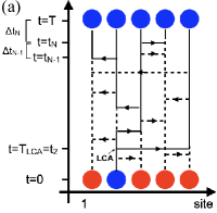
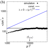
Figure 1: The genealogy and its implications. (a) Illustration of the history of mutation accumulation. Vertical lines represent mutational paths. Horizontal arrows mark loss/replacement events by which one cell copies its mutational configuration, in the direction of the arrow. Dashed lines are mutational paths that are lost, while bold lines are paths which survive until time $t=T$, constituting the genealogy. If $T$ is large enough, the genealogy possesses a single root, the last common ancestor (LCA). (b) Mean difference between maximum mutation number and the population mean, $\langle\Delta m^{*}\rangle=\langle m^{*}\rangle-\langle m_{i}\rangle$, as a function of $\mu T$, for fixed $N=10,000$, with $\lambda=\mu$. Points are results from Monte Carlo simulations; the dashed black line illustrates the saturation constant. The blue dashed line marks the scaling prediction for $\lambda=0$, $\langle\Delta m^{*}\rangle\sim(\mu T)^{1/2}$.

The tree structure of the genealogy is characterized by its branching times $t_{k}$, at which the branch number changes from $k-1$ to $k$ (see Fig. 1a), i.e. during the period $t_{k}<t<t_{k+1}$, the genealogy consists of $k$ branches. The branching times can be determined by following the genealogy backwards in time $\hat{t}=T-t$; a coalescent process Kingman (1982b); Hudson (1991); Wakely (2008). This results in branching times whose intervals $\Delta t_{k}:=t_{k+1}-t_{k}$ are exponentially distributed, with ${\rm Prob}(\Delta t_{k})=\langle\Delta t_{k}\rangle^{-1}e^{-\Delta t_{k}/\langle\Delta t_{k}\rangle}$ and mean branching times (see Supplemental Material)

$$\langle\Delta t_{k}\rangle=\frac{N}{k\,(k-1)}\frac{1}{\lambda}\,\,\,\,.$$ (5)

Importantly, the accumulation of mutations along a single branch follows a simple, independent Poisson process Hudson (1991) and thus the mean mutation number is simply $\langle m_{i}\rangle(T)=\mu T$.

For times $T$ large enough, if one follows the coalescent process far backwards in time $\hat{t}$, the number of branches reduces until $\hat{t}=\hat{T}_{LCA}:=T-t_{2}$, beyond which there is only a single one left, the last common ancestor (LCA) (see Fig. 1a). Thus, an LCA exists whenever $T>\hat{T}_{\rm LCA}$, which is on average $\langle\hat{T}_{\rm LCA}\rangle=\sum_{k=2}^{N}\langle\Delta t_{k}\rangle\approx N/\lambda$ (for $N\gg 1$). In that case, before the time $T_{\rm LCA}=T-\hat{T}_{\rm LCA}=t_{2}$, the genealogy corresponds to the mutational path of a single cell for which the maximum $m^{*}$ equals the mutation number $m$. Hence, it follows that $\Delta m^{*}=m^{*}-\langle m_{i}\rangle>0$ only for times larger than $T_{LCA}$, such that the statistics of $\Delta m^{*}$ does not explicitly depend on the total time $T$ if $T>\hat{T}_{\rm LCA}$. Indeed, Monte Carlo simulations of the model confirm this conjecture for $\langle\Delta m^{*}\rangle(T)$, as is illustrated in Fig. 1b for a high mutation rate $\mu=\lambda$, where a plateau is reached around $T\sim\langle\hat{T}_{\rm LCA}\rangle$. Note that this is in contrast to the case of purely asymmetric divisions, $\lambda=0$, for which $\langle\Delta m^{*}\rangle\sim(\mu T)^{1/2}$.

To support this finding for $T>\hat{T}_{\rm LCA}$ quantitatively, we note that the branching times are random and exponentially distributed. Thus, the branching of the genealogy corresponds to a Markov process, a branching process with initially two branches at time $T_{\rm LCA}$ with branching rate per branch $\nu_{k}:=1/\langle\Delta t_{k}\rangle k$. By approximating the random accumulation of mutations along each branch (Poisson process) by diffusive random walks in the variables $m_{i}-\mu T$ (valid for $\mu T\gg 1$), the mutation accumulation of the genealogy becomes an unbiased branching random walk (BRW). For unit branching rate, it has been shown Bramson (1978) that the CDF of the maximum $\Delta m^{*}$ of the BRW, $P^{*}_{N}(\Delta m_{c},\tau)={\rm Prob}(\Delta m^{*}(\tau)\leq\Delta m_{c})$, follows a Fisher-KPP-type equation Fisher (1937); Kolmogorov et al. (1937)

$$\partial_{\tau}P^{*}_{N}=D\,\frac{\partial^{2}P^{*}_{N}}{\partial\Delta m_{c}^{2}}-P^{*}_{N}[1-P^{*}_{N}]\,\,\,,$$ (6)

with the dimensionless time $\tau=\nu t$ measured in units of the constant branching time $\nu^{-1}$, and $D$, the diffusion constant of the random walk. The solution of this equation has the form

$$P^{*}_{N}(\Delta m_{c},\tau) =f(\Delta m_{c}-\tilde{m}(\tau))$$ (7)

with the median of $P^{*}_{N}$, $\tilde{m}(\tau)=2\sqrt{D}\,\tau+O(\ln\tau)$ Bramson (1978).

Here, the branching rate $\nu_{k}$ is not constant. By a step-wise rescaling of time in units of branching times as $\tau(t):=\nu_{k}(t-t_{k})+\tau_{k}$, with $\tau_{k}=\sum_{k^{\prime}=2}^{k-1}\nu_{k^{\prime}}\Delta t_{k^{\prime}}$ for the largest $t_{k}<t$, $k>2$, the corresponding BRW in the time scale $\tau$ has unit branching rate and effective diffusion constant $D_{k}:=\mu/2\nu_{k}$. While $D_{k}$ does not explicitly depend on time, we can take the ensemble average over the branch numbers $k$, $D(\tau):=\langle D_{k}\rangle_{k}|_{\tau}=\mu N/(2\lambda)\times\langle(k-1)^{-1}\rangle_{k}|_{\tau}$, to get an effective time-dependent diffusion constant. According to Ref. Fang and Zeitouni (2012) (see also Supplemental Material), for a diffusion constant $D(\tau^{\prime})$ that decreases over time $\tau^{\prime}<\tau=\tau(T)$, the CDF of the maximum of a BRW has the form of a Fisher-KPP wave, according to (7), but with

$$\tilde{m}(\tau) =\left[\int_{0}^{\tau}2\sqrt{D(\tau^{\prime})}\,d\tau^{\prime}\right](1-O(\tau^{-\frac{2}{3}}))\approx\mathcal{C}_{\tilde{m}}\sqrt{\frac{\mu N}{\lambda}}\,\,\,,$$ (8)

where $\mathcal{C}_{\tilde{m}}=\int_{0}^{\infty}\sqrt{2\langle(k-1)^{-1}\rangle_{k}|_{\tau^{\prime}}}\,d\tau^{\prime}$ is independent of the model parameters $N,T,\lambda$ and $\mu$. Here, we took the limit $\tau(T)\to\infty$, which is valid for large $N$, as this is a unit rate branching process with branch number $k(T)=N\approx e^{\tau}$. Thereby, terms of $O(\tau^{-\frac{2}{3}})$ are omitted, and the integral becomes independent of $N$. A numerical evaluation (see Supplemental Material) yields $\mathcal{C}_{\tilde{m}}\approx 1.79$.

As expected, $\tilde{m}$ becomes independent of $T$ if an LCA exists. The mean, $\langle\Delta m^{*}\rangle$, follows the same scaling in $N$ and $T$, since due to the wave property of the CDF it only differs by a constant. This confirms our previous conjecture and the simulation results for $\langle\Delta m^{*}\rangle(T)$ (Fig. 1b). In Fig. 2, we compare the theoretical results from Eq. (8) with results for $\langle\Delta m^{*}\rangle$ from Monte Carlo simulations, as a function of $N$. Here, $T$ was scaled with $N$ ($T=10\,N/\lambda$) to assure that $T>\hat{T}_{\rm LCA}$. The theory with fitted numerical constant $\mathcal{C}_{\tilde{m}}$ ($\mathcal{C}_{\tilde{m}}^{\rm fit}$, blue dashed line) shows excellent agreement with simulations, while the calculated value ($\mathcal{C}_{\tilde{m}}^{\rm th}=1.79$, red line) shows some deviation. These deviations are expected due to contributions with small $\tau^{\prime}$ in $\mathcal{C}_{\tilde{m}}$ (whose approximation is valid for large $\tau^{\prime}$). Remarkably, the predictions of the approximation are also valid for $\mu T\sim 1$ as shown in Fig. 2b for $\mu=0.001\,\lambda$.

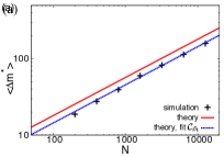
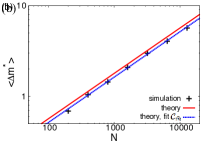
Figure 2: Mean maximum mutation number ahead of the mean, $\langle\Delta m^{*}\rangle$ as a function of $N$, for $T=10\,N/\lambda$ such that $T>\hat{T}_{\rm LCA}$. Shown are the results of Monte Carlo simulations (pluses), and theoretical predictions from the BRW approximation, Eq. (8), for fitted numerical constant $\mathcal{C}_{\tilde{m}}^{\rm fit}$ (blue dashed line) and theoretically estimated value (solid red line), $\mathcal{C}_{\tilde{m}}^{\rm th}=1.79$ for (a) $\mu=\lambda$ ($\mathcal{C}_{\tilde{m}}^{\rm fit}=1.43$) and (b) $\mu=0.001\lambda$ ($\mathcal{C}_{\tilde{m}}^{\rm fit}=1.63$) .

While the nonlinear form of the Fisher-KPP equation does not admit an exact solution, the CDF’s tail with $\bar{P}_{N}=1-P^{*}_{N}(\Delta m_{c},\tau)\ll 1$ can be mapped onto a simple diffusion equation with time-varying diffusion constant (see Supplemental Material). Since variances add linearly in this case, for $T>\hat{T}_{LCA}$ and $\Delta m_{c}\gg\tilde{m}$, the CDFs tail is that of a non-normalized Gaussian function,

$$P^{*}_{N}(\Delta m_{c})\sim 1-\frac{N\sigma_{\rm eff}\,e^{-\frac{\Delta m_{c}^{2}}{2\sigma_{\rm eff}^{2}}}}{\sqrt{2\pi}\,\Delta m_{c}}\,\,\,,$$ (9)

with

$$\sigma_{\rm eff}(\tau)=2\sqrt{\int_{0}^{\tau}D(\tau^{\prime})\,d\tau^{\prime}}\approx\mathcal{C}_{\sigma}\,\sqrt{\frac{\mu N}{\lambda}}\,\,\,,$$ (10)

where $\mathcal{C}_{\sigma}\approx\sqrt{\int_{0}^{\infty}2\langle(k-1)\rangle_{k}|_{\tau^{\prime}}\,d\tau^{\prime}}\approx 0.76$ (see Supplemental Material).

For $T<\hat{T}_{\rm LCA}$ the population may not possess an LCA. In this case the genealogy fragments into $k$ sub-genealogies $l=1,...,k$, each representing a subpopulation of $n_{l}$ cells, while $N=\sum_{l=1}^{k}n_{l}$. Each sub-genealogy, however, can again be approximated by a branching random walk, with a CDF $P_{l}(\Delta m_{c})$ having a Gaussian tail according to Eq. (9). Therefore, and since the subpopulations accumulate mutations independently from each other, the CDF of the whole population, $P^{*}_{N}(\Delta m_{c})$, is approximated for large $N$ by a Gumbel distribution according to Eq. (3) Bouchaud and Marc (1997), scaled by $\sigma_{\rm eff}$, and with effective number of independently distributed random variables, $k\approx N/\lambda T$ (see Supplemental Material). This CDF has then median and scaling width,

$$\tilde{m} \approx\mathcal{C}_{\sigma}\sqrt{2\,\ln\left(\frac{N}{\lambda T}\right)\mu T},\hskip 5.69054pt\sigma_{N}\approx\mathcal{C}_{\sigma}\sqrt{\frac{\mu T}{2\ln\left(\frac{N}{\lambda T}\right)}},$$ (11)

where $\mathcal{C}_{\sigma}$ is according to Eq. (10). The same scaling applies to $\langle\Delta m^{*}\rangle$.

Thus, we expect the scaling $\Delta m^{*}\sim\sqrt{\ln{N}}$, as for $\lambda=0$, but with a negative offset $-2\mathcal{C}_{\sigma}^{2}\ln(\lambda T)\mu T$ under the square root. Figure 3 shows Monte Carlo simulations of $\langle\Delta m^{*}\rangle$ together with the theory, with fitted $\mathcal{C}_{\sigma}^{\rm fit}$, which shows a good agreement in the shown range of $N$, for both large and small mutation rates, $\mu=\lambda$ and $\mu=0.001\lambda$. Deviations from the theoretically approximated value $\mathcal{C}_{\sigma}^{\rm th}=0.76$ are expected, for the same reasons as for $\mathcal{C}_{\tilde{m}}$ before, and furthermore for very large $N$, since the extreme value distribution of Poisson variables differs from the Gaussian approximation in this limit.

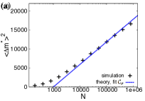
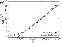
Figure 3: Squared mean maximum mutation number ahead of the population mean, $\langle\Delta m^{*}\rangle^{2}$ as a function of $N$, for fixed $T=1000/\lambda$. Shown are the results of Monte Carlo simulations (pluses) and the theory, Eq. (11), with fit parameter $\mathcal{C}_{\sigma}^{\rm fit}$ (dashed line) for (a) $\mu=\lambda$ ($\mathcal{C}_{\sigma}^{\rm fit}=1.13$) and (b) $\mu=0.001\lambda$ ($\mathcal{C}_{\sigma}^{\rm fit}=1.59$).

Finally, we consider the risk of accumulating a critical mutation number $m_{c}$, $\bar{P}_{N}(m_{c},T)=1-P_{N}^{*}(m_{c},T)$. In Figure 4, results from stochastic simulations for $\bar{P}_{N}(T)$ are shown for $m_{c}=6$ Armitage and Doll (1954); Tomlinson et al. (1996) with parameters chosen to match physiological conditions of human epidermal stem cells Martincorena et al. (2015); Simons (2016) (see figure caption), comparing a model of stochastic stem cell loss and replacement, $\lambda>0$, with the hypothetical case of asymmetric stem cell divisions, $\lambda=0$. As the front of $P^{*}_{N}(m_{c})$ moves with a speed $\mu+\partial_{t}\tilde{m}$, which is larger for $\lambda=0$ (see Figure 1b), it reaches the critical value $m_{c}=6$ earlier than for $\lambda>0$, resulting in an earlier increase of $\bar{P}_{N}(m_{c},T)$ in Figure 4a. Remarkably, the threshold of $m_{c}=6$ mutations is already frequently exceeded for mean mutation numbers $\mu T<1$, which demonstrates that the acquisition of a critical number of mutations is indeed dominated by extreme values. In Figure 4b, the risk ratio between the risk $\bar{P}_{N}|_{\lambda=0}$ for asymmetric divisions and that for symmetric divisions, $\bar{P}_{N}|_{\lambda>0}$, is shown. One observes a non-monotonic behavior: for intermediate times the ratio is large, while it approaches one for large times. The initial growth of the ratio is due to the smaller slope in the tail for $\lambda>0$, $1/\sigma^{\lambda>0}_{N}\sim\sqrt{\ln(N/(\lambda T))}$ compared to the slope $1/\sigma^{\lambda=0}_{N}\sim\sqrt{\ln(N)}$ for $\lambda=0$. Once $\bar{P}_{N}|_{\lambda=0}$ has saturated, however, $\bar{P}_{N}|_{\lambda>0}$ catches up with the latter until both approach $\bar{P}_{N}=1$. This provides a theoretical foundation for claims that the risk of tumor initiation is decreased by stochastic stem cell loss and replacement Shahriyari and Komarova (2013); McHale and Lander (2014), yet this advantage is limited to intermediate time scales.

Until now, we have considered an “infinite-dimensional” process in which any cell may replace another. However, the majority of biological tissues are low-dimensional, where stem cell loss and replacement occur between neighboring cells in tubular (one-dimensional), epithelial (two-dimensional) or volumnar (three-dimensional) settings. Such situations can be modeled by embedding cells on a $d$-dimensional regular lattice, allowing replacement only between neighboring cells Klein et al. (2008); Klein and Simons (2011). In this case, our general theory remains valid, based on the mapping of the genealogy on a BRW; only the distribution of branching times, $\Delta t_{k}$, differs (see Supplemental Material). Nonetheless, only for $d=1$ and $T>\hat{T}_{\rm LCA}$, a significantly different scaling with $\tilde{m}\sim N\sqrt{\mu/\lambda}$ is observed, compared to the infinite-dimensional case.

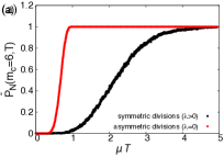
Figure 4: Probability $\bar{P}_{N}(T)$ of accumulating a critical number of $m_{c}=6$ mutations in an area of 0.1 ${\rm cm}^{2}$, corresponding to $10^{5}$ cells. (a) $\bar{P}_{N}$ as function of time for physiological parameters of human eyelid Martincorena et al. (2015); Simons (2016), with $\mu=0.27/(63\,\mbox{years})$ and $\lambda=0.5/\mbox{week}$, corresponding to $\lambda\approx 6000\mu$ (black points), and for the hypothetical case $\lambda=0$ (red points). (b) The risk ratio $(\bar{P}_{N})^{\lambda=0}/(\bar{P}_{N})^{\lambda>0}$ for the two scenarios from (a).

In summary, we have studied the asymptotic behavior, with time $T$ and cell number $N$, of the maximum mutation number statistics in a renewing cell population, in which cells may be stochastically lost and replaced (Moran process). This is of importance if multiple neutral or near-neutral mutations can cooperate through epistasis to trigger hyper-proliferation, a potential tumor initiating event. We showed that, for a non-zero cell replacement rate, $\lambda>0$, the difference between the average maximum mutation number and the population mean, $\langle\Delta m^{*}\rangle$, saturates to a constant value when scaled with $T$. Using an analogy to branching random walks, we showed that the value of this constant scales as $(\mu N/\lambda)^{1/2}$ for $\lambda>0$, while in the absence of symmetric loss/replacement, $\lambda=0$ (e.g. for asymmetric stem cell divisions only), $\langle\Delta m^{*}\rangle$ scales with time and cell number as $(\mu T\ln(N))^{1/2}$. If $T$ is fixed, $\langle\Delta m^{*}\rangle$ scales as $(\mu T\ln(N/(\lambda T)))^{1/2}$ for $\lambda>0$ and large $N\gg\lambda T$. From this result, it follows that at intermediate time scales, the risk of triggering hyper-proliferation is higher for asymmetric than for symmetric stem cell divisions, yet these probabilities converge for large times. Crucially, our theory also applies in a low-dimensional setting, where cell loss and replacement occurs between neighbors, albeit with a different scaling dependence for one-dimensional structures.

We thank Steffen Rulands for valuable discussions and for help with literature research on genealogies and the coalescent process. We further are thankful for the support by a EPSRC Critical Mass Grant and a DFG Research Fellowship.

References

- Knudson (1971) A. G. Knudson, Proc. Natl. Acad. Sci. 68, 820 (1971).
- Ashworth et al. (2011) A. Ashworth, C. J. Lord, and J. S. Reis-Filho, Cell 145, 30 (2011).
- Hartman et al. (2001) J. L. Hartman, B. Garvik, and L. Hartwell, Science 291, 1001 (2001).
- de Visser et al. (2003) J. A. G. M. de Visser, et al., Evolution 57, 1959 (2003).
- Gu et al. (2003) Z. Gu, et al., Nature 421, 63 (2003).
- Simons (2016) B. D. Simons, Proc. Natl. Acad. Sci. 113, 128 (2016).
- Martincorena et al. (2015) I. Martincorena, et al., Science 348, 880 (2015).
- Moore (2005) J. H. Moore, Nature Genetics 37, 13 (2005).
- Jasnos and Korona (2007) L. Jasnos and R. Korona, Nature Genetics 39, 550 (2007).
- Komarova (2014) N. L. Komarova, Proc. Natl. Acad. Sci. 111, 10789 (2014).
- Wagstaff et al. (2013) L. Wagstaff, G. Kolahgar, and E. Piddini, Trends in Cell Biology 23, 160 (2013).
- Alcolea et al. (2014) M. P. Alcolea, et al., Nature Cell Biology 16, 615 (2014).
- Brown et al. (2017) S. Brown, et al., Nature (2017).
- Cooper (2000) G. M. Cooper, in The Cell: A Molecular Approach. 2nd edition. (Sinauer Associates;, 2000).
- Alonso and Fuchs (2003) L. Alonso and E. Fuchs, Proc. Natl. Acad. Sci. 100, 11830 (2003).
- Barker et al. (2007) N. Barker, et al., Nature 449, 1003 (2007).
- Potten (1974) C. S. Potten, Cell Tissue Kinet. 7, 77 (1974).
- Clayton et al. (2007) E. Clayton, et al., Nature 446, 185 (2007).
- Lopez-Garcia et al. (2010) C. Lopez-Garcia, A. M. Klein, B. D. Simons, and D. J. Winton, Science 330, 822 (2010).
- Armitage and Doll (1954) P. Armitage and R. Doll, British Journal of Cancer 8, 1 (1954).
- Armitage and Doll (1957) P. Armitage and R. Doll, British Journal of Cancer 11, 161 (1957), eprint 209.
- Portier et al. (1996) C. J. Portier, A. Kopp-Schneider, and C. D. Sherman, Mathematical Biosciences 135, 129 (1996).
- Bozic et al. (2010) I. Bozic, et al., Proc. Natl. Acad. Sci. 107, 18545 (2010).
- McHale and Lander (2014) P. T. McHale and A. D. Lander, PLoS computational biology 10, e1003802 (2014).
- Shahriyari and Komarova (2013) L. Shahriyari and N. L. Komarova, PLoS ONE 8, e76195 (2013).
- Moran (1958) P. A. P. Moran, Mathematical Proceedings of the Cambridge Philosophical Society 54, 60 (1958).
- Leadbetter et al. (1983) M. R. Leadbetter, G. Lindgren, and H. Rootzén, Extremes and related properties of random sequences and processes (Springer, New York, 1983).
- Bouchaud and Marc (1997) J.-P. Bouchaud and M. Marc, J. Phys. A: Math. Gen. 30, 7997 (1997).
- Kingman (1982a) J. Kingman, Journal of Applied Probability 19, 27 (1982a).
- Hudson (1991) R. R. Hudson, in Oxford Surveys in Evolutionary Biology, edited by D. Futuyama and J. Antonovics (1991), p. 1, 7th ed.
- Kingman (1982b) J. Kingman, Stochastic Processes and their Applications 13, 235 (1982b).
- Wakely (2008) J. Wakely, in Coalescent Theory: An Introduction (W. H. Freeman, 2008).
- Bramson (1978) M. D. Bramson, Communications on Pure and Applied Mathematics 31, 531 (1978).
- Fisher (1937) R. A. Fisher, Annals of Eugenics 7, 355 (1937).
- Kolmogorov et al. (1937) A. Kolmogorov, I. Petrovskii, and N. Piscunov, Byul. Moskovskogo Gos. Univ. 1, 1 (1937).
- Fang and Zeitouni (2012) M. Fang and O. Zeitouni, J. Stat. Phys. 149, 1 (2012).
- Tomlinson et al. (1996) I. P. M. Tomlinson, M. R. Novelli, and W. F. Bodmer, Proc. Natl. Acad. Sci. 93, 14800 (1996).
- Klein et al. (2008) A. M. Klein, D. P. Doupé, P. H. Jones, and B. D. Simons, Phys. Rev. E 77, 031907 (2008).
- Klein and Simons (2011) A. M. Klein and B. D. Simons, Development 138, 3103 (2011).