Learning Task Specifications from Demonstrations
Abstract
Real-world applications often naturally decompose into several sub-tasks. In many settings (e.g., robotics) demonstrations provide a natural way to specify the sub-tasks. However, most methods for learning from demonstrations either do not provide guarantees that the artifacts learned for the sub-tasks can be safely recombined or limit the types of composition available. Motivated by this deficit, we consider the problem of inferring Boolean non-Markovian rewards (also known as logical trace properties or specifications) from demonstrations provided by an agent operating in an uncertain, stochastic environment. Crucially, specifications admit well-defined composition rules that are typically easy to interpret. In this paper, we formulate the specification inference task as a maximum a posteriori (MAP) probability inference problem, apply the principle of maximum entropy to derive an analytic demonstration likelihood model and give an efficient approach to search for the most likely specification in a large candidate pool of specifications. In our experiments, we demonstrate how learning specifications can help avoid common problems that often arise due to ad-hoc reward composition.
1 Introduction
In many settings (e.g., robotics) demonstrations provide a natural way
to specify a task. For example, an agent (e.g., human expert) gives
one or more demonstrations of the task from which we seek to
automatically synthesize a policy for the robot to execute.
Typically, one models the demonstrator as episodically operating
within a dynamical system whose transition relation only depends on
the current state and action (called the Markov
condition). However, even if the dynamics are Markovian, many
problems are naturally modeled in non-Markovian terms (see
Ex 1).
Example 1.
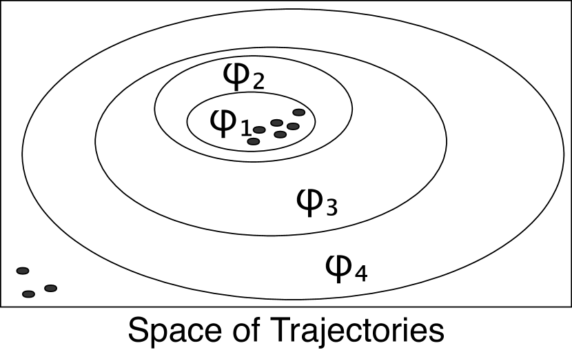
Consider the task illustrated in Figure 1. In
this task, the agent moves in a discrete gridworld and can take
actions to move in the cardinal directions (north, south, east,
west). Further, the agent can sense abstract features of the
domain represented as colors. The task is to reach any of the
yellow (recharge) tiles without touching a red tile (lava) – we
refer to this sub-task as YR. Additionally, if a blue tile
(water) is stepped on, the agent must step on a brown tile
(drying tile) before going to a yellow tile – we refer to this
sub-task as BBY. The last constraint requires recall of two
state bits of history (and is thus not Markovian): one bit for whether
the robot is wet and another bit encoding if the robot recharged
while wet.
![[Uncaptioned image]](/html/1710.03875/assets/imgs/simple_gridworld_doshow.png) Figure 1:
Figure 1:
Further, like Ex 1, many tasks are naturally decomposed into several sub-tasks. This work aims to address the question of how to systematically and separately learn non-Markovian sub-tasks such that they can be readily and safely recomposed into the larger meta-task.
Here, we argue that non-Markovian Boolean specifications provide a powerful, flexible, and easily transferable formalism for task representations when learning from demonstrations. This stands in contrast to the quantitative scalar reward functions commonly associated with Markov Decision Processes. Focusing on Boolean specifications has certain benefits: (1) The ability to naturally express tasks with temporal dependencies; (2) the ability to take advantage of the compositionality present in many problems, and (3) use of formal methods for planning and verification [29].
Although standard quantitative scalar reward functions could be used to learn this task from demonstrations, three issues arise. First, consider the problem of temporal specifications: reward functions are typically Markovian, so requirements like those in Ex 1 cannot be directly expressed in the task representation. One could explicitly encode time into a state and reduce the problem to learning a Markovian reward on new time-dependent dynamics; however, in general, such a reduction suffers from an exponential blow up in the state size (commonly known as the curse of history [24]). When inferring tasks from demonstrations, where different hypotheses may have different historical dependencies, naïvely encoding the entire history quickly becomes intractable.
A second limitation relates to the compositionality of task representations. As suggested, Ex 1 naturally decomposes into two sub-tasks. Ideally, we would want an algorithm that could learn each sub-task and combine them into the complete task, rather than only be able to learn single monolithic tasks. However, for many classes of quantitative rewards, "combining" rewards remains an ad-hoc procedure. The situation is further exacerbated by humans being notoriously bad at anticipating or identifying when quantitative rewards will lead to unintended consequences [11], which poses a serious problem for AI safety [1] and has led to investigations into reward repair [9]. For instance, we could take a linear combination of rewards for each of the subtasks in Ex 1, but depending on the relative scales of the rewards, and temporal discount rate, wildly different behaviors would result.
In fact, the third limitation - brittleness due to simple changes in the environment - illustrates that often, the correctness of the agent can change due to a simple change in the environment. Namely, imagine for a moment we remove the water and drying tiles from Fig 1 and attempt to learn a reward that encodes the “recharge while avoid lava” task in Ex 1. Fig 2(a) illustrates the reward resulting from performing Maximum Entropy Inverse Reinforcement Learning [35] with the demonstrations shown in Fig 1 and the binary features: red (lava tile), yellow (recharge tile), and “is wet”. As is easy to verify, a reward optimizing agent, , with a discount factor of would generate the trajectory shown in Fig 2(a) which avoids lava and eventually recharges.
Unfortunately, using the same reward and discount factor on a nearly identical world can result in the agent entering the lava. For example, Fig 2(b) illustrates the learned reward being applied to a change in the gridworld where the top left charging tile has been removed. An acceptable trajectory is indicated via a dashed arrow. Observe that now the discounted sum of rewards is maximized on the solid arrow’s path, resulting in the agent entering the lava! While it is possible to find new discount factors to avoid this behavior, such a supervised process would go against the spirit of automatically learning the task.
Finally, we briefly remark that while non-Markovian Boolean rewards cannot encode all possible rewards, e.g., “run as fast as possible”, often times such objectives can be reframed as policies for a Boolean task. For example, consider modeling a race. If at each time step there is a non-zero probability of entering a losing state, the agent will run forward as fast as possible even for the Boolean task “win the race”.
Thus, quantitative Markovian rewards are limited as a task representation when learning tasks containing temporal specifications or compositionality from demonstrations. Moreover, the need to fine tune learned tasks with such properties seemingly undercuts the original purpose of learning task representations that are generalizable and invariant to irrelevant aspects of a task [21].
Related Work: Our work is intimately related to Maximum Entropy Inverse Reinforcement Learning. In Inverse Reinforcement Learning (IRL) [23] the demonstrator, operating in a stochastic environment, is assumed to attempt to (approximately) optimize some unknown reward function over the trajectories. In particular, one traditionally assumes a trajectory’s reward is the sum of state rewards of the trajectory. This formalism offers a succinct mechanism to encode and generalize the goals of the demonstrator to new and unseen environments.
In the IRL framework, the problem of learning from demonstrations can then be cast as a Bayesian inference problem [26] to predict the most probable reward function. To make this inference procedure well-defined and robust to demonstration/modeling noise, Maximum Entropy IRL [35] appeals to the principle of maximum entropy [12]. This results in a likelihood over the demonstrations which is no more committed to any particular behavior than what is required for matching the empirically observed reward expectation. While this approach was initially limited to learning a linear combination of feature vectors, IRL has been successfully adapted to arbitrary function approximators such as Gaussian processes [19] and neural networks [8]. As stated in the introduction, while powerful, traditional IRL provides no principled mechanism for composing the resulting rewards.
To address this deficit, composition using soft optimality has recently received a fair amount of attention; however, the compositions are limited to either strict disjunction (do X or Y) [30] [31] or conjunction (do X and Y) [10]. Further, because soft optimality only bounds the deviation from simultaneously optimizing both rewards, optimizing the composition does not preclude violating safety constraints embedded in the rewards (e.g., do not enter the lava).
The closest work to ours is recent work on inferring Linear Temporal Logic (LTL) by finding the specification that minimizes the expected number of violations by an optimal agent compared to the expected number of violations by an agent applying actions uniformly at random [16]. The computation of the optimal agent’s expected violations is done via dynamic programming on the explicit product of the deterministic Rabin automaton [7] of the specification and the state dynamics. A fundamental drawback to this procedure is that due to the curse of history, it incurs a heavy run-time cost, even on simple two state and two action Markov Decision Processes. We also note that the literature on learning logical specifications from examples (e.g., [15, 33, 20]), does not handle noise in examples while our approach does. Finally, once a specification has been identified, one can leverage the rich literature on planning using temporal logic to synthesize a policy [17, 28, 27, 13, 14].
Contributions: (i) We formulate the problem of learning specifications from demonstrations in terms of Maximum a Posteriori inference. (ii) To make this inference well defined, we appeal to the principle of maximum entropy culminating in the distribution given (17). The main contribution of this model is that it only depends on the probability the demonstrator will successfully perform task and the probability that the task is satisfied by performing actions uniformly at random. Because these properties can be estimated without explicitly unrolling the dynamics in time, this model avoids many of the pitfalls characteristic to the curse of history. (iii) We provide an algorithm that exploits the piece-wise convex structure in our posterior model (17) to efficiently perform Maximum a Posteriori inference for the most probable specification.
Outline: In Sec 2, we define specifications and probabilistic automata (Markov Decision Processes without rewards). In Sec 3, we introduce the problem of specification inference from demonstrations, and inspired by Maximum Entropy IRL [35], develop a model of the posterior probability of a specification given a sequence of demonstrations. In Sec 4, we develop an algorithm to perform inference under (17). Finally, in Sec 5, we demonstrate how due to their inherent composability, learning specifications can avoid common bugs that often occur due to ad-hoc reward composition.
2 Background
We seek to learn specifications from demonstrations provided by a teacher who executes a sequence of actions that probabilistically changes the system state. For simplicity, we assume that the set of actions and states are finite and fully observed. The system is naturally modeled as a probabilistic automaton111Probabilistic Automata are often constructed as a Markov Decision Process, , without its Markovian reward map , denoted . formally defined below: {mddef}[Probabilistic Automaton] A probabilistic automaton is a tuple , where is the finite set of states, is the initial state, is the finite set of actions, and specifies the transition probability of going from to given action , i.e. and for all states .
[Trace] A sequence of state/action pairs is called a trace (trajectory, demonstration). A trace of length is an element of . Next, we develop machinery to distinguish between desirable and undesirable traces. For simplicity, we focus on finite trace properties, referred to as specifications, that are decidable within some fixed time steps, e.g., “event A occurred in the last 20 steps”. {mddef}[Specification] Given a set of states , a set of actions , and a fixed trace length , a specification is a subset of traces . We define , , and . A collection of specifications, , is called a concept class. Finally, we abuse notation and use to also denote its indicator function (interpreted as a non-Markovian Boolean reward),
| (1) |
Specifications may be given in formal notation, as sets or automata. Further, each representation facilitates defining a plethora of composition rules. For example, consider two specifications, , that encode tasks and respectively and the composition rule . Because the agent only receives a non-zero reward if , a reward maximizing agent must necessarily perform tasks and simultaneously. Thus, corresponds to conjunction (logical and). Similarly, maximizing corresponds to disjunction (logical or). One can also encode conditional requirements using subset inclusion, e.g., maximizing corresponds to task A triggering task B.
Complicated temporal connectives can also be defined using temporal logics [25] or automata [32]. For our purposes, it suffices to informally extend propositional logic with three temporal operators: (1) Let , read “historically ”, denote that property held at all previous time steps. (2) Let , read “once ”, denote that the property at least once held in the past. (3) Let , read “ since ”, denote that the property that has held every time step after last held. The true power of temporal operators is realized when they are composed to make more complicated sentences. For example, translates to “it was always the case that if was true, then has held since the last time held.”. Observe that the property BBY from the introductory example takes this form, , i.e., “Historically, if the agent had once visited blue and is currently visiting yellow, then the agent has not visited blue since it last visited brown”.
3 Specification Inference from Demonstrations
In the spirit of Inverse Reinforcement Learning, we now seek to find the specification that best explains the behavior of the agent. We refer to this as Specification Inference from Demonstrations. {mddef}[Specification Inference from Demonstrations] The specification inference from demonstrations problem is a tuple where is a probabilistic automaton, is a (multi-)set of -length traces drawn from an unknown distribution induced by a teacher attempting to demonstrate some unknown specification within , and a concept class of specifications.
A solution to is:
| (2) |
where denotes the probability that the teacher demonstrated given the observed traces, , and the dynamics, . To make this inference well-defined, we make a series of assumptions culminating in (17).
Likelihood of a demonstration: We begin by leveraging the principle of maximum entropy to disambiguate the likelihood distributions. Concretely, define:
| (3) |
where and are the projected sequences of states and actions of respectively, to be the weight of each possible demonstration induced by dynamics . Given a demonstrator who on average satisfies the specification with probability , we approximate the likelihood function by:
| (4) |
where , are normalization factors such that and . For a detailed derivation that (4) is the maximal entropy distribution, we point the reader to [18]. Next observe that due to the Boolean nature of , (4) admits a simple closed form:
| (5) |
where in general we use to denote the probability of satisfying a specification using uniformly random actions. Thus, we denote by the probability of randomly generating demonstration within . Further, note that by the law of the excluded middle, for any specification: .
Proof Sketch.
Likelihood of a set of demonstrations: If the teacher gives a finite sequence of length demonstrations, , drawn i.i.d. from (5), then the log likelihood, , of under (5) is:222 We have suppressed a multinomial coefficient required if any two demonstrations are the same. However, this term will not change as varies, and thus cancels when comparing across specifications.
| (7) |
where by definition we take and .
Next, observe that is the information gain (KL divergence) between two Bernoulli distributions with means and resp. Syntactically, let denote a Bernoulli distribution with mean and denote the information gain when using distribution compared to . If is “representative” such that , we can (up to a independent normalization) approximate (7):
| (8) |
Where denotes approximately proportional to. Unfortunately, the approximation implies that, which introduces the undesirable symmetry, , into (8). To break this symmetry, we assert that the demonstrator must be at least as good as random. Operationally, we assert that and is otherwise uniform. Finally, we arrive at the posterior distribution given in (17), where denotes an indicator function.
| (17) |
4 Algorithm
In this section, we exploit the structure imposed by (17) to efficiently search for the most probable specification (2) within a (potentially large) concept class, . Namely, observe that under (17), the specification inference problem (2) reduces to maximizing the information gain over random actions.
| (18) |
Because gradients on
and are not well-defined,
gradient descent based algorithms are not applicable. Further, while
evaluating if a trace satisfies a specification is fairly efficient
(and thus our approximation to is assumed easy to compute), computing
is in general known to be
-complete [2].
Nevertheless, in practice, moderately efficient methods
for computing or approximating exist including
Monte Carlo simulation [22] and weighted model
counting [5] via Binary Decision
Diagrams (BDDs) [3] or repeated SAT
queries [4]. As such, we seek an
algorithm that poses few queries. We begin
with the observation that adding a trace to a
specification cannot lower its probability of satisfaction under random actions.
Lemma 1.
implies
and
.
Proof.
The probability of sampling an element of a
set monotonically increases as elements are added to the set
independent of the fixed underlying distribution over elements.
∎
Further, note that (and thus, our approximation to ) can only take on possible values. This suggests a piece-wise analysis of (18) by conditioning on the value of . {mddef} Given candidate specifications and a subset of demonstrations define,
| (19) |
The next key observation is that monotonically decreases in .
Lemma 2.
Proof.
To begin, observe that is always
non-negative. Due to the
indicator,
for all . Next, observe that
is convex due to the convexity of the on Bernoulli
distributions and is minimized at (KL Divergence
of identical distributions is ). Thus, monotonically
decreases as increases.
∎
These insights are then combined in Theorem 1
and illustrated in Fig 3.
Theorem 1.
If denotes a sequence of specifications,
, ordered by subset
inclusion and is an arbitrary subset of demonstrations, then:
(20)
Proof.
is monotonically increasing on
(Lemma 1). Via Lemma 2
is monotonically decreasing and thus the maximum of
must occur at the beginning of
.
∎
Lattice Concept Classes.
Theorem 1 suggests specializing to concept classes where determining subset relations is easy. We propose studying concept classes organized into a finite (bounded) lattice, (), that respects subset inclusion: . To enforce the bounded constraint, we assert that and are always assumed to be in and act as the bottom and top of the partial order respectively. Intuitively, this lattice structure encodes our partial knowledge of which specifications imply other specifications. These implication relations can be represented as a directed graph where the nodes correspond to elements of and an edge is present if the source is known to imply the target. Because implication is transitive, many of the edges can be omitted without losing any information. The graph resulting from this transitive reduction is called a Hasse diagram [6] (See Fig 4). In terms of the graphical model, the Hasse diagram encodes that for certain pairs of specifications, , we know that or .
Inference on chain concept classes.
Sequences of specifications ordered by subset inclusion generalize
naturally to ascending chains.
Definition 1 (Chains and Anti-Chains).
Given a partial order , an ascending chain (or just
chain) is a sequence of elements of ordered by . The smallest element of the chain is denoted, . Finally,
an anti-chain is a set of incomparable elements. An anti-chain
is called maximal if no element can be added to it without
making two of its elements comparable.
Recasting Theorem 1 in the parlance of chains yields:
Corollary 1.
If is a subset of demonstrations and
is a chain in then:
(21)
Observe that if the lattice, is itself a chain, then there are at most non-empty demonstration partitions, . In fact, the non-empty partitions can be re-indexed by the cardinality of , e.g., . Further, note that since chains are totally ordered, the smallest element of each non-empty partition can be found by performing a binary search (indicated by find_smallest below). These insights are combined into Algorithm 1 with a relativized run-time analysis given in Thm 2.
Theorem 2.
Let and respectively represent the worst case execution time of computing and for in chain . Given demonstrations , Alg 1 runs in time: (22)Proof Sketch.
A binary search over elements takes time. There are binary searches required to find the smallest element of each partition. Finally, for each smallest element, a single random satisfaction query is made. ∎Lattice inference. Of course, in general, is not a chain, but a complicated lattice. Nevertheless, observe that any path from to is a chain. Further, the smallest element of each partition must either be the same specification or incomparable in . That is, for each , the set:
| (23) |
is a maximal anti-chain. Thus,
Corollary 1 can be extended to:
Corollary 2.
Given a lattice and demonstrations :
(24)
Recalling that increases on paths from to ,
we arrive at the following simple algorithm which takes as input the
demonstrations and the lattice encoded as a directed acyclic graph
rooted at . (i) Perform a breadth first traversal (BFT) of the
lattice starting at (ii) During
the traversal, if specification has a larger than
all of its direct predecessors, then check if it is more probable
than the best specification seen so far (if so, make it the most probable
specification seen so far). (iii) At the end of the traversal, return
the most probable specification. Pseudo code is provided in
Algorithm 2 with a run-time analysis given in Theorem 3.
Theorem 3.
Let be a bounded partial order encoded as a Directed Acyclic Graph (DAG), , with vertices and edges . Further, let denote the largest anti-chain in . If and respectively represent the worst case execution time of computing and , then for demonstrations , Alg 2 runs in time: (25)Proof sketch.
BFT takes . Further, for each node, is computed (). Finally, for each node in each of the candidate anti-chains , is computed. Since is the size of the largest anti-chain, this query happens no more than times. ∎5 Experiments and Discussion
Scenario. Recall our introductory gridworld example Ex 1. Now imagine that the robot is pre-programmed to perform task the “recharge and avoid lava” task, but is unaware of the second requirement, “do not recharge when wet”. To signal this additional constraint to the robot, the human operator provides the five demonstrations shown in Fig 1. We now illustrate how learning specifications rather than Markovian rewards enables the robot to safely compose the new constraint with its existing knowledge to perform the joint task in a manner that is robust to changes in the task.
To begin, we assume the robot has access to the Boolean features: red (lava tile), blue (water tile), brown (drying tile), and yellow (recharge tile). Using these features, the robot has encoded the “recharge and avoid lava” task as: .
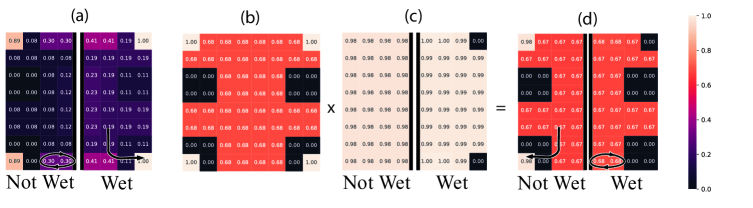 Figure 5:
Learned rewards on the task discussed in Ex 1.
(a) Rewards for the task YR and BBY. Arrows indicate how agents who are trying to maximize reward would behave (left is a myopic agent; right is non-myopic agent).
(b) Rewards for the sub-task YR.
(c) Rewards for the sub-task BBY.
(d) Rewards when YR and BBY are combined multiplicatively.
(a)-(c) Used MaxEnt IRL to infer rewards. In (a), (c), and (d) because
the gridworld is symmetric, we use the left (resp. right) side to show the
case where the robot is not wet (wet). Colors indicate magnitude of reward at that
location, where lighter indicates higher reward.
MaxEnt: We began by applying MaxEnt on all of the features to
learn the monolithic task. The resulting reward structure is shown in
Fig 5a. However, as Fig 5a illustrates, a
myopic agent is not incentivized to make progress towards the
recharging stations and a non-myopic agent will enter the lava to
reach the recharge station at the bottom. Next, we retrained on
subsets of the features to learn the sub-tasks (see Fig 5b
and Fig 5c). Observe that while the two reward
structures encode YR and BBY individually, it is not obvious how to
compose the rewards to jointly encode YR and BBY. For example,
just averaging makes the agent no longer avoid the lava. Taking the
minimum means that if the agent becomes wet it loses its incentive to
dry off or visit the yellow. Multiplication almost works, but suffers
from similar bugs as the monolithically learned reward (see Fig 5d).
Figure 5:
Learned rewards on the task discussed in Ex 1.
(a) Rewards for the task YR and BBY. Arrows indicate how agents who are trying to maximize reward would behave (left is a myopic agent; right is non-myopic agent).
(b) Rewards for the sub-task YR.
(c) Rewards for the sub-task BBY.
(d) Rewards when YR and BBY are combined multiplicatively.
(a)-(c) Used MaxEnt IRL to infer rewards. In (a), (c), and (d) because
the gridworld is symmetric, we use the left (resp. right) side to show the
case where the robot is not wet (wet). Colors indicate magnitude of reward at that
location, where lighter indicates higher reward.
MaxEnt: We began by applying MaxEnt on all of the features to
learn the monolithic task. The resulting reward structure is shown in
Fig 5a. However, as Fig 5a illustrates, a
myopic agent is not incentivized to make progress towards the
recharging stations and a non-myopic agent will enter the lava to
reach the recharge station at the bottom. Next, we retrained on
subsets of the features to learn the sub-tasks (see Fig 5b
and Fig 5c). Observe that while the two reward
structures encode YR and BBY individually, it is not obvious how to
compose the rewards to jointly encode YR and BBY. For example,
just averaging makes the agent no longer avoid the lava. Taking the
minimum means that if the agent becomes wet it loses its incentive to
dry off or visit the yellow. Multiplication almost works, but suffers
from similar bugs as the monolithically learned reward (see Fig 5d).
Concept Class. We designed the robot’s concept class to be the conjunction of the known requirements and a specification generated by the grammar on the right. The motivation in choosing this grammar was that (i) it generates a moderately large concept class (930 possible specifications after pruning trivially false specifications), and (ii) it contains several interesting alternative tasks such as , which semantically translates to: “the robot should be wet before entering lava”. To generate
Concept Class Grammar: {bnf*} \bnfprod \bnfpnH\bnfsp \bnfor\bnfpnP\bnfsp\bnfprod \bnfpn \bnfor\bnfpn \bnfts \bnfpn\bnfprod \bnfpn \bnfor\bnfpn \bnfsp\bnfts\bnfsp\bnfpn \bnfor\bnfpn \bnfsp\bnftsS\bnfsp\bnfpn\bnfprod \bnftdAP \bnfor¬\bnftdAP\bnfprod AP \bnftdyellow \bnfor\bnftdred \bnfor\bnftdbrown \bnfor\bnftdblue
the edges in Hasse diagram, we unrolled the formula into their corresponding Boolean formula and used a SAT solver to determine subset relations. While potentially slow, we make three observations regarding this process: (i) the process was trivially parallelizable (ii) so long as the atomic predicates remain the same, this Hasse diagram need not be recomputed since it is otherwise invariant to the dynamics (iii) most of the edges in the resulting diagram could have been syntactically identified using well known identities on temporal logic formula.
Computing . To perform random satisfaction rate queries, , we first ran Monte Carlo to get a coarse estimate and we symbolically encoded the dynamics, color sensor, and specification into a Binary Decision Diagram to get exact values. This data structure serves as an incredibly succinct encoding of the specification aware unrolling of the dynamics, which in practice avoids the exponential blow up suggested by the curse of history. We then counted the number of satisfying assignments and divided by the total possible number of satisfying assignments.333One can add probabilities to transitions by adding to transition constraints additional fresh variables such that the number of satisfying assignments is proportional to the probability. On average in these candidate pools, each query took seconds with a standard deviation of seconds.
Results. Running a fairly unoptimized implementation of Algorithm 2 on the concept class and demonstrations took approximately 95 seconds and resulted in 172 queries ( of the concept class). The inferred additional requirement was which exactly captures the do not recharge while wet constraint. Compared to a brute force search over the concept class, our algorithm offered an approximately 5.5 fold improvement. Crucially, there exists controllable trajectories satisfying the joint specification:
| (26) |
Thus, a specification optimizing agent must jointly perform both tasks. This holds true even under task changes such as that in Fig 2. Further, observe that it was fairly painless to incorporate the previously known recharge while avoiding lava constraints. Thus, in contrast to quantitative Markovian rewards, learning Boolean specifications enabled encoding compositional temporal specifications that are robust to changes in the environment.
6 Conclusion and Future work
Motivated by the problem of compositionally learning from demonstrations, we developed a technique for learning binary non-Markovian rewards, which we referred to as specifications. Because of their limited structure, specifications enabled first learning sub-specifications for subtasks and then later creating a composite specifications that encodes the larger task. To learn these specifications from demonstrations, we applied the principle of maximum entropy to derive a novel model for the likelihood of a specification given the demonstrations. We then developed an algorithm to efficiently search for the most probable specification in a candidate pool of specifications in which some subset relations between specifications are known. Finally, in our experiment, we gave a concrete instance where using traditional learning composite reward functions is non-obvious and error-prone, but inferring specifications enables trivial composition. Future work includes extending the formalism to infinite horizon specifications, continuous dynamics, characterizing the optimal set of teacher demonstrations under our posterior model [34], efficiently marginalizing over the whole concept class and exploring alternative data driven methods for generating concept classes.
Acknowledgments. We would like to thank the anonymous referees as well as Daniel Fremont, Markus Rabe, Ben Caulfield, Marissa Ramirez Zweiger, Shromona Ghosh, Gil Lederman, Tommaso Dreossi, Anca Dragan, and Natarajan Shankar for their useful suggestions and feedback. The work of the authors on this paper was funded in part by the US National Science Foundation (NSF) under award numbers CNS-1750009, CNS-1740079, CNS-1545126 (VeHICaL), the DARPA BRASS program under agreement number FA8750–16–C0043, the DARPA Assured Autonomy program, by Toyota under the iCyPhy center and the US ARL Cooperative Agreement W911NF-17-2-0196.
References
- [1] D. Amodei, C. Olah, J. Steinhardt, P. Christiano, J. Schulman, and D. Mané. Concrete problems in AI safety. arXiv preprint arXiv:1606.06565, 2016.
- [2] F. Bacchus, S. Dalmao, and T. Pitassi. Algorithms and complexity results for #SAT and Bayesian inference. In Foundations of computer science, 2003. proceedings. 44th annual ieee symposium on, pages 340–351. IEEE, 2003.
- [3] R. E. Bryant. Symbolic boolean manipulation with ordered binary-decision diagrams. ACM Computing Surveys (CSUR), 24(3):293–318, 1992.
- [4] S. Chakraborty, K. S. Meel, and M. Y. Vardi. Algorithmic improvements in approximate counting for probabilistic inference: From linear to logarithmic sat calls. Proceedings of the 25th International Joint Conference on Artificial Intelligence (IJCAI-16), 2016.
- [5] M. Chavira and A. Darwiche. On probabilistic inference by weighted model counting. Artificial Intelligence, 172(6-7):772–799, 2008.
- [6] N. Christofides. Graph theory: An algorithmic approach (Computer science and applied mathematics). Academic Press, Inc., 1975.
- [7] B. Farwer. -automata. In Automata logics, and infinite games, pages 3–21. Springer, 2002.
- [8] C. Finn, S. Levine, and P. Abbeel. Guided cost learning: Deep inverse optimal control via policy optimization. In International Conference on Machine Learning, pages 49–58, 2016.
- [9] S. Ghosh, S. Jha, A. Tiwari, P. Lincoln, and X. Zhu. Model, data and reward repair: Trusted machine learning for Markov Decision Processes. In 2018 48th Annual IEEE/IFIP International Conference on Dependable Systems and Networks Workshops (DSN-W), pages 194–199. IEEE, 2018.
- [10] T. Haarnoja, V. Pong, A. Zhou, M. Dalal, P. Abbeel, and S. Levine. Composable deep reinforcement learning for robotic manipulation. arXiv preprint arXiv:1803.06773, 2018.
- [11] M. K. Ho, M. L. Littman, F. Cushman, and J. L. Austerweil. Teaching with Rewards and Punishments: Reinforcement or Communication? In D. Noelle, R. Dale, A. S. Warlaumont, J. Yoshimi, T. Matlock, C. D. Jennings, and P. P. Maglio, editors, Proceedings of the 37th Annual Conference of the Cognitive Science Society, pages 920–925, Austin, TX, 2015. Cognitive Science Society.
- [12] E. T. Jaynes. Information theory and statistical mechanics. Physical review, 106(4):620, 1957.
- [13] S. Jha and V. Raman. Automated synthesis of safe autonomous vehicle control under perception uncertainty. In NASA Formal Methods Symposium, pages 117–132. Springer, 2016.
- [14] S. Jha, V. Raman, D. Sadigh, and S. A. Seshia. Safe autonomy under perception uncertainty using chance-constrained temporal logic. Journal of Automated Reasoning, 60(1):43–62, 2018.
- [15] S. Jha, A. Tiwari, S. A. Seshia, T. Sahai, and N. Shankar. TeLEx: Passive STL learning using only positive examples. In International Conference on Runtime Verification, pages 208–224. Springer, 2017.
- [16] D. Kasenberg and M. Scheutz. Interpretable apprenticeship learning with temporal logic specifications. arXiv preprint arXiv:1710.10532, 2017.
- [17] H. Kress-Gazit, G. E. Fainekos, and G. J. Pappas. Temporal-logic-based reactive mission and motion planning. IEEE Transactions on Robotics, 25(6):1370–1381, 2009.
- [18] S. Levine. Reinforcement learning and control as probabilistic inference: Tutorial and review. CoRR, abs/1805.00909, 2018.
- [19] S. Levine, Z. Popovic, and V. Koltun. Nonlinear inverse reinforcement learning with gaussian processes. In J. Shawe-Taylor, R. S. Zemel, P. L. Bartlett, F. Pereira, and K. Q. Weinberger, editors, Advances in Neural Information Processing Systems 24, pages 19–27. Curran Associates, Inc., 2011.
- [20] W. Li. Specification Mining: New Formalisms, Algorithms and Applications. PhD thesis, EECS Department, University of California, Berkeley, Mar 2014.
- [21] M. L. Littman, U. Topcu, J. Fu, C. Isbell, M. Wen, and J. MacGlashan. Environment-Independent Task Specifications via GLTL. arXiv:1704.04341 [cs], Apr. 2017. arXiv: 1704.04341.
- [22] N. Metropolis and S. Ulam. The Monte Carlo method. Journal of the American statistical association, 44(247):335–341, 1949.
- [23] A. Y. Ng, S. J. Russell, et al. Algorithms for inverse reinforcement learning. In ICML, pages 663–670, 2000.
- [24] J. Pineau, G. Gordon, S. Thrun, et al. Point-based value iteration: An anytime algorithm for POMDPs. In IJCAI, volume 3, pages 1025–1032, 2003.
- [25] A. Pnueli. The temporal logic of programs. In Foundations of Computer Science, 1977., 18th Annual Symposium on, pages 46–57. IEEE, 1977.
- [26] D. Ramachandran and E. Amir. Bayesian inverse reinforcement learning. IJCAI, 2007.
- [27] V. Raman, A. Donzé, D. Sadigh, R. M. Murray, and S. A. Seshia. Reactive synthesis from signal temporal logic specifications. In Proceedings of the 18th International Conference on Hybrid Systems: Computation and Control, pages 239–248. ACM, 2015.
- [28] I. Saha, R. Ramaithitima, V. Kumar, G. J. Pappas, and S. A. Seshia. Automated composition of motion primitives for multi-robot systems from safe LTL specifications. In Intelligent Robots and Systems (IROS 2014), 2014 IEEE/RSJ International Conference on, pages 1525–1532. IEEE, 2014.
- [29] S. A. Seshia, D. Sadigh, and S. S. Sastry. Towards Verified Artificial Intelligence. ArXiv e-prints, July 2016.
- [30] E. Todorov. Linearly-solvable Markov decision problems. In Advances in neural information processing systems, pages 1369–1376, 2007.
- [31] E. Todorov. General duality between optimal control and estimation. In Decision and Control, 2008. CDC 2008. 47th IEEE Conference on, pages 4286–4292. IEEE, 2008.
- [32] M. Y. Vardi. An automata-theoretic approach to linear temporal logic. In Logics for concurrency, pages 238–266. Springer, 1996.
- [33] M. Vazquez-Chanlatte, J. V. Deshmukh, X. Jin, and S. A. Seshia. Logical clustering and learning for time-series data. In International Conference on Computer Aided Verification, pages 305–325. Springer, 2017.
- [34] M. Vazquez-Chanlatte, M. K. Ho, T. L. Griffiths, and S. A. Seshia. Communicating Compositional and Temporal Specifications by Demonstrations, extended abstract. In Symposium on Cyber-Physical Human Systems (CPHS), 2018.
- [35] B. D. Ziebart, A. L. Maas, J. A. Bagnell, and A. K. Dey. Maximum entropy inverse reinforcement learning. In AAAI, volume 8, pages 1433–1438. Chicago, IL, USA, 2008.