C/2017 K2 Paper

CO-Driven Activity in Comet C/2017 K2 (PANSTARRS)

Abstract

Comet C/2017 K2 (PANSTARRS) was discovered by the Pan-STARRS1 (PS1) Survey on 2017 May 21 at a distance 16.09 au from the Sun, the second most distant discovery of an active comet. Pre-discovery images in the PS1 archive back to 2014 and additional deep CFHT images between 2013 May 10-13 showed the comet to be active at 23.75 au. We derive an upper limit to the nucleus radius of $R_{N}$=80 km, assuming a 4% albedo. The spectral reflectivity of the comet surface is similar to “fresh” regions seen on comet 67P/Churyumov-Gerasimenko using the $Rosetta$ OSIRIS camera. Pre-discovery photometry combined with new data obtained with Megacam on the CFHT show that the activity is consistent with CO-ice sublimation and inconsistent with CO₂-ice sublimation. The ice sublimation models were run out to perihelion in 2022 at 1.8 au to predict the CO production rates, assuming that the outgassing area does not change. Assuming a canonical 4% active surface area for water-ice sublimation, we present production rate ratios, $Q_{\rm CO}$/$Q_{\rm H2O}$, for a range of nucleus sizes. Comparing these results with other CO-rich comets we derive a lower limit to the nucleus radius of $\sim$14 km. We present predictions for $Q_{\rm CO}$ at a range of distances that will be useful for planning observations with JWST and large ground-based facilities.

1 Introduction

Comet C/2017 K2 is a dynamically new Oort cloud comet on a hyperbolic orbit ($e$=1.0007) that was discovered on 2017 May 21 by the Pan-STARRS1 telescope. At magnitude 20.8 the comet was at $r=16.09$ au, $\Delta=16.02$ au and at a true anomaly (TA) of $-140.8^{\circ}$ moving towards perihelion at $q$ = 1.81 au, which the comet will reach on 2022 Dec. 21.6.

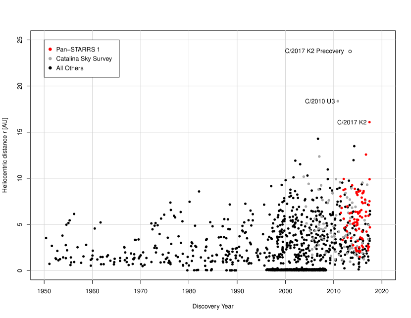
Figure 1: Heliocentric distances at time of discovery of 2096 long-period comets discovered after 1950. The points near 0 au starting in 1996 are SOHO sun-grazing or impacting comets. The density of points increased significantly after 1996 when many of the major moving object sky surveys began.

To compare to the discovery distances for other long period (LP) comets, we searched the Minor Planet Center comet database CmtObs.dat of all long-period comet observations back to 1950 (see Fig. 1). We assumed that the discovery is the date of the earliest observation. For some comets, the earliest MPC observations might be pre-discovery recoveries (precoveries), so comets at $r>10$ au at their first observation were investigated further to remove precovery observations. Then we used OpenOrb (Granvik et al., 2009) to compute the heliocentric distance at time of discovery. Only C/2010 U3 (Boattini) was discovered farther from the Sun, at 18.4 au. Thus, C/2017 K2 is the second most distant discovery of an active comet, and pre-discovery observations at $r=23.75$ au represent the largest distance at which an active comet has been observed approaching perihelion. Most of the historically bright LP comets discovered prior to 1950 were discovered much closer to the sun, with only a few exceptions at $r>5$ au, and none were discovered inbound at distances greater than 6.5 au (Roemer, 1962). There were a few bright historical comets for which dust-dynamical models suggest activity began as far out as 30 au (Sekanina, 1975).

The proliferation of all-sky surveys such as LINEAR (Stokes et al., 2000), Spacewatch (Gehrels & Jedicke, 1996), the Catalina Sky Survey (CSS) (Larson, 2007), LONEOS (Bowell et al., 1995), and NEAT (Pravdo et al., 1999) in the mid-1990s, followed by Pan-STARRS1 (Kaiser et al., 2010; Chambers et al., 2017) in 2010 has resulted in a rapid increase in the discovery of faint active comets at increasingly large heliocentric distances (Fig. 1). Inbound comets, being heated for the first time, provide unique insights into the mechanisms of comet activity.

2 Observations and Data Reduction

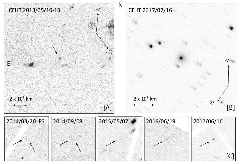
Figure 2: Composite images of C/2017 K2. [A] This 4200 sec composite (100$\times$100^′′) used the 7 best u-band CFHT images from 2013 May obtained from the CADC archive. [B] 2017 July 16 CFHT $r$-band composite with total exposure 720 sec. The image is 100^′′ on a side. The coma extends $\sim$3.5$\times$10⁵ km toward the W. The negative of the heliocentric velocity (-v) and the extended Sun-target vector or anti-solar direction are shown. [C] Composite images from the PS1 archive for several dates. All are $i$-band, except the first, which is $r$-band. All images are 1$\times$$10^{6}$ km on a side.

Photometry for C/2017 K2 was obtained using both the CFHT and Pan-STARRS1 (PS1) telescopes. The headers were used to download orbital elements from the Minor Planet Center, and the computed object location was used to determine which object in the frame corresponded to the target. Terapix tools (SExtractor) were used to produce multi-aperture and automatic aperture target photometry. To photometrically calibrate both telescopes we calculated a photometric zero point for each image using the Pan-STARRS database and published color corrections to translate photometric bands (Magnier et al., 2017; Chambers et al., 2017). Photometry and observing circumstances are presented in Table 1, and a selection of images is shown in Fig. 2.

2.1 Pan-STARRS1

A search for pre-discovery observations in the PS1 images taken between 2010 to 2017, resulted in almost 200 images at the comet’s location. The comet is visible in about half of the frames after 2014, while older images or images in narrower passbands are not deep enough to detect it. However, the astrometry from the positive detections constrains the ephemeris to less than one pixel over the entire arc. This allowed us to measure a lower magnitude limit in images where it was not visible.

We measured the photometry for these PS1 images using a 2$\farcs$5 radius aperture. When the comet was too faint and SExtractor was unable to locate it, the photometry was done by placing an aperture at the comet’s expected position. The data reported in Table 1 represent the weighted average magnitudes from all detections on a given night. Conversions to the SDSS photometric system used the transformations from Tonry et al. (2012). For images where SExtractor was unable to locate the comet, but it was visible to the observer, we confirmed that the measurements were of the comet by inspection. In all cases the comet appeared extended. We measured the curve of growth for frames where the comet was visible at high $S/N$ to estimate an aperture correction of $\Delta m$ = -0.63 mag to convert to a 5^′′ radius uniform aperture for comparison of all the data to the models in $\S$3.1. To obtain limiting magnitudes where the comet was not visible, we plotted on each field the mean-magnitudes of the stars from the PS1 PV3 catalog (which utilizes the best data reduction and calibration). The limiting magnitude in each field, at which stars were no longer visible, was at S/N$\approx 2$. Using only the observations available on the MPC website, the uncertainty in the orbit position (the long semi-major axis of the 1-$\sigma$ uncertainty ellipse) is $\pm$0$\farcs$15 for the entire period from 2010 to 2017. Including the new pre-discovery data found in the PS1 images, the error is even smaller for some periods. With a plate scale of 0$\farcs$25 per pixel, the positional uncertainty is $<$ 1 pixel in the images. For most frames the limiting magnitude was around $r$$\sim$$i$$\sim$21.3.

2.2 CFHT

We obtained additional images using the CFHT MegaCam wide-field imager, an array of forty 2048$\times$4612 pixel CCDs with a plate scale of 0$\farcs$187 per pixel and a 1.1 square degree FOV. The data were obtained through SDSS filters using queue service observing and were processed to remove the instrumental signature through the Elixir pipeline (Magnier & Cuillandre, 2004). The colors for this active LP comet are shown in Table 1 and are consistent with other active LP comets (Jewitt, 2015). We have converted the colors to a relative spectral reflectivity using

$$R_{\lambda}=\frac{10^{-0.4(m_{\lambda}-m_{\lambda\odot})}}{10^{-0.4(m_{o}-m_{o\odot})}}=\frac{N}{D}$$ (1)

$$\sigma_{R\lambda}=R_{\lambda}^{2}\left[\left(\frac{0.9212N\sigma_{\lambda}}{N}\right)^{2}+\left(\frac{0.9212D\sigma_{mo}}{D}\right)^{2}\right]^{0.5}$$ (2)

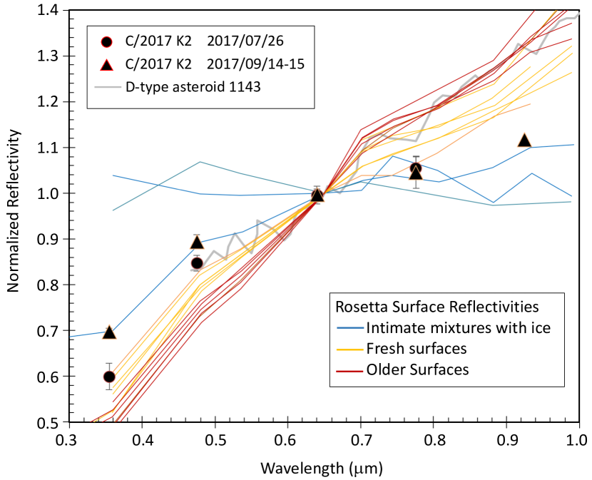
Figure 3: Spectral reflectivity of C/2017 K2 obtained on 2017 July 26 and 2017 September 14-15 (see Table 1) compared to reflectivities of different surface types on C/67P Churyumov-Gerasimenko from the OSIRIS imaging system (Fornasier et al., 2017).

Here $N$ and $D$ represent the numerator and denominator in Eq. (1), $m_{\lambda}$ is the magnitude in a specific filter $\lambda$, $\sigma_{\lambda}$ is the uncertainty on $m_{\lambda}$, $m_{o}$ is the reference bandpass that we normalize to, and $m_{\odot}$ is the absolute magnitude of the sun. For the SDSS filters we use $g_{\odot}$ = 5.12$\pm$0.02, $r_{\odot}$ = 4.69$\pm$0.03, $i_{\odot}$ = 4.57$\pm$0.03, and $z_{\odot}$ = 4.60$\pm$0.03. We normalized the spectral reflectivities to $\lambda$=0.65 $\mu$m. The spectral reflectivity is shown in Fig. 3 in comparison with the reflectivity from several regions from the surface of comet 67P/Churyumov-Gerasimenko as imaged by the $Rosetta$ OSIRIS instrument (Fornasier et al., 2017).

We used the Solar System Object Image Search tool at the Canadian Astronomy Data Centre (Gwyn et al., 2012) to search all archival data stored there for images that might have had pre-discovery detections of the comet. Eleven $u$-band exposures were found from 2013 May 10-13 obtained with Megacam on the CFHT for a total integration time of 6600 sec. These images were also processed by the Elixir pipeline. The comet is clearly visible at the expected position and appears diffuse. The magnitude of the comet was measured on the combination of the best 7 images giving $u=23.09\pm 0.17$. We used our measured ($u-r$)=2.333$\pm$0.055 color index to convert to $r$=20.76$\pm$0.23 (Table 1).

2.3 NEOWISE

The NEOWISE survey (Mainzer et al., 2014) observed C/2017 K2 during two visits. The first was for 76 exposures between 2017-03-27 17:35:44.627 UT and 2017-04-06 07:02:15.385 UT, with a mid-frame observing time of 2017-04-01 20:10:26.526 UT. The second visit was for 65 exposures between 2017-06-27 01:38:28.719 UT and 2017-07-08 20:27:56.365 UT with a mid-frame observing time of 2017-07-02 23:03:12.423 UT. The mid-frame heliocentric distances were $r$=15.8 au and $r$=16.4 au, respectively. The $W2$ band encompasses both the CO 1-0 and CO₂ $\nu_{3}$ emission bands. Because the ratio of the CO₂ to CO $g$-factors is $\sim$11.2 (Bockelee-Morvan & Crovisier, 1989), a given flux implies a much higher production rate for CO than CO₂. These visits showed no significant detections, and using the techniques described in Bauer et al. (2015) yielded 3-$\sigma$ upper CO production rate limits of $Q_{CO}<$ 1.6$\times$10²⁸ and $Q_{CO}<$ 1.0$\times$10²⁸ molecules per second respectively, and upper CO₂ production limits of $Q_{CO2}<$ 1.4$\times$10²⁷ and $Q_{CO2}<$ 8.9$\times$10²⁶ molecules per second respectively.

3 Analysis

3.1 Sublimation Models

We used a surface ice sublimation model (Meech et al., 1986) to investigate the activity for comet C/2017 K2. The model computes the amount of gas sublimating from an icy surface exposed to solar heating, as described in detail in Meech et al. (2017). The total brightness within a fixed aperture combines radiation scattered from both the nucleus and the dust dragged from the nucleus in the escaping gas flow, assuming a dust to gas mass ratio of 1. This type of model can distinguish between H₂O, CO, and CO₂ driven activity. The model free parameters include: nucleus radius, albedo, emissivity, nucleus density, dust properties, and fractional active area. When there is information about some of the parameters, it is possible to constrain many of the others.

Because C/2017 K2 is a recent discovery, none of the model parameters are constrained. However, based on typical values for other comets seen in-situ and from the ground (Meech, 2017b), we assumed the following: nucleus albedo, $p_{v}$=0.04, emissivity, $\epsilon$=0.9, nucleus phase function, $\beta$=0.04 mag deg^-1, coma phase function, $\beta_{c}$=0.02 mag deg^-1, and nucleus density, $\rho_{N}$=400 kg m^-3, and an average dust size of 2 $\mu$m. With steep power law size distributions for grains ranging in size between 0.1$\mu$m-mm, the small particles dominate (Fulle et al., 2016). The grain sizes can’t be modeled using a dust-dynamical techniques because this comet has severe projection effects (i.e. we are looking straight down the tail). With knowledge of the nucleus size, the fractional active area can be fit. However, as this comet was discovered active, we have no a priori knowledge of the nucleus size thus the only parameter we can constrain is the effective surface area of the sublimating ice for each volatile.

We ran a suite of models with a range of nucleus sizes and found that for a radius $R_{N}$=80 km the model brightness (nucleus+coma) approached that of the photometry–unrealistic given that all of the images showed a dust coma, indicating activity. We thus use $R_{N}$=80 km as an upper limit to the nucleus size assuming an albedo $p_{v}$=0.04.

Assuming that the CO outgassing surface area remains constant, with no CO₂ contribution through perihelion, and that the fractional nucleus surface area for H₂O-ice sublimation is 4%-typical of other nuclei without icy halos (A’Hearn et al., 1995), we can infer the minimum nucleus radius. Data for the $\sim$30 comets with high-quality simultaneous H₂O and CO production rate ($Q$) measurements show that at perihelion and within 2 au, when water-sublimation is strong, the ratios of Q_CO/Q_H2O are below 30% (Paganini et al., 2014; Meech, 2017b). Fitting models with a range of nucleus sizes to calculate the production rates for H₂O and CO at perihelion, we rule out nuclei with $R_{N}<$14 km because they would require Q_CO/Q${}_{H2O}\geq$30% and an active surface fraction of 0.092% for CO sublimation. This suggests that the C/2017 K2 nucleus with $14<R_{N}<80$ km could be as large as C/1995 O1 (Hale-Bopp) which had $R_{N}\sim 30\pm 10$ km (Fernández, 2002).

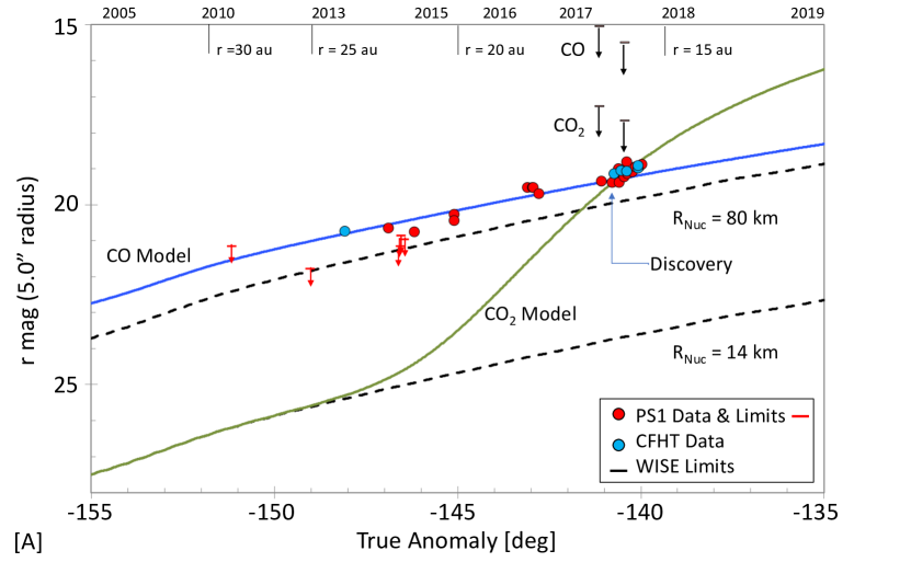
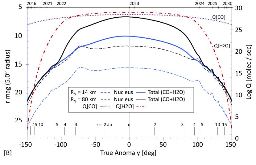
Figure 4: [A] Best fit CO-sublimation model (blue) compared to the photometry in Table 1 for our two limiting nucleus sizes. A CO₂ model (green) for a 14 km-radius nucleus consistent with the photometry at the time of discovery is also shown, but is inconsistent with the earlier PS1 data. The upper limiting model magnitudes that correspond to the flux limits from the WISE observatory are also shown. [B] Run out of the CO-sublimation models for 2 nucleus sizes assuming constant sublimating area for both H₂O and CO. Under this assumption, and if there are no seasonal effects, this plot can be used to estimate the comet’s brightness and H₂O and CO production rates. These rates are shown for the $R_{N}$ = 14 km nucleus (dotted and dash-dot lines). For the $R_{N}$ = 80 km nucleus case the $Q_{CO}$ curve shifts by -0.37 and the $Q_{H2O}$ curve shifts by +1.51 in log.

Figure 4A shows the best fit model for a nucleus radius of 14 km for sublimation from CO or CO₂, forced to match the photometric data at the time of discovery at TA=-140.8^∘. We also show a fit for an 80 km radius nucleus. The data from 2017 May to September show insufficient range along the orbit (TA) to distinguish between sublimation from CO or CO₂ as a driver of the activity. At these distances, there is no contribution from H₂O sublimation. However, the pre-discovery data from PS1, and the archival CFHT data show very clearly that only the CO-sublimation model can reproduce the photometry. Changing the nucleus size increases or decreases the nucleus contribution to the total brightness, but at these distances has no effect on the shape of the light curve. We ran models for CO and CO₂ sublimation that produced gas flows consistent with the gas production rate limits obtained from the WISE data (see $\S$ 2.3) and have plotted the corresponding expected limits on the total brightness in the figure. According to the best fit models, the maximum grain size that could be lifted off at these distances for CO₂ sublimation is $\sim$2 $\mu$m, and for CO sublimation a few 100 $\mu$m. The dust grain size we used for the models is well below this limit.

4 Discussion

The PS1 limiting magnitudes at $\sim$30 au and the precovery data until discovery are consistent with a steady sublimation from the surface. The model is brighter than the limit at TA=-149^∘, but this could reflect a lower comet brightness possibly due to nucleus rotation. The difference is not significant enough to interpret this as a sublimation decrease.

There are several possible mechanisms for activity at these large distances. The equilibrium sublimation temperatures of the most abundant ices that can drive activity, CO, CO₂ and H₂O, are 25K, 80K and 160K, respectively. Sublimation rate is a non-linear function of temperature, and can occur at low rates at large distances. The distance at which surface-ice sublimation becomes effective at driving comet activity is when the gas flow lifts sufficient dust from the surface to be detected from Earth. For water this is within the distance of Jupiter; for CO₂, between Saturn and Uranus; and for CO, within the Kuiper belt (Meech et al., 2009). Volatiles condensing below 100K can also be trapped in amorphous water ice and their release occurs as the ice is heated and undergoes restructuring through annealing or the amorphous-to-crystalline ice transition. This transition begins around 120K and annealing begins at temperatures as low as 37K. CO is the only abundant cometary volatile that can reproduce the C/2017 K2 lightcurve shape from sublimation at these distances. It is not possible to distinguish between other distant activity mechanisms without denser heliocentric light curve data of higher precision, including observations at larger distances.

The comet’s spectral reflectivity falls within the envelope of the different regions on comet 67P (Fig. 3). Many regions on comet 67P were similar to or redder than typical D-type asteroids, and were dominated by organic-rich refractory material. It was observed that 67P became spectrally less red overall as it approached perihelion and dust was removed, exposing underlying water ice (Fornasier et al., 2017). The spatially resolved spectral reflectivities show that newly exposed materials were less red, while in regions with spectroscopic signature of water-ice frost, the spectrum became progressively bluer, with the flat reflectivities having 20-32% water-ice frost. The reflectivity slope of C/2017 K2 is more consistent with 67P surfaces that contained some water-ice frost. This could be the result of strong sublimation from near-surface CO for many years.

In order to provide some guidance to observers who may want to plan observing runs to watch the development of activie, in Fig. 4B we run the models for both limiting nucleus cases through perihelion out to 25 au post-perihelion. On the assumption that the fractional active areas of CO and H₂O do not change and there are no seasonal effects, the peak brightness of the comet should be between magnitude 7-11 through a 5^′′ aperture.

On the right side of Fig. 4B we show the corresponding estimated production rates for both volatiles. To estimate the detectability of volatile species and D/H isotopologues at infrared wavelengths by ground-based observatories, we use a Figure of Merit (FoM). FoM is used to gauge the strength of molecular line emission. Traditionally, FoM = 10²⁹ $\times$ Q $\times$r^-1.5$\times$$\Delta$^-1, where Q is the H₂O production rate (molecules s^-1) predicted by our models, and $r$ and $\Delta$ are heliocentric and geocentric distance, in au. Typically, for a comet with FoM $\geq$ 0.08 we expect to measure H₂O and for FoM $\geq$ 2 we expect to unambiguously detect HDO. Adopting the H₂O production rates predicted for the lower and upper $R_{N}$ limits of 14 km and 80 km, the FoM predicts that H₂O is detectable inside $r$$\sim$2.1 au and $\sim$3.4 au, respectively. If $R_{N}$ is 80 km, then a D/H measurement would be possible inside $r$$\sim$2.1 au (i.e. from about early September 2022 through late March 2023). Of course, it is highly likely that the mixing ratios will not remain constant; this is just a guide for planning observations.

The James Webb Space Telescope ($JWST$) will facilitate high SNR spectra in the 2–5$\mu$m region to characterize the chemical composition of comets through the resolved spectral signatures of H₂O, CO, and CO₂. However, $JWST$ pointing limitations restrict observations to solar elongations between 85^∘-135^∘, limiting the windows of observability. According to the current $JWST$ launch window estimates, the earliest we can observe the comet will be at $\sim$ 11 au. Adopting our model predicted CO production rate of $\sim$ 10²⁶ molecules sec^-1 at r $\sim$ 11 au, one hour of on-source integration yields a spectrum with a S/N$\sim$50 across the CO₂ and CO wavelength region using NIRSpec with a medium resolution G395M filter. $JWST$ observations at this distance would provide the first fully resolved medium resolution spectral signatures of CO and CO₂ fundamental vibration bands in a pre-perihelion comet beyond 6.2 au.

Figure 1 shows that all-sky surveys are finding more LP comets, and at larger distances. Since 2010, of the $\sim$300 LP comets discovered, PS1 (31.3%; shown as the red dots in Fig. 1) and CSS (26.1%) are dominating the discoveries. Surprisingly, no survey or group is yet dominant for $r>10$ au. Since 2000 there have been 13 comets discovered beyond this distance. While some are discovered by surveys (PS1, Catalina, LONEOS, NEAT), others are discovered in deep targeted searches for distant trans-Neptunian objects. The Pan-STARRS2 telescope (Morgan et al., 2012) will double the survey power of PS1 beginning in 2018. When the Large Synoptic Survey Telescope (LSST) begins its survey in 2023, we expect an explosion in distant LP comet discoveries that will enable a new understanding of cometary physics. With these surveys we may finally obtain observational confirmation of the activity that was predicted for historical comets as far out as 30 au (Sekanina, 1975).

Acknowledgements KJM, JTK, and JVK acknowledge support through awards from the National Science Foundation AST1413736 and AST1617015. RJW acknowledges support by the National Aeronautics and Space Administration under grant NNX14AM74G issued through the SSO Near Earth Object Observations Program. LD acknowledges support by NASA under grants NNX12AR55G and NNX14AM74G.

Based also in part on observations obtained with MegaPrime/MegaCam, a joint project of CFHT and CEA/DAPNIA, at the Canada-France-Hawaii Telescope (CFHT) which is operated by the National Research Council (NRC) of Canada, the Institute National des Science de l’Univers of the Centre National de la Recherche Scientifique (CNRS) of France, and the University of Hawai’i. This research used the facilities of the Canadian Astronomy Data Centre operated by the National Research Council of Canada with the support of the Canadian Space Agency.

Note added in Proof – During review, a paper by Jewitt et al. (2017) on C/2017 K2 was published. Our nucleus radius lower limit is not in disagreement with the upper limit they presented. Ours is a spherical equivalent radius, and their estimate is from an instantaneous measurement. Nucleus axis ratios have been seen as high as 3.3 from the EPOXI mission. The technique of using high-resolution HST measurements and coma removal typically produces agreement within $\pm$10-50% of the spherical equivalent radius.

Table 1: Observing Geometry and Photometry

UTDate	JD	$r$	$\Delta$	$\alpha$	TA	Filt	# Images	mag$\pm$$\sigma$	rmag$\pm$$\sigma$	Color/Comment
PanSTARRS1 data
2010/06/04	5352.10123	28.665	28.754	2.017	-151.16	ip1	2	$<$21.0$\pm$0.3	$<$21.2$\pm$0.3	Limiting mag
2012/08/07	6146.81325	25.061	25.146	2.306	-149.01	rp1	2	$<$21.8$\pm$0.3	$<$21.8$\pm$0.3	Limiting mag
2014/06/14	6821.46247	21.802	21.829	2.666	-146.54	ip1	3	$<$21.0$\pm$0.3	$<$21.2$\pm$0.3	Limiting mag
2014/06/13	6822.51886	21.797	21.824	2.667	-146.54	ip1	3	$<$20.7$\pm$0.3	$<$20.9$\pm$0.3	Limiting mag
2014/07/05	6844.27742	21.688	21.729	2.681	-146.45	ip1	2	$<$20.8$\pm$0.3	$<$21.0$\pm$0.3	Limiting mag
2014/03/20	6737.07683	22.221	22.202	2.569	-146.88	rp1	2	20.67$\pm$0.30	20.67$\pm$0.30
2014/09/08	6908.76850	21.364	21.430	2.692	-146.17	ip1	4	20.60$\pm$0.05	20.77$\pm$0.05
2015/05/06	7149.01152	20.138	20.122	2.871	-145.09	ip1	4	20.10$\pm$0.04	20.28$\pm$0.04
2015/05/07	7150.00904	20.133	20.117	2.872	-145.08	ip1	4	20.27$\pm$0.05	20.45$\pm$0.05
2016/05/27	7536.02124	18.088	18.052	3.211	-143.07	rp1	4	19.53$\pm$0.04	19.53$\pm$0.04
2016/06/19	7558.88673	17.963	17.938	3.242	-142.94	ip1	3	19.37$\pm$0.08	19.54$\pm$0.08
2016/06/21	7560.93624	17.952	17.928	3.245	-142.93	ip1	2	19.37$\pm$0.06	19.54$\pm$0.06
2016/07/18	7587.88946	17.805	17.803	3.270	-142.77	ip1	4	19.53$\pm$0.05	19.71$\pm$0.05
2017/04/10	7854.05173	16.322	16.280	3.519	-141.06	ip1	4	19.19$\pm$0.07	19.36$\pm$0.07
2017/05/21	7894.91140	16.089	16.019	3.604	-140.77	wp1	4	19.45$\pm$0.03	19.39$\pm$0.03	Discovery
2017/06/16	7920.97821	15.940	15.874	3.651	-140.59	ip1	4	18.85$\pm$0.04	19.02$\pm$0.04
2017/06/25	7929.91675	15.888	15.828	3.666	-140.52	wp1	4	19.19$\pm$0.03	19.13$\pm$0.03
2017/08/06	7971.88255	15.646	15.638	3.715	-140.21	ip1	4	18.94$\pm$0.05	19.11$\pm$0.05
2017/08/17	7982.77565	15.583	15.594	3.721	-140.13	wp1	4	19.02$\pm$0.01	18.97$\pm$0.02
2017/08/30	7995.76736	15.508	15.542	3.725	-140.03	ip1	4	18.78$\pm$0.04	18.96$\pm$0.04
2017/09/07	8003.77876	15.461	15.511	3.724	-139.96	ip1	4	18.72$\pm$0.04	18.90$\pm$0.04
2017/06/16	7920.95557	15.940	15.874	3.651	-140.59	rp1	4	18.96$\pm$0.06	19.14$\pm$0.06
2017/07/05	7939.88379	15.831	15.779	3.681	-140.45	rp1	2	18.94$\pm$0.14	19.11$\pm$0.14
2017/07/07	7941.90196	15.819	15.770	3.684	-140.43	rp1	4	19.24$\pm$0.11	19.41$\pm$0.11
2017/07/15	7949.87944	15.773	15.733	3.694	-140.37	rp1	4	18.82$\pm$0.06	19.00$\pm$0.06
2017/07/17	7951.90526	15.762	15.724	3.696	-140.36	rp1	4	19.15$\pm$0.20	19.33$\pm$0.20
CFHT Archival data from CADC
2013/05/12	6424.61132	23.744	23.767	2.436	-148.07	u	7	23.09$\pm$0.17	20.76$\pm$0.23
CFHT new data
2017/05/24	7898.05595	16.071	16.000	3.610	-140.75	w	1	19.292$\pm$0.007	19.237$\pm$0.007
2017/05/28	7901.92345	16.049	15.978	3.617	-140.72	g	1	19.673$\pm$0.015
2017/05/28	7901.92345	16.049	15.978	3.617	-140.72	r	1	19.155$\pm$0.015	19.155$\pm$0.015	(g-r) = 0.52$\pm$0.02
2017/06/24	7928.97060	15.894	15.833	3.665	-140.53	g	1	19.539$\pm$0.012
2017/06/24	7928.97049	15.894	15.833	3.665	-140.53	r	1	19.067$\pm$0.013	19.067$\pm$0.013	(g-r) = 0.47$\pm$0.02
2017/07/16	7950.83854	15.768	15.729	3.695	-140.37	r	12	19.081$\pm$0.004	19.081$\pm$0.004
2017/07/25	7990.80063	15.768	15.729	3.695	-140.37	g	1	19.567$\pm$0.011		(g-r) = 0.56$\pm$0.02
2017/07/25	7990.80285	15.768	15.729	3.695	-140.37	r	1	19.007$\pm$0.012	19.007$\pm$0.012
2017/07/26	7991.80022	15.537	15.562	3.724	-140.06	u	2	21.260$\pm$0.054		(u-r) = 2.33$\pm$0.06
2017/07/26	7991.80602	15.531	15.558	3.724	-140.06	g	1	19.513$\pm$0.013		(g-r) = 0.59$\pm$0.02
2017/07/26	7991.80407	15.537	15.562	3.724	-140.06	r	3	18.927$\pm$0.008	18.927$\pm$0.008
2017/07/26	7991.80889	15.531	15.558	3.724	-140.06	i	2	18.758$\pm$0.013		(r-i)  = 0.17$\pm$0.02
2017/09/14	8010.74649	15.421	15.483	3.723	-139.91	g	4	19.483$\pm$0.005		(g-r) = 0.55$\pm$0.01
2017/09/14	8010.74282	15.421	15.483	3.723	-139.91	r	2	18.932$\pm$0.009	18.932$\pm$0.009
2017/09/14	8010.74230	15.421	15.483	3.723	-139.91	i	6	18.761$\pm$0.008		(r-i)  = 0.17$\pm$0.01
2017/09/14	8010.75793	15.421	15.483	3.723	-139.91	z	4	18.721$\pm$0.024		(r-z) = 0.21$\pm$0.03
2017/09/15	8011.72479	15.415	15.479	3.723	-139.90	u	3	20.995$\pm$0.039		(u-r) = 2.12$\pm$0.04
2017/09/15	8011.74031	15.415	15.479	3.723	-139.90	g	5	19.413$\pm$0.004		(g-r) = 0.54$\pm$0.01
2017/09/15	8011.75514	15.415	15.479	3.723	-139.90	r	2	18.873$\pm$0.007	18.873$\pm$0.007

References

- A’Hearn et al. (1995) A’Hearn, M. F., Millis, R. C., Schleicher, D. O., Osip, D. J., & Birch, P. V. 1995, Icarus, 118, 223
- Bauer et al. (2015) Bauer, J. M., Stevenson, R., Kramer, E., et al. 2015, ApJ, 814, 85
- Bockelee-Morvan & Crovisier (1989) Bockelee-Morvan, D., & Crovisier, J. 1989, A&A, 216, 278
- Bowell et al. (1995) Bowell, E., Koehn, B. W., Howell, S. B., Hoffman, M., & Muinonen, K. 1995, Bulletin of the American Astronomical Society, 27, 01.10
- Chambers et al. (2017) Chambers, K. C., et al. 2017, https://arxiv.org/abs/1612.05560
- Fernández (2002) Fernández, Y. R. 2002, Earth Moon and Planets, 89, 3
- Fornasier et al. (2015) Fornasier, S., Hasselmann, P. H., Barucci, M. A., et al. 2015, A&A, 583, A30
- Fornasier et al. (2017) Fornasier, S., Feller, C., Lee, J.-C., et al. 2017, MNRAS, 469, S93
- Fulle et al. (2016) Fulle, M., Marzari, F., Della Corte, V., et al. 2016, ApJ, 821, 19
- Gehrels & Jedicke (1996) Gehrels, T., & Jedicke, R. 1996, Earth Moon and Planets, 72, 233
- Granvik et al. (2009) Granvik, M., Virtanen, J., Oszkiewicz, D., & Muinonen, K. 2009, Meteoritics and Planetary Science, 44, 1853
- Gwyn et al. (2012) Gwyn, S. D. J., Hill, N., & Kavelaars, J. J. 2012, PASP, 124, 579
- Kaiser et al. (2010) Kaiser, N., Burgett, W., Chambers, K., et al. 2010, Proc. SPIE, 7733, 77330E
- Jewitt (2015) Jewitt, D. 2015, AJ, 150, 201
- Jewitt et al. (2017) Jewitt, D., Hui, M.-T., Mutchler, M., et al. 2017, ApJ, 847, L19
- Larson (2007) Larson, S. 2007, Current NEO Surveys, in: Valsecchi, G.B., Vokrouhlicky, D. (Eds)., IAU Symposium, vol. 236, pp. 323-328.
- Magnier & Cuillandre (2004) Magnier, E. A., & Cuillandre, J.-C. 2004, PASP, 116, 449
- Magnier et al. (2017) Magnier, E. A., et al. 2017, https://arxiv.org/abs/1612.05242
- Mainzer et al. (2014) Mainzer, A., Bauer, J., Cutri, R. M., et al. 2014, ApJ, 792, 30
- Meech (2017b) Meech, K. J. 2017b, Philosophical Transactions of the Royal Society of London Series A, 375, 20160247
- Meech et al. (1986) Meech, K. J., Jewitt, D., & Ricker, G. R. 1986, Icarus, 66, 561
- Meech et al. (2009) Meech, K. J., Pittichová, J., Bar-Nun, A., et al. 2009, Icarus, 201, 719
- Meech et al. (2017) Meech, K. J., Schambeau, C. A., Sorli, K., et al. 2017, AJ, 153, 206
- Morgan et al. (2012) Morgan, J. S., Kaiser, N., Moreau, V., Anderson, D., & Burgett, W. 2012, Proc. SPIE, 8444, 84440H
- Paganini et al. (2014) Paganini, L., Mumma, M. J., Villanueva, G. L., et al. 2014, ApJ, 791, 122
- Pravdo et al. (1999) Pravdo, S. H., Rabinowitz, D. L., Helin, E. F., et al. 1999, AJ, 117, 1616
- Roemer (1962) Roemer, E. 1962, PASP, 74, 351
- Sekanina (1975) Sekanina, Z. 1975, Icarus, 25, 218
- Stokes et al. (2000) Stokes, G. H., Evans, J. B., Viggh, H. E. M., Shelly, F. C., & Pearce, E. C. 2000, Icarus, 148, 21
- Tonry et al. (2012) Tonry, J. L., Stubbs, C. W., Lykke, K. R., et al. 2012, ApJ, 750, 99