LinXGBoost: Extension of XGBoost to
Generalized Local Linear Models

Abstract

XGBoost is often presented as the algorithm that wins every ML competition. Surprisingly, this is true even though predictions are piecewise constant. This might be justified in high dimensional input spaces, but when the number of features is low, a piecewise linear model is likely to perform better. XGBoost was extended into LinXGBoost that stores at each leaf a linear model. This extension, equivalent to piecewise regularized least-squares, is particularly attractive for regression of functions that exhibits jumps or discontinuities. Those functions are notoriously hard to regress. Our extension is compared to the vanilla XGBoost and Random Forest in experiments on both synthetic and real-world data sets.

1 Introduction

Most competitors in ML jump straight to XGBoost, Chen und Guestrin (2016), an implementation of the gradient boosting algorithm, because of its speed and accurate predictive power. Part of XGBoost amazing speed must be ascribed to the fact that predictions are piecewise constant. From a modeling perspective, this might certainly be the right thing to do in high-dimensional input spaces, but if the number of features is low, a piecewise linear model is likely to yield a better predictive performance.

This is best seen on a one-dimensional function. Consider the synthetic HeavySine function, Donoho und Johnstone (1995), a sinusoid of period 1 with two jumps, at $t_{1}=.3$ and $t_{2}=.72$:

$$f(t)=4\sin(4\pi t)-\text{sign}(t-0.3)-\text{sign}(0.72-t)$$ (1)

Given enough trees, XGBoost can adequately fit the noisy data set, Figure 1, left. If we constrain XGBoost to a single tree and further regularize the model to prevent over-fitting, the piecewise constant nature of the predictions is clearly revealed, Figure 1, middle. A single tree with a linear model at the leaves produces visually far better results, Figure 1, right. To get better results in terms of the NMSE performance metric, more trees are needed though. By adding quadratic terms, we can even get superior results.

Figure 1: Regression of the HeavySine function based on 201 noisy samples (the noise is Gaussian with zero mean and variance $\sigma^{2}=0.05$). Left: XGBoost with default setting except that the learning rate is reduced to 0.1 and the number of trees boosted to 50. Middle: XGBoost using a single tree. Right: LinXGBoost using also a single tree. In the middle and right plots, both XGBoost and LinXGBoost share the same tree maximum depth, 30, and regularization term on the number of leaves $\gamma=3$ and L2 regularization term on weights $\alpha=0$.

A piecewise (constant or linear) model is particularly suited for the regression of functions that exhibit jumps or discontinuities. Finding jumps in otherwise smooth functions is a notoriously hard challenge. It usually involves the derivation of criteria for choosing the number and placement of the jumps, Lee (2002). Even Bayesian models treat exclusively jumps in one-dimensional signals, i.e. time series, Adams und MacKay (2007).

A piecewise linear model is appropriate for functions whose smoothness is input-dependent. There are well established techniques to regress functions whose smoothness does not vary (e.g. the Nadaraya-Watson kernel estimator or Gaussian processes, both with a fixed bandwidth). While convenient, the assumption that the smoothness is input-independent is rarely realistic. Extensions to model functions with varying length-scales are not trivial (e.g. adaptive Nadaraya-Watson kernel estimator or non-stationary Gaussian processes). Nevertheless, this is essential in many fundamental problems. Modeling terrain surfaces, for instance, given sets of noisy elevation measurements is even more challenging since it requires the ability to balance smoothing against the preservation of discontinuities (see e.g. Plagemann u. a. (2008)).

At the core of gradient boosting are regression trees. A regression tree decomposes the input space into subdomains. This is reminiscent of the domain decomposition approach to regress non-stationary functions, Park u. a. (2011). In each input subdomain, the function can be approximately regarded as stationary. Therefore, local regression is applied in each subdomain with a fixed length-scale or bandwidth. But this results in discontinuities in prediction on boundaries of the subdomains, Park und Huang (2016). To mitigate this drawback, the assignment of data points to models can also be soft: The assignments are treated as unobserved random variables, Rasmussen und Ghahramani (2002). Because of the uncertainty in the assignments, discontinuities in predictions are smoothed out.

Domain decomposition is however rarely done in a principled way: In Kim u. a. (2005), the uncertainty in the number of disjoint regions, their shapes and the model within regions was dealt with in a fully Bayesian fashion. However, this feat has a price: It is fairly involved and slow (because of Reversible jump MCMC) and limited to small feature space dimensions (because of the Voronoi tessellation).

Finding the right size of the local region for linearization is a problem faced in Locally Weighted Learning, Englert (2012). Meier u. a. (2014) developed a Bayesian localized regression algorithm. The local models were added incrementally but not in a fully consistent manner.

Though XGBoost is not Bayesian, the trees are grown and the scores at the leaves are chosen in a principled way: To minimize an objective function. Consequently, XGBoost can automatically captured jumps and discontinuities, Figure 2, left. Through the extension to local linear models, we make it able to additionally better model smooth functions with varying length-scales using fewer trees, Figure 2, middle and right.

Figure 2: Left: Regression of a noisy data set from a piecewise constant function. XGBoost can automatically infer the right number of partitions using a single tree. Middle: Regression of a noisy data set from a piecewise linear function. Because XGBoost predictions are piecewise constant, we are forced to boost the number of trees (and so reduce the learning rate) to fit the data. The tree was not regularized: A strong regularization would lead to piecewise constant predictions. Right: LinXGBoost using a single tree provides a much better match. Notice that the tree was regularized.

It is not possible to natively handle categorical features; as in XGBoost, they must be encoded into numerical vectors using e.g. one-hot encoding.

Notice that plugging-in higher-order models at the tree leaves was advocated by Torgo (1997) to produce local regression trees. He acknowledged that this strategy brings significant gains in terms of prediction accuracy at the cost of an increase of computation time.

2 The vanilla XGBoost

We follow and borrow material from the clear-cut presentation in Chen (2014). We refer to this presentation for further details.

XGBoost implements a Boosting algorithm. Boosting algorithms belongs to ensemble machine learning methods. Specifically, they iteratively add predictors that focus on improving the current model, and this is achieved by modifying the learning problem (the objective in XGBoost) between iterations, see e.g. Elith u. a. (2008). Hence, boosting algorithms greedily approximate a function.

The predictors XGBoost builds are regression trees. A regression tree has decision rules and scores at the leaves. It is a function since it maps features (the attributes) to values (the scores). The prediction at $\boldsymbol{x}_{*}$ is given by

$$\hat{y}=\sum_{k=1}^{K}{f_{k}(\boldsymbol{x}_{*})}$$ (2)

assuming we have $K$ trees. $f_{k}\in\mathcal{F}$ where $\mathcal{F}$ is the space of functions containing all regression trees. The set of parameters is thus $\boldsymbol{\theta}=\{f_{1},\cdots,f_{K}\}$. Instead of learning weights as in linear regression or logistic regression, we are learning functions.

In XGBoost, the learning of functions is done by defining an objective to minimize:

$$Obj=\sum_{i=1}^{n}{\ell(y_{i},\hat{y}_{i})}+\sum_{k=1}^{K}{\Omega_{k}(f_{k})}$$ (3)

where $\hat{y}_{i}$ is the prediction and $y_{i}$ the observation at $\boldsymbol{x}_{i}$ for $i=1,\cdots,n$. $\ell(\cdot,\cdot)$ designates a loss function. The first term is the training loss, the second penalizes the complexity of trees.

In XGBoost, the objective at step $t$ is defined as

$$Obj^{(t)} = \sum_{i=1}^{n}{\ell(y_{i},\hat{y}_{i}^{(t)})}+\sum_{k=1}^{t}{\Omega_{k}(f_{k})}$$ (4)

$$= \sum_{i=1}^{n}{\ell(y_{i},\hat{y}_{i}^{(t-1)}+f_{t}(\boldsymbol{x}_{i}))}+\sum_{k=1}^{t}{\Omega_{k}(f_{k})}$$ (5)

$f_{t}(\boldsymbol{x}_{i})$ can be thought of as a perturbation (the residual), and so the loss is, to second-order accuracy:

$$\ell(y_{i},\hat{y}_{i}^{(t-1)}+f_{t}(\boldsymbol{x}_{i}))\approx\ell(y_{i},\hat{y}_{i}^{(t-1)})+g_{i}f_{t}(\boldsymbol{x}_{i})+\frac{1}{2}h_{i}f_{t}(\boldsymbol{x}_{i})^{2}$$ (6)

where $g_{i}$ (resp. $h_{i}$) is the first (resp. second) derivative of the loss w.r.t. its second argument evaluated at $(y_{i},\hat{y}_{i}^{(t-1)})$. For the square loss, $\ell(y_{i},\hat{y})=(y_{i}-\hat{y})^{2}$, we have $g_{i}=2(\hat{y}_{i}^{(t-1)}-y_{i})$ and $h_{i}=2$. In that particular case, the approximation is exact.

Removing the constant terms, we get

$$Obj^{(t)}=\sum_{i=1}^{n}{[g_{i}f_{t}(\boldsymbol{x}_{i}))+\frac{1}{2}h_{i}f_{t}(\boldsymbol{x}_{i})^{2}]}+\Omega_{k}(f_{t})$$ (7)

with

$$\Omega_{k}(f_{t})=\gamma T+\frac{1}{2}\lambda\sum_{k=1}^{T}{w_{k}^{2}}$$ (8)

to control the complexity of the tree. Notice that the number of leaves $T$ and the scores of the tree at the leaves $w_{k}$ ought to be indexed by $t$ to refer to the $t$-th iteration.

Assuming that the tree structure is known, it is possible to derivative the optimal weights. We have $f_{t}(\boldsymbol{x})=w_{q(\boldsymbol{x})}$ where $q(\boldsymbol{x})$ is the assignment function which assigns every data point to the $q(\boldsymbol{x})$-th leaf. Then define $I_{j}=\{i|q(\boldsymbol{x}_{i})=j\}$, the indices of all points that end up in the $j$-leaf. All data points in the same leaf share the same prediction. Consequently, the objective function can be recast as

$$Obj^{(t)}=\sum_{j=1}^{T}{\left[\left(\sum_{i\in I_{j}}{g_{i}}\right)w_{j}+\frac{1}{2}\left(\lambda+\sum_{i\in I_{j}}{h_{i}}\right)w_{j}^{2}\right]}+\gamma T$$ (9)

We can solve for the optimal weights $w_{j}^{*}$: Setting $G_{i}=\sum_{i\in I_{j}}{g_{i}}$ and $H_{i}=\sum_{i\in I_{j}}{h_{i}}$, we have

$$w_{j}^{*}=-\frac{G_{j}}{H_{j}+\lambda}$$ (10)

and so

$$Obj^{(t)}=-\frac{1}{2}\sum_{j=1}^{T}{\frac{G_{j}^{2}}{H_{j}+\lambda}}+\gamma T$$ (11)

The tree is grown in a top-down recursive fashion: For each feature in turn, XGBoost sorts the numbers and scans the best splitting point. The change of objective after a split is the gain:

$$gain=\frac{1}{2}\left[-\frac{(G_{L}+G_{R})^{2}}{H_{L}+H_{R}+\lambda}+\left(\frac{G_{L}^{2}}{H_{L}+\lambda}+\frac{G_{R}^{2}}{H_{R}+\lambda}\right)\right]-\gamma$$ (12)

The tree is grown until the maximum depth is reached. Then nodes with a negative gain are pruned out in a bottom-up fashion.

3 Linear models at the leaves

Instead of a score $w$, a leaf stores the weights of a linear model, $\boldsymbol{w}\in\mathbb{R}^{d+1}$ where $d$ is the dimension of the feature space, such that the local prediction at an unseen input $\boldsymbol{x}_{*}$ at the leaf is given by $\boldsymbol{w}^{T}\tilde{\boldsymbol{x}}_{*}$ where $\tilde{\boldsymbol{x}}_{*}=[\boldsymbol{x}_{*}\ ,\ 1]^{T}$.

This extension is natural:

• The simple model $\boldsymbol{w}^{T}\tilde{\boldsymbol{x}}$ captures both the linear and constant models.

• It is a form of locally weighted polynomial regression. However, instead of having a bandwidth controlling how much of the data is used to fit each local polynomial, all data points inside a specific hypervolume (the volume of feature space assigned to a leaf) are considered for model building. As in mixture of experts, the input space is divided into regions within which specific separate experts make predictions.

The objective at round $t$ changes from 7 to

$$Obj^{t)}=\sum_{i=1}^{n}{\left[g_{i}\tilde{\boldsymbol{x}}_{i}^{T}\boldsymbol{w}_{q(\boldsymbol{x}_{i})}+\frac{1}{2}\boldsymbol{w}_{q(\boldsymbol{x}_{i})}^{T}h_{i}\tilde{\boldsymbol{x}}_{i}\tilde{\boldsymbol{x}}^{T}_{i}\boldsymbol{w}_{q(\boldsymbol{x}_{i})}\right]}+\gamma T+\frac{1}{2}\lambda\sum_{j=1}^{T}{\boldsymbol{w}_{j}^{T}\boldsymbol{w}_{j}}$$ (13)

Regrouping by leaf, we get

$$Obj^{t)}=\sum_{j=1}^{T}{\left[\left(\sum_{i\in I_{j}}{g_{i}\tilde{\boldsymbol{x}}_{i}^{T}}\right)\boldsymbol{w}_{j}+\frac{1}{2}\boldsymbol{w}_{j}^{T}\left(\lambda\boldsymbol{I}_{d+1}+\sum_{i\in I_{j}}{h_{i}\tilde{\boldsymbol{x}}_{i}\tilde{\boldsymbol{x}}^{T}_{i}}\right)\boldsymbol{w}_{j}\right]}+\gamma T$$ (14)

By defining

$$\tilde{\boldsymbol{g}}^{T}_{j}=\sum_{i\in I_{j}}{g_{i}\tilde{\boldsymbol{x}}_{i}^{T}}\ ,\ \ \tilde{\boldsymbol{H}}_{j}=\sum_{i\in I_{j}}{h_{i}\tilde{\boldsymbol{x}}_{i}\tilde{\boldsymbol{x}}^{T}_{i}}$$ (15)

we have:

$$Obj^{t)}=\sum_{j=1}^{T}{\left[\tilde{\boldsymbol{g}}^{T}_{j}\boldsymbol{w}_{j}+\frac{1}{2}\boldsymbol{w}_{j}^{T}(\lambda\boldsymbol{I}_{d+1}+\tilde{\boldsymbol{H}}_{j})\boldsymbol{w}_{j}\right]+\gamma T}$$ (16)

Assuming the structure of the tree fixed, the optimal weights are given by

$$\boldsymbol{w}_{j}^{*}=-(\lambda\boldsymbol{I}_{d+1}+\tilde{\boldsymbol{H}}_{j})^{-1}\tilde{\boldsymbol{g}}_{j}$$ (17)

We have $\tilde{\boldsymbol{g}}_{j}=\tilde{\boldsymbol{X}}_{j}^{T}\boldsymbol{g}_{j}$ where $\tilde{\boldsymbol{X}}_{j}^{T}$ is the $(d+1)$-x-$|I_{j}|$ matrix whose columns are the $\tilde{\boldsymbol{x}}_{i}$. From the dyadic expansion, we can see that $\tilde{\boldsymbol{H}}_{j}=\tilde{\boldsymbol{X}}_{j}^{T}\boldsymbol{H}_{j}\tilde{\boldsymbol{X}}_{j}$ where $\boldsymbol{H}_{j}$ is a diagonal matrix with elements the $h_{i}$, $i\in I_{j}$. Because $h_{i}$ is the second derivative of a loss function, it is positive. Hence $\tilde{\boldsymbol{H}}_{j}$ is symmetric positive semi-definite and $\tilde{\boldsymbol{C}}_{j}=\lambda\boldsymbol{I}+\tilde{\boldsymbol{H}}_{j}$ is symmetric positive definite as long as $\lambda>0$. If so, $\tilde{\boldsymbol{C}}_{j}$ is Cholesky decomposed to solve for the optimal weights $\boldsymbol{w}_{j}^{*}$. If $\lambda=0$, then $\tilde{\boldsymbol{C}}_{j}$ is rank at most $d$, and so degenerate, if $|I_{j}|<d+1$ (less than $d+1$ input points fall into the leaf). In that particular situation, we fall back to the piecewise constant model.

$\tilde{\boldsymbol{C}}_{j}$ is a $(d+1)$-x-$(d+1)$ matrix where $d$ is the number of features: $\boldsymbol{x}\in\mathbb{R}^{d}$. If $d$ is much larger than the cardinality of $I_{j}$, then it might be convenient to use the Woodbury formula. Indeed, we have

$$\tilde{\boldsymbol{H}}_{j}=(\tilde{\boldsymbol{X}}_{j}^{T}\boldsymbol{H}_{j}^{\frac{1}{2}})(\tilde{\boldsymbol{X}}_{j}^{T}\boldsymbol{H}_{j}^{\frac{1}{2}})^{T}=\tilde{\boldsymbol{X}}_{j}^{h}\tilde{\boldsymbol{X}}_{j}^{hT}$$ (18)

Using the Woodbury formula, we get:

$$(\lambda\boldsymbol{I}_{d+1}+\tilde{\boldsymbol{H}}_{j})^{-1}=\frac{1}{\lambda}\boldsymbol{I}_{|I_{j}|}-\tilde{\boldsymbol{X}}^{h}\left(\boldsymbol{I}_{|I_{j}|}+\frac{1}{\lambda}\tilde{\boldsymbol{X}}^{hT}\tilde{\boldsymbol{X}}^{h}\right)^{-1}\tilde{\boldsymbol{X}}^{hT}$$ (19)

Now the matrix to invert has size $|I_{j}|$-x-$|I_{j}|$.

For the square loss, the optimal weight is the regularized least-square solution of the residual at a given leaf. Indeed, we have

$$\boldsymbol{w}_{j}^{*}=\left(\frac{\lambda}{2}\boldsymbol{I}_{d+1}+\tilde{\boldsymbol{X}}_{j}^{T}\tilde{\boldsymbol{X}}_{j}\right)^{-1}\tilde{\boldsymbol{X}}_{j}^{T}(\boldsymbol{y}_{j}-\hat{\boldsymbol{y}}_{j}^{(t-1)})$$ (20)

The objective to minimize is now

$$Obj^{(t)}=-\frac{1}{2}\sum_{j=1}^{T}{\tilde{\boldsymbol{g}}_{j}^{T}(\lambda\boldsymbol{I}_{d+1}+\tilde{\boldsymbol{H}}_{j})^{-1}\tilde{\boldsymbol{g}}_{j}}+\gamma T$$ (21)

As in XGBoost, we exhaustively search at each node for the best axis-aligned split, namely the split associated with the maximum gain:

$$gain = \frac{1}{2}\left[\tilde{\boldsymbol{g}}_{L,R}^{T}\boldsymbol{w}_{L,R}^{*}-\left(\tilde{\boldsymbol{g}}_{L}^{T}\boldsymbol{w}_{L}^{*}+\tilde{\boldsymbol{g}}_{R}^{T}\boldsymbol{w}_{R}^{*}\right)\right]-\gamma$$

This extension is computationally intensive even though the matrices to invert are small provided that $d$ is small. One possibility to drastically reduce the compute at the expense of accuracy is to use the vanilla XGBoost at the beginning and switch to linear models at the nodes once the number of elements in nodes is lower than a user-defined threshold. Notice though that it is expected that fewer trees will be needed.

In XGBoost, a tree is grown until the maximum depth is reached. Then nodes with a negative gain are pruned out in a bottom-up fashion. Why do we accept negative gains? In the middle of the tree construction, the gain might be negative, but then the following gains might be significant. This is reminiscent of the exploitation vs. exploration in many disciplines, e.g. Reinforcement Learning: The best long-term strategy may involve short-term sacrifices. However, all sacrifices are unlikely to be worth it. Thus, in LinXGBoost, we investigate all subtrees starting from nodes with a negative gain in a top-to-bottom fashion and the subtrees that do not lead to a decrease of the objective are pruned out. Eventually, if a tree has a single leaf and it does not lead to a decrease of the objective, then the tree is removed and the tree building process is stopped.

As a result, the maximum depth of the trees is set to a very large value. The tree depth, and so the model complexity, is limited by the minimum number of samples per leaf and the minimum number of samples for a split. For large datasets, the depth could easily exceed the default maximum depth, so that the default plays nevertheless a role in combating overfitting.

There is another major difference with XGBoost: The bias term is not regularized, as is usual in e.g. Ridge Regression, see Friedman u. a. (2001). Consequently, the matrix $\tilde{\boldsymbol{C}}_{j}=\lambda\boldsymbol{I}+\tilde{\boldsymbol{H}}_{j}$ is re-written as $\tilde{\boldsymbol{C}}_{j}=\boldsymbol{\Lambda}+\tilde{\boldsymbol{H}}_{j}$ where $\boldsymbol{\Lambda}=\text{diag}(\lambda,\cdots,\lambda,0)$ is a diagonal matrix with $d+1$ elements.

4 Experiments

First of all, we checked that LinXGBoost yields the same results as XGBoost. This was gauged visually for one-dimensional problems, and by comparing performance metrics in higher dimensions.

Because models at the leaves in XGBoost are linear, they capture the constant model, and so we expect LinXGBoost to produce no worse results that XGBoost except that LinXGBoost is prone to overfit. In the limit, we could use in LinXGBoost as much trees as in XGBoost and drastically regularize LinXGBoost but this would be pointless. In our experiments, we observed that we could in general get as good results as XGBoost using at most two trees, and that past five trees, results were either worse or the gain in accuracy was negligibly small so that the additional compute by adding more trees was not compensated. Hence we searched for the best number of LinXGBoost trees using up to five trees for a random run of an experiment, and thereafter the number of LinXGBoost trees was fixed for all runs of the experiment except when mentioned.

In the experiments, we compare LinXGBoost to the vanilla XGBoost and to Random Forest, often used as a starting point in ML competitions for regression.

Preprocessing Data re-scaling is not necessary for the vanilla XGBoost and Random Forest. Since our extension is based on decision trees, it ought to work straight out of the-box. But since at the leaves we have a linear model, it is better to have zero mean features. Indeed, leaving the regularization term by side, the matrix $\tilde{\boldsymbol{X}}_{j}^{T}\tilde{\boldsymbol{X}}_{j}$ must be inverted ($\boldsymbol{H}_{j}$ is constant for the square loss). If the features have zero mean, then $\tilde{\boldsymbol{X}}_{j}^{T}\tilde{\boldsymbol{X}}_{j}$ is nothing else than $\text{cov}(\tilde{\boldsymbol{X}}_{j},\tilde{\boldsymbol{X}}_{j})$, and so, if the covariates $\tilde{\boldsymbol{X}}_{j}$ are almost linearly independent, then $\tilde{\boldsymbol{X}}_{j}^{T}\tilde{\boldsymbol{X}}_{j}$ is approximately diagonal. If the features do not have zero mean, depending on the problem, $\tilde{\boldsymbol{X}}_{j}^{T}\tilde{\boldsymbol{X}}_{j}$ might be severely ill-conditioned.

Performance metrics The performance on all experiments is assessed with the Normalized Mean Square Error (NMSE)

$$\text{NMSE}=\frac{\sum_{i=1}^{n}{(y_{i}-\hat{y}_{i})^{2}}}{\sum_{i=1}^{n}{(y_{i}-\overline{y})^{2}}}$$ (22)

The method of guessing the mean of the test points has a NMSE of approximately 1.

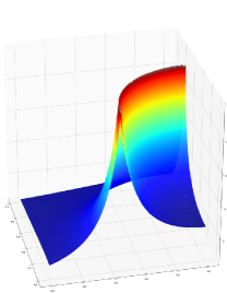
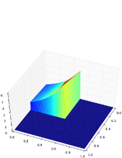
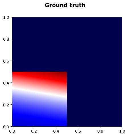
The Jakeman test functions We exercise our model on two synthetic datasets from Jakeman und Roberts (2011), both defined on the unit square. The Jakeman1 function, Figure 4,

$$f_{1}(x_{1},x_{2})=\frac{1}{|0.3-x_{1}^{2}-x_{2}^{2}|+0.1}$$ (23)

is discontinuous at $x_{1}^{2}+x_{2}^{2}=0.3$, and the Jakeman4 function, Figure 6,

$$f_{4}(x_{1},x_{2})=\begin{cases}0&\text{ if }x_{1}>0.5\text{ or }x_{2}>0.5\\ \exp(0.5x_{1}+3x_{2})&\text{otherwise}\end{cases}$$ (24)

exhibits a jump at $x_{1}=0.5,x_{2}\in[0,0.5]$ and $x_{2}=0.5,x_{1}\in[0,0.5]$.

To make things interesting, i.i.d. Gaussian noise is added to the training samples. XGBoost can cope with the noise through subsampling: Only a random fraction of the training samples pass down a tree. We observed that subsampling plays a key role when the function exhibits a discontinuity, otherwise its benefit is minor if the function has a jump. For subsampling to be effective, a large number of trees must be built. Hence subsampling degrades the performance of LinXGBoost. It is better to increase the minimum number of samples at a leaf: The linear fit to the underlying function is more robust (less susceptible to be altered by the noise) if we consider more samples. A positive side-effect is that the trees are shallower and thus the compute gets faster.

Table 1: NMSE results on the Jakeman synthetic test datasets. Smaller values are better.

	Jakeman1	Jakeman1	Jakeman4	Jakeman4
Method	11-x-11	41-x-41	11-x-11	41-x-41
XGBoost	0.0858 $\pm$ 0.0026	0.0083 $\pm$ 0.0002	0.5778 $\pm$ 0.0214	0.1335 $\pm$ 0.0021
LinXGBoost	0.0724 $\pm$ 0.0094	0.0046 $\pm$ 0.0004	0.6480 $\pm$ 0.0294	0.1385 $\pm$ 0.0024
Random Forest	0.0838 $\pm$ 0.0020	0.0113 $\pm$ 0.0002	0.5907 $\pm$ 0.0194	0.1376 $\pm$ 0.0022

Datasets are gridded: Training is carried out on the small 11-x-11 and medium 41-x-41 configurations, and testing is done on a 1001-x-1001 configuration. All model parameters are tuned for each run of an experiment by conducting an exhaustive grid search (10-fold cross-validation on the training data set). An experiment consists of 20 runs. The number of LinXGBoost trees is fixed, whereas the best number of XGBoost trees is found by cross-validation. The XGBoost regularizer $\lambda$ was set to 0, the best setting in all circumstances. Results are presented in table 1.

(a) 3D view.

(b) Projection onto the XY-plane.

Figure 3: The Jakeman1 test function.

(a) Training dataset: 11-x-11 noisy samples

(b) Training dataset: 41-x-41 noisy samples

Figure 4: Results for the noisy Jakeman1 test function ($\sigma^{2}=0.05$) for a random run (see eq. 23). Training sample data is gridded. Next to the contours, we plot the results on the diagonal $x_{1}=x_{2}$.

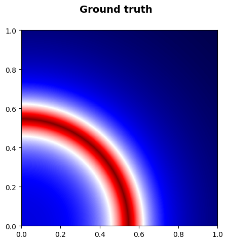
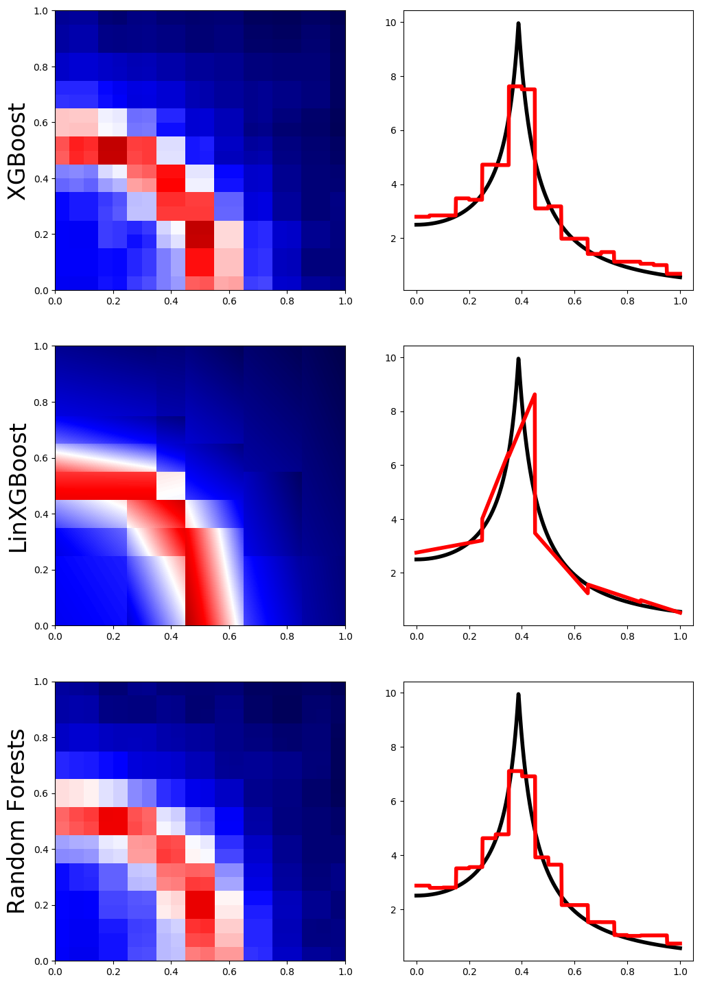
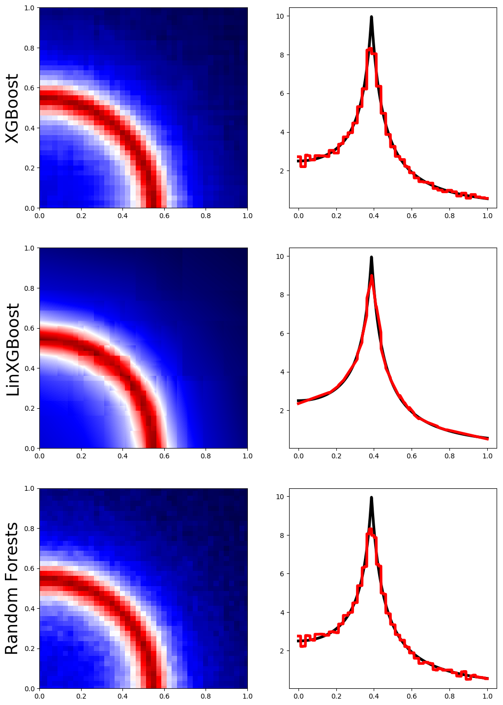
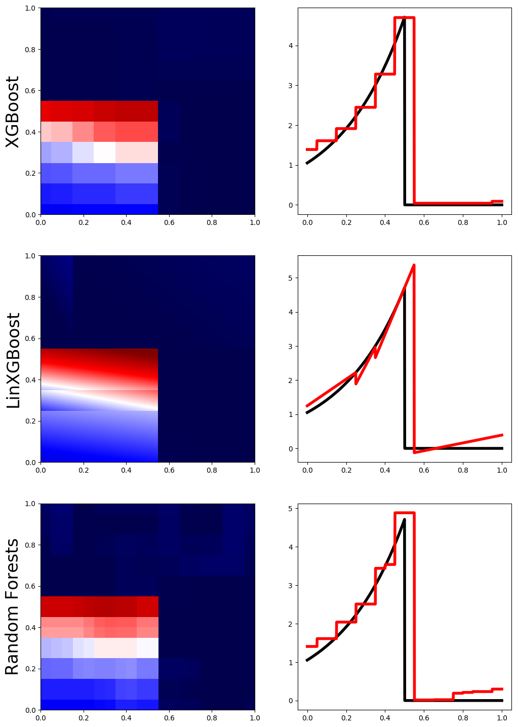
For the Jakeman1 function, on the small training dataset, LinXGBoost has 3 trees whereas XGBoost has around 50 trees (the exact number is run-dependent). There is no clear-cut winner but we observe that the variance of LinXGBoost results is fairly high. On the medium training dataset, LinXGBoost has 5 trees and XGBoost needs circa 150 trees. Nevertheless, LinXGBoost beats XGBoost by a large margin. Random Forest performs slightly worse than XGBoost. A random run is shown in Figure 4.

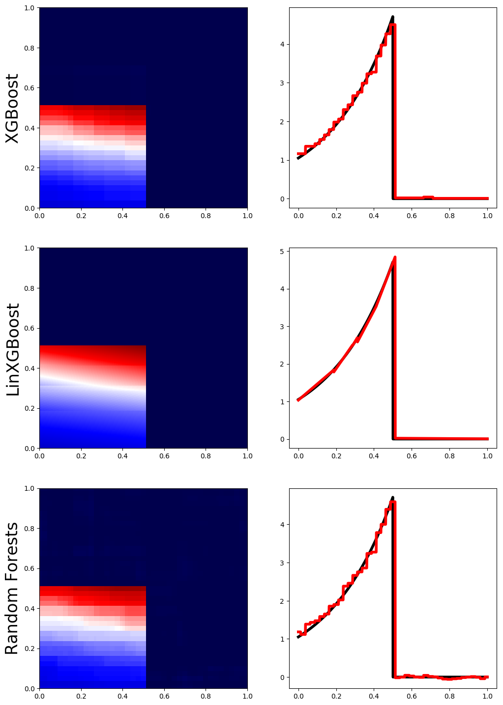
Again our expectations, LinXGBoost performs slightly worse than XGBoost and Random Forest on the Jakeman4 function on the small training dataset. Results of all methods are close to each other in terms of NMSE on the medium dataset. LinXGBoost is limited to 3 trees. Including more trees in LinXGBoost model does not improve performance. The main contribution to the error comes from the jump being at the wrong position: All methods put the jump far to the right The improvement of LinXGBoost in smoother regions is marginal though visually noticeable. Both assertions can be verified on the random run shown in Figure 6.

(a) 3D view.

(b) Projection onto the XY-plane.

Figure 5: The Jakeman4 test function.

(a) Training dataset: 11-x-11 noisy samples

(b) Training dataset: 41-x-41 noisy samples

Figure 6: Results for the noisy Jakeman4 test function ($\sigma^{2}=0.05$) for a random run (see eq. 24) . Training sample data is gridded. Next to the contours, we plot the results on the line $x_{1}=0.1$.

The Friedman1 test function The Friedman1 data set is a synthetic dataset. It has been previously employed in evaluations of MARS, Friedman (1991), and bagging, Breiman (1996). According to Friedman, it is particularly suited to examine the ability of methods to uncover interaction effects that are present in the data. In its basic version, there are 10 independent covariates, uniformly distributed on (0,1) and only five of these are related to the target via

$$y=10\sin(\pi x_{1}x_{2})+20(x_{3}-0.5)^{2}+10x_{4}+5x_{5}+\epsilon$$ (25)

where $\epsilon$ is Gaussian noise with $\sigma=1$.

We consider the dataset from the LIACC repository that contains 40768 data points. Results are averaged over 20 randomly splits of this data set. Each split has 200 training and 40568 testing points. Model parameters are tuned for each split by a 10-fold cross-validation on the training data set.

In a random run, we found that LinXGBoost needs 2 to 3 trees and so for the experiment the number of trees in LinXGBoost is either 2 or 3 (determined by cross-validation), whereas XGBoost has approximately 50 estimators. Results are presented in table 2. The error of Random Forest is twice as high as the error of XGBoost, and LinXGBoost does even better than XGBoost on average, but LinXGBoost results are a bit more volatile, presumably because LinXGBoost uses very few trees.

Table 2: NMSE results on the Friedman1 synthetic test dataset. Smaller values are better.

Method	Friedman1
XGBoost	0.1303 $\pm$ 0.0138
LinXGBoost	0.1133 $\pm$ 0.0199
Random Forest	0.2278 $\pm$ 0.0197

The Combined Cycle Power Plant Data Set (CCPP) The dataset, available at the UCI Machine Learning Repository, contains 9568 data points collected from a Combined Cycle Power Plant over 6 years (2006-2011), when the power plant was set to work with full load. Features consist of hourly average ambient variables Temperature (T), Ambient Pressure (AP), Relative Humidity (RH) and exhaust Vacuum (V) to predict the net hourly electrical energy output (PE) of the plant.

Among all datasets used for the benchmark, this dataset is the only real-world dataset that was not purposely generated for the validation of algorithms. As such, we cannot rule out the presence of outliers. Outliers have a detrimental impact on the results of XGBoost and LinXGBoost because both make use of the square loss function. Nevertheless, this impact is attenuated by the fact that XGBoost and LinXGBoost are based on decision trees and so outliers are isolated into small clusters. Extreme values do not affect the entire model because of local model fitting.

The summary of the data set per variable is:

                AT            V           AP           RH           PE
count  9568.000000  9568.000000  9568.000000  9568.000000  9568.000000
mean     19.651231    54.305804  1013.259078    73.308978   454.365009
std       7.452473    12.707893     5.938784    14.600269    17.066995
min       1.810000    25.360000   992.890000    25.560000   420.260000
25%      13.510000    41.740000  1009.100000    63.327500   439.750000
50%      20.345000    52.080000  1012.940000    74.975000   451.550000
75%      25.720000    66.540000  1017.260000    84.830000   468.430000
max      37.110000    81.560000  1033.300000   100.160000   495.760000

All features are real-valued (no categorical features). Furthermore, there are no missing values.

Are there extreme outliers ? Any point beyond 2*step where step=1.5(Q3-Q1) is considered an extreme outlier, whereas a point beyond a step is considered a mild outlier . Recall that Q1 and Q3 are the 25th and 75th percentile of the data for a given variable respectively. Answer: No.

Are there multivariate outliers ? A scatter-plot matrix is an appropriate tool to rapidly scrutinize many variables for patters (for linear trends, the correlation coefficients are printed) and outliers. Figure 7 clearly reveals some abnormalities:

• There are 13 points at the lower end of variable V (colored red) that are away from the bulk of points (colored blue): 7 points for which V=25.36 and 6 points for which V=25.88.

• There are 2 isolated points (colored red) at the lower end of variable PE.

• There is a strip of 15 points (colored green) for which V=71.14, which indicates that the data is likely to have been thresholded.

All those points can all the more safely be removed from the data set since we have plenty of data points.

Figure 7: Scatter-plot matrix for the CCPP dataset. Points that are not colored blue are considered outliers.

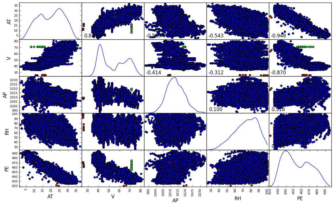
Another key property of the data set depicted in Figure 7 is that the target PE seems to be a (highly noisy) linear function of variable AT: The coefficient of correlation tops at -0.95. Hence a linear regression is a worthy contender to XGBoost, LinXGBoost and Random Forest for this particular problem.

The 9568 records set is split into training and test sets in a 70-30 proportion. The split is repeated 20 times independently. For each split, a 3-fold cross-validation is carried out to find the best hyperparameters.

Results are presented in table 3. XGBoost wins by a large margin and Random Forest performs slightly better than LinXGBoost with 4 trees. Results from the linear regression are fairly good and define the base line, but it is no surprise since the relationship between target and features is almost linear.

Pumadyn-8nm The data set was generated using a robot-arm simulation. It is highly non-linear and has very low noise. It contains 8192 data samples with 8 attributes. We follow exactly the same procedure as with the CCPP data set. Table 3 shows that XGBoost with 150 estimators (set variable) provides slightly better results than Random Forest with 100 estimators (also set variable) and LinXGBoost with 3 estimators.

Table 3: NMSE results on the CCPP (Combined Cycle Power Plant) and pumadyn-8nm datasets. Smaller values are better.

Method	CCPP	pumadyn-8nm
Linear reg.	0.07133 $\pm$ 0.00283	0.48262 $\pm$ 0.01152
XGBoost	0.03371 $\pm$ 0.00233	0.03737 $\pm$ 0.00145
LinXGBoost	0.03567 $\pm$ 0.00289	0.03876 $\pm$ 0.00177
Random Forest	0.03988 $\pm$ 0.00260	0.03898 $\pm$ 0.00138

5 Conclusion

The gradient boosting algorithm XGBoost was extended into LinXGBoost so that linear models are stored at the leaves. Computations are still analytically tractable.

This strategy is supposed to rip benefits in terms of accuracy in low dimensional input space but it is computationally intensive. As expected, experiments demonstrate that far fewer trees (in general less than five) are needed to get the accuracy XGBoost yields with hundreds of trees. LinXGBoost seems to shine in one-dimensional problems, but in higher input dimensions, it does not clearly beat XGBoost or Random Forest.

In a future work, we will investigate whether LinXGBoost can offer substantial improvements in classification.

Code

The LinXGBoost code is written in Python. It is not an extension of XGBoost. Why ? At the first sight, the XGBoost code can appear arcane because of precisely what makes XGBoost awesome: It is written in C++ and ported to R, Python, Java, Scala, and more, it runs on a single machine, Hadoop, Spark, Flink and DataFlow, and it is highly optimized. All of this bloats the code and makes it harder to pinpoint the core routines to change (and to apply the changes without breaking any feature of XGBoost!). We felt it is far more easier to implement LinXGBoost from scratch. LinXGBoost is a naive implementation in Python in less than 350 human-readable lines based on Chen (2014). Hence the interpretation of the parameters is obvious: It complies with Chen (2014).

The LinXGBoost implementation does not strive for speed. The current version runs only on a single machine and is not multithreaded. Therefore, we do not mention runtime performance.

The software implementation is made available at https://github.com/ldv1. It is envisaged to extend the XGBoost code in a future work.

References

- Adams und MacKay (2007) \NAT@biblabelnumAdams und MacKay 2007 Adams, Ryan P. ; MacKay, David J.: Bayesian online changepoint detection. In: arXiv preprint arXiv:0710.3742 (2007)
- Breiman (1996) \NAT@biblabelnumBreiman 1996 Breiman, Leo: Bagging predictors. In: Machine learning 24 (1996), Nr. 2, S. 123–140
- Chen (2014) \NAT@biblabelnumChen 2014 Chen, Tianqi: Introduction to boosted trees. In: October. https://homes. cs. washington. edu/~ tqchen (2014)
- Chen und Guestrin (2016) \NAT@biblabelnumChen und Guestrin 2016 Chen, Tianqi ; Guestrin, Carlos: XGBoost: A Scalable Tree Boosting System. In: CoRR abs/1603.02754 (2016). – URL http://arxiv.org/abs/1603.02754
- Donoho und Johnstone (1995) \NAT@biblabelnumDonoho und Johnstone 1995 Donoho, David L. ; Johnstone, Iain M.: Adapting to unknown smoothness via wavelet shrinkage. In: Journal of the american statistical association 90 (1995), Nr. 432, S. 1200–1224
- Elith u. a. (2008) \NAT@biblabelnumElith u. a. 2008 Elith, Jane ; Leathwick, John R. ; Hastie, Trevor: A working guide to boosted regression trees. In: Journal of Animal Ecology 77 (2008), Nr. 4, S. 802–813
- Englert (2012) \NAT@biblabelnumEnglert 2012 Englert, Peter: Locally Weighted Learning. In: Seminar Class on Autonomous Systems, 2012
- Friedman u. a. (2001) \NAT@biblabelnumFriedman u. a. 2001 Friedman, Jerome ; Hastie, Trevor ; Tibshirani, Robert: The elements of statistical learning. Bd. 1. Springer series in statistics New York, 2001
- Friedman (1991) \NAT@biblabelnumFriedman 1991 Friedman, Jerome H.: Multivariate adaptive regression splines. In: The annals of statistics (1991), S. 1–67
- Jakeman und Roberts (2011) \NAT@biblabelnumJakeman und Roberts 2011 Jakeman, J. D. ; Roberts, S. G.: Local and Dimension Adaptive Sparse Grid Interpolation and Quadrature. In: ArXiv e-prints (2011), September
- Kim u. a. (2005) \NAT@biblabelnumKim u. a. 2005 Kim, Hyoung-Moon ; Mallick, Bani K. ; Holmes, CC: Analyzing nonstationary spatial data using piecewise Gaussian processes. In: Journal of the American Statistical Association 100 (2005), Nr. 470, S. 653–668
- Lee (2002) \NAT@biblabelnumLee 2002 Lee, Thomas C.: Automatic smoothing for discontinuous regression functions. In: Statistica Sinica (2002), S. 823–842
- Meier u. a. (2014) \NAT@biblabelnumMeier u. a. 2014 Meier, Franziska ; Hennig, Philipp ; Schaal, Stefan: Local Gaussian Regression. In: arXiv preprint arXiv:1402.0645 (2014)
- Park und Huang (2016) \NAT@biblabelnumPark und Huang 2016 Park, Chiwoo ; Huang, Jianhua Z.: Efficient Computation of Gaussian Process Regression for Large Spatial Data Sets by Patching Local Gaussian Processes. In: Journal of Machine Learning Research 17 (2016), Nr. 174, S. 1–29. – URL http://jmlr.org/papers/v17/15-327.html
- Park u. a. (2011) \NAT@biblabelnumPark u. a. 2011 Park, Chiwoo ; Huang, Jianhua Z. ; Ding, Yu: Domain decomposition approach for fast Gaussian process regression of large spatial data sets. In: Journal of Machine Learning Research 12 (2011), Nr. May, S. 1697–1728
- Plagemann u. a. (2008) \NAT@biblabelnumPlagemann u. a. 2008 Plagemann, Christian ; Kersting, Kristian ; Burgard, Wolfram: Nonstationary Gaussian process regression using point estimates of local smoothness. In: Machine learning and knowledge discovery in databases (2008), S. 204–219
- Rasmussen und Ghahramani (2002) \NAT@biblabelnumRasmussen und Ghahramani 2002 Rasmussen, Carl E. ; Ghahramani, Zoubin: Infinite mixtures of Gaussian process experts. In: Advances in neural information processing systems 2 (2002), S. 881–888
- Torgo (1997) \NAT@biblabelnumTorgo 1997 Torgo, Luís: Functional models for regression tree leaves. In: ICML Bd. 97, 1997, S. 385–393