Differential-activity driven instabilities in biphasic active matter

Abstract

Active stresses can cause instabilities in contractile gels and living tissues. Here we describe a generic hydrodynamic theory that treats these systems as a mixture of two phases of varying activity and different mechanical properties. We find that differential activity between the phases provides a mechanism causing a demixing instability. We follow the nonlinear evolution of the instability and characterize a phase diagram of the resulting patterns. Our study complements other instability mechanisms in mixtures such as differential growth, shape, motion or adhesion.

Biological systems are distinguished by the presence of active stresses which can affect their physical properties and alter their stability. For example, active stresses give rise to collectively moving streaks Schaller and clusters Dombrowski_2004 ; pnas_bacteria ; VibratedDisks2013 , rotating ring, swirl or aster-like patterns Backouche_phase_diagram_active_gels ; Kudrolli_2008 ; Yutaka ; Ringe_PNAS ; mori2011intracellular ; Needleman_microtubule_contraction , or the remodelling of cell-to-cell junctions in living tissues rauzi2010planar . These systems are typically described as a single phase with active stresses that drive the assembly of the constituents and the properties of the phases are typically assumed as liquid-like bois2011pattern ; Toner_2012 ; prost2015active or even gases Aronson_MT ; Bertin_long ; Weber_NJP_2013 ; thuroff2013critical .

However many active material cannot be treated as fluids. Examples include cartilage, bone, tissues in early development Barna2007931 ; Tabler20164 ; Martinjcb.200910099 , and superprecipitated systems such as networks of filaments connected by crosslinks and molecular motors mori2011intracellular ; Bendix20083126 ; Needleman_microtubule_contraction . The presence of activity in these systems can drive the macroscopic contraction of gels (mori2011intracellular ; Bendix20083126 ; Needleman_microtubule_contraction , and Fig. 1(a,b)), the compaction of cells during the condensation of cartilage cells Barna2007931 , the network formation of osteoblasts during skull closure in embryos Tabler20164 , and the formation of furrows in tissues Martinjcb.200910099 . This requires the augmentation of previous passive biphasic descriptions, such as associated with poroelasticity maha_cytoplasm_poroelastic_material to account for active stress regulation and diffusion in cells and tissues. While recent work has included activity in a poroelastic description radszuweit2013intracellular ; radszuweit2014active , the material was assumed to be homogeneous and stable despite active stress generation in one of the phases. Here we question this assumption of stability of an active mixture composed of two phases with different mechanical properties, and ask under what physical conditions an active poroelastic material might contract/condense or disintegrate/fragment, a phenomenon seen in a variety of experimental systems (Fig. 1(a-c)).

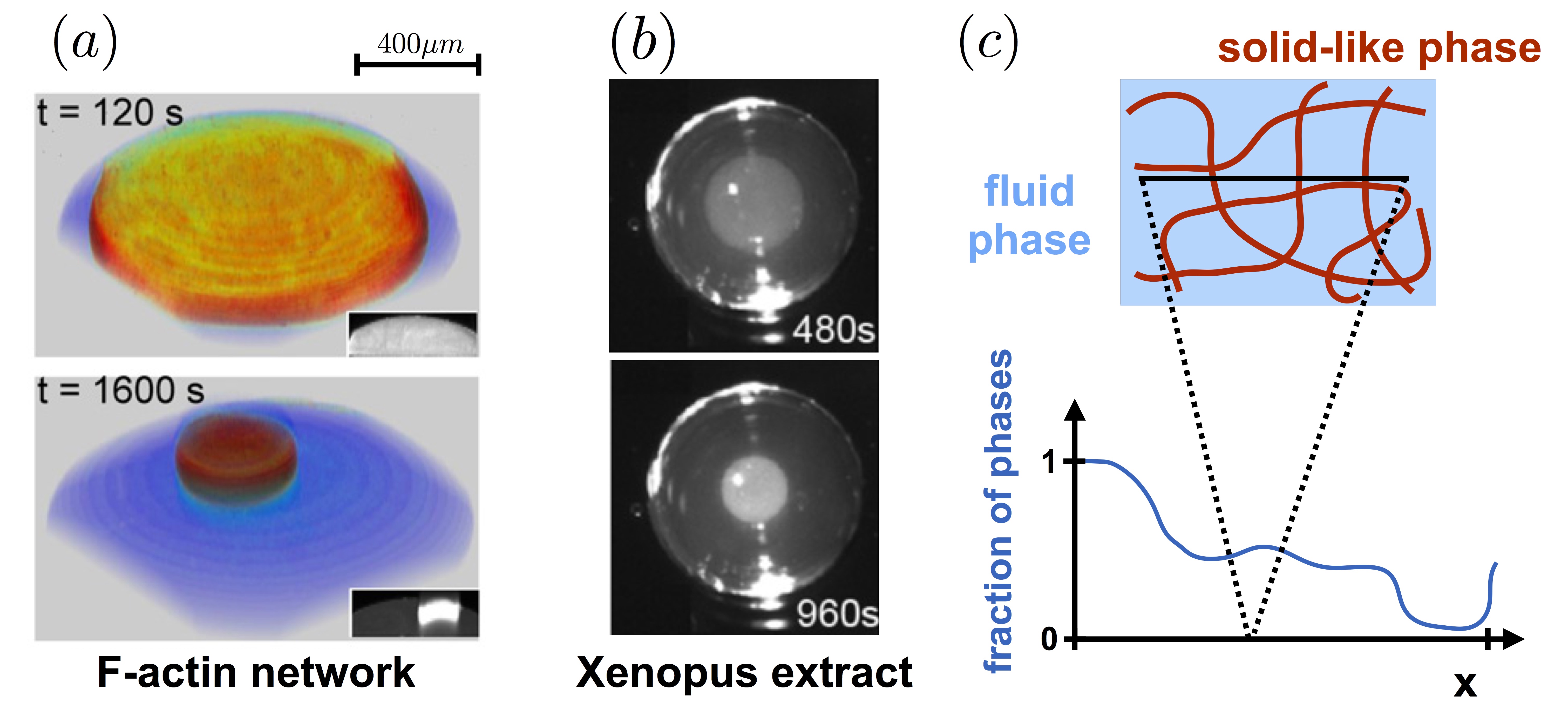
Figure 1: Examples of unstable, biphasic mixtures and illustration of two-phase mixture theory. (a) Contractile behavior of actin-myosin II network crosslinked with $\alpha$-actinin, and (b) contracting Xenopus egg extract; both are taken from Ref. Bendix20083126 . (c) Illustration of biphasic mixture theory. Microscopic illustration of a biphasic gel (top), and hydrodynamic representation on large wavelength described by the volume fraction field of the constituent phases (bottom). The theory is valid on length scales above the pore size. On these scales, hydrodynamic variables are continuous, impact of microscopic interfaces is captured as friction proportional to the velocity difference skotheim2004dynamics , and the isotropic part of the activity should dominate any anisotropic contribution since activity is typically generated on or below the scale of the pore.

We find that differential activity between the solid and fluid phases that constitute an initially homogeneneous poroelastic medium can drive a mechanical instability leading to the demixing of a homogeneous medium into condensed solid-like patches that arise due to macroscopic contraction, reminiscent of observations in superprecipitated gels and compacted cells in tissues. Depending on the rate and ability of transport of material and stress in the biphasic material, we find both uniformly growing and pulsatile instabilities leading to assembling, disassembling and drifting solid-like clusters that undergo fusion and fission.

We start with a consideration of isotropic active systems composed of two immiscible phases, $i=1,2$. These systems can be described by a hydrodynamic theory similar to descriptions used for fluid-like biphasic matter drew1983mathematical ; keener2011kinetics , or elastic doi_review_swelling_and_volume_PT and viscoelastic gels tanaka1993unusual ; tanaka2000viscoelastic . This theory is valid on length scales above the characteristic pore size of the solid-like phase (Fig. 1(c)). At the simplest level, activity in our biphasic system is described as an isotropic active stress that acts on each phase which responds to this stress according to its passive mechanical properties which are either fluid or solid-like, respectively. Each phase $(i)$ is described by the hydrodynamic variables of velocity $v^{(i)}_{\alpha}$, volume fraction $\phi^{(i)}$ and displacement $u^{(i)}_{\alpha}$ with $\partial_{t}u^{(i)}_{\alpha}=v^{(i)}_{\alpha}$. The overall system is assumed to be incompressible and fully occupied by the two phases, i.e. $\phi\equiv\phi^{(1)}=1-\phi^{(2)}$. The fractions of each phase $i$ are conserved, so that $\partial_{t}\phi^{(i)}=-\partial_{\alpha}(\phi^{(i)}v^{(i)}_{\alpha}+j^{(i)}_{\alpha})$, where $j^{(i)}_{\alpha}$ denotes a relative flux between the phases with $j^{(1)}_{\alpha}=-j^{(2)}_{\alpha}=:j_{\alpha}$. This relative flux can for example stem from rare unbinding events of components that belong to one of the phases. The resulting unbound components can diffuse and thereby cause an effective diffusive flux of the bound components (see Supplemental Material SM , I). For simplicity, we write $j_{\alpha}=-D\partial_{\alpha}\phi$, where $D$ denotes the diffusion constant. The two conservation laws can be equivalently expressed by one transport equation and an incompressibility condition,

$$\partial_{t}\phi =-\partial_{\alpha}\left(\phi v^{(1)}_{\alpha}\right)+D\partial_{\alpha}^{2}\phi\,,$$ (1a)

$$0 =\partial_{\alpha}\left[\phi\,v^{(1)}_{\alpha}+\left(1-\phi\right)v^{(2)}_{\alpha}\right]\,.$$ (1b)

Neglecting osmotic effects and inertia, force balance in each phase implies:

$$0 =\partial_{\beta}\left(\phi\sigma_{\alpha\beta}^{(1)}\right)-\phi\partial_{\alpha}p-\mathcal{F}_{\alpha}\,,$$ (2a)

$$0 =\partial_{\beta}\left((1-\phi)\sigma_{\alpha\beta}^{(2)}\right)-(1-\phi)\partial_{\alpha}p+\mathcal{F}_{\alpha}\,,$$ (2b)

where $$\sigma_{\alpha\beta}^{(i)} p \mathcal{F} \mathcal{F} \mathcal{F}_{\alpha}=\Gamma(\phi)(v^{(1)}_{\alpha}-v^{(2)}_{\alpha}) \Gamma(\phi)=\Gamma_{0}\phi(1-\phi) \Gamma_{0} \mathcal{F}=0 \phi=0 \phi=1 \sigma_{\alpha\beta}^{(i),\text{p}} {A}^{(i)}$$ is the additional stress (beyond the pressure) in each phase, and we have assumed, as in mixture theory barry2001asymptotic ; cowin2012mixture ; skotheim2004dynamics that this stress is weighted by the respective volume fraction footnote2 . The pressure acts as a Lagrange multiplier that ensures the incompressibility condition Eq. (S10b). Momentum transfer between the phases is described by a friction force density . To leading order is proportional to the relative velocity of the phases, , where is the friction coefficient between the phases with constant. The dependence of the friction coefficient on volume fraction is a consequence of the condition that hydrodynamic momentum transfer vanishes if one of the phases is absent, i.e.  for or . Finally, we additively decompose the stress into the passive stress and the isotropic activity ,

$$\sigma_{\alpha\beta}^{(i)} =\sigma_{\alpha\beta}^{(i),\text{p}}+{A}^{(i)}\,\delta_{\alpha\beta}\,,$$ (2c)

where the passive stress $\sigma_{\alpha\beta}^{(i),\text{p}}$ characterizes the mechanical properties of each phase. In general, the activity depends on all hydrodynamic variables. For simplicity, we focus on activities that depend on the volume fraction $\phi$, ${A}^{(i)}={A}^{(i)}(\phi)$. Eqs. (2) can be rewritten as

$$0 =\partial_{\beta}\left(\phi\sigma_{\alpha\beta}^{(1)}+(1-\phi)\sigma_{\alpha\beta}^{(2)}-\delta_{\alpha\beta}p\right)\,,$$ (3a)

$$0 =\partial_{\beta}\left(\phi\,\sigma^{(1),\text{p}}_{\alpha\beta}\right)-\frac{\phi}{1-\phi}\partial_{\beta}\left((1-\phi)\sigma^{(2),\text{p}}_{\alpha\beta}\right)$$

$$+\left(v^{(2)}_{\alpha}-v^{(1)}_{\alpha}\right)\Gamma_{0}\phi+\phi\,{{A}}(\phi)\partial_{\alpha}\phi\,,$$ (3b)

where we define

$${{A}}(\phi)=\left[\frac{{A}^{(1)}}{\phi}+\frac{{A}^{(2)}}{1-\phi}+\frac{\text{d}}{\text{d}\phi}\left({A}^{(1)}-{A}^{(2)}\right)\right]\,$$ (3c)

as the differential activity. The derivatives of the activity ${A}^{(i)}$ with respect to $\phi$ appear because gradients of stress enter the force balance Eqs. (S10a) and (S10e), while the dependencies on the activity ${A}^{(i)}$ are a consequence of treating the system as a biphasic mixture, i.e. weighting the stress contributions by the respective volume fractions; see Supplemental Material SM , II for more details on Eq. (S7). The specific form of the activities ${A}^{(i)}$ depends on the system of interest.

As our first example, we consider a one dimensional, biphasic mixture composed of a (Kelvin) viscoelastic solid, (s), and a fluid phase, (f), with the constitutive equations:

$$\sigma^{\text{s},\text{p}} =\lambda\partial_{x}u+\zeta\partial_{x}v\,,$$ (4a)

$$\sigma^{\text{f},\text{p}} =0\,,$$ (4b)

where the one dimensional solid displacement and velocity are $u$ and $v=\text{d}u/\text{d}t\equiv\dot{u}$; the fluid velocity is given by $-v\phi/\left(1-\phi\right)$. In eq. (4a), $\lambda$ denotes the Lamé coefficient and $\zeta$ is the bulk solid viscosity. The viscous stress in the fluid phase can be approximated to zero since fluid strains are negligible relative to solid strains on length scales above the pore size, and in the systems of interest, the solid viscosity typically exceeds the fluid viscosity by several orders in magnitude spiegelman1987simple . Since diffusive transport of constituents in this solid-fluid mixture is expected to be slow compared to solid momentum transport, we consider the limit of small diffusivities and use rescalings of length and time scales not containing the diffusion constant. Specifically, we rescale time and length as $t\to(\zeta/\lambda)\,t$ and $x\to\ell\,x$ with $\ell=\sqrt{\zeta/\Gamma_{0}}$, so that velocities $v\to v\,\ell\lambda/\zeta$ and the scaled equations read:

$$\partial_{t}\phi =-\partial_{x}(\phi\dot{u})+\tilde{D}\partial_{x}^{2}\phi\,,$$ (5a)

$$0 =\partial_{x}\left(\phi\partial_{x}u+\phi\partial_{x}v\right)+\phi\tilde{A}(\phi)\,\partial_{x}\phi-\frac{\phi}{1-\phi}\dot{u}\,.$$ (5b)

There are two dimensionless parameters in Eqs. (5), measuring the strength of differential activity, $\tilde{A}={{A}}/\lambda$ and diffusivity, $\tilde{D}=D\Gamma_{0}/\lambda$.

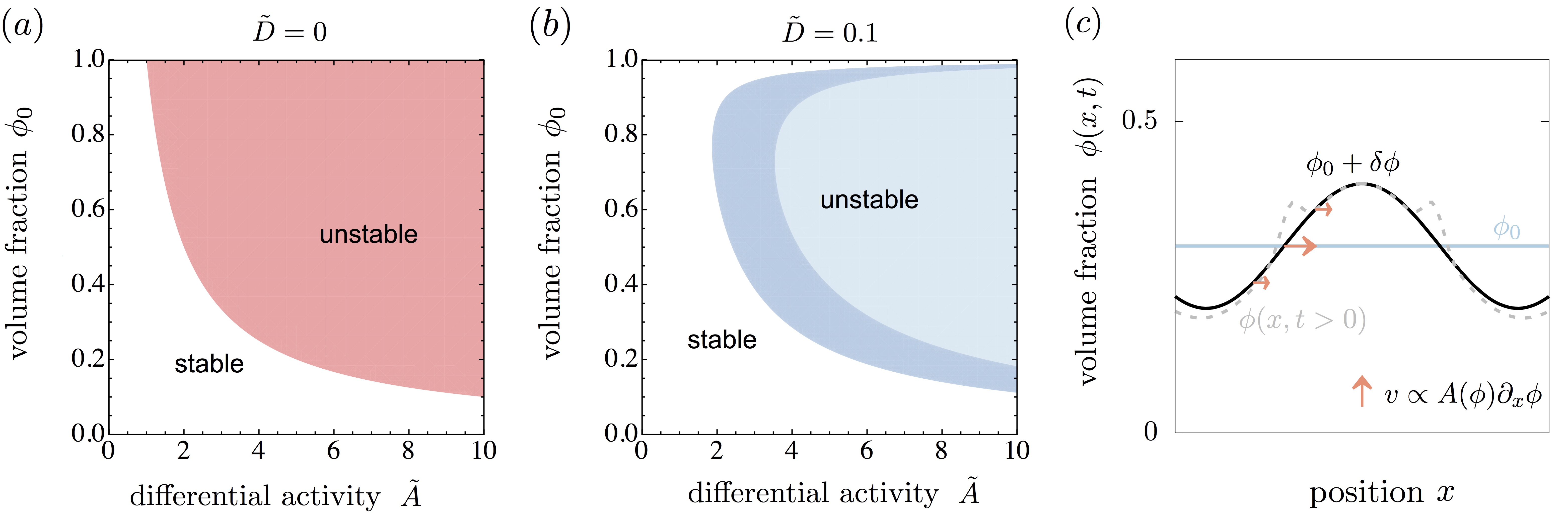
Figure 2: (a,b) Stability diagrams as a function of volume fraction $\phi$ and non-dimensional differential activity $\tilde{A}$ obtained from the linear stability analysis of Eqs. (3). The diagram indicate the parameter regimes where the homogeneous base state is stable or unstable. Diagrams with constant $\tilde{A}$ and for diffusivities (a) $\tilde{D}=0$ and (b) $\tilde{D}=0.1$. The colored regions depict $\Re(\omega_{+})>0$. Red indicates an instability where $\Im(\omega_{k})=0$, while for dark/light blue corresponds to $\Im(\omega_{k})\not=0$ for all $q$/or for a finite waveband. (c) Illustration of the instability mechanism driven by differential activity ${A}(\phi)$. Small perturbations in volume fraction, $\phi_{0}\to\phi_{0}+\delta\phi$, are amplified since differential activity causes a drift velocity that points toward the maximum of a local inhomogeneity of volume fraction. To lowest order in $q$, this velocity (red horizontal arrows) scales as $v\propto{{A}}\partial_{x}\phi$ (Eq. (5b)), further increasing the initial perturbation. Because the velocity decreases to zero close to the extrema of the perturbation ($\partial_{x}\phi=0$), spike may emergence (gray dashed line, $\phi(x,t>0)$), which can move inward by diffusion and thereby further amplify the instability.

To understand the stability of a homogenous base state given by $u=u_{0}$, $\dot{u}=0$ and $\phi=\phi_{0}$, we perturb the volume fraction of the phases and the displacement and expand the perturbation in terms of Fourier modes of the form $\propto\text{e}^{\omega t+iqx}$ and linearize the equations above. Calculating the largest growing mode to linear order in diffusivity $\tilde{D}$ and to the fourth order in the wavenumber $q$ gives

$$\Re(\omega_{+}) \simeq\frac{q^{2}}{B}\left[-1+\tilde{A}\phi_{0}\left(1-\frac{\tilde{D}\,B}{\tilde{A}\phi_{0}-1}\right)\right]$$ (6)

$$-\frac{q^{4}}{B^{2}}\left(\tilde{A}\phi_{0}-1\right)\,,$$

for $\phi_{0}\in[0,1]$ and $\tilde{A}\phi_{0}>1$, and where $B=1/(1-\phi_{0})$. We see that there is a long wave length instability with $\Re[\omega_{+}(q)]>0$ leading to growth of the homogeneous state. The instability is driven by differential activity ${A}$ which competes with frictional momentum transfer between the phases, and diffusion of displacement, velocity and volume fraction. At the onset of the instability where spatial inhomogeneities in strain are negligible, long wavelength perturbations in volume fraction are amplified because differential activity causes a solid drift velocity $\dot{u}$ that points toward the maximum of a local inhomogeneity of volume fraction (Fig. 2(c)). This drift scales as $\dot{u}\propto\tilde{A}\partial_{x}\phi$ to lowest order in $q$ (Eq. (5b). If ${A}>0$, the velocity is parallel to the gradient in solid fraction and thus leads a local increase in the solid volume fraction. The velocity at onset of the instability is zero at the local maximum of the inhomogeneity ($\partial_{x}\phi=0$). This causes the emergence of spikes in the volume fraction around the initial inhomogeneity where $\partial_{x}\phi$ is largest. These spikes can move inward due to diffusion and amplify the initial perturbation (see movies in Supplemental Material SM ,V).

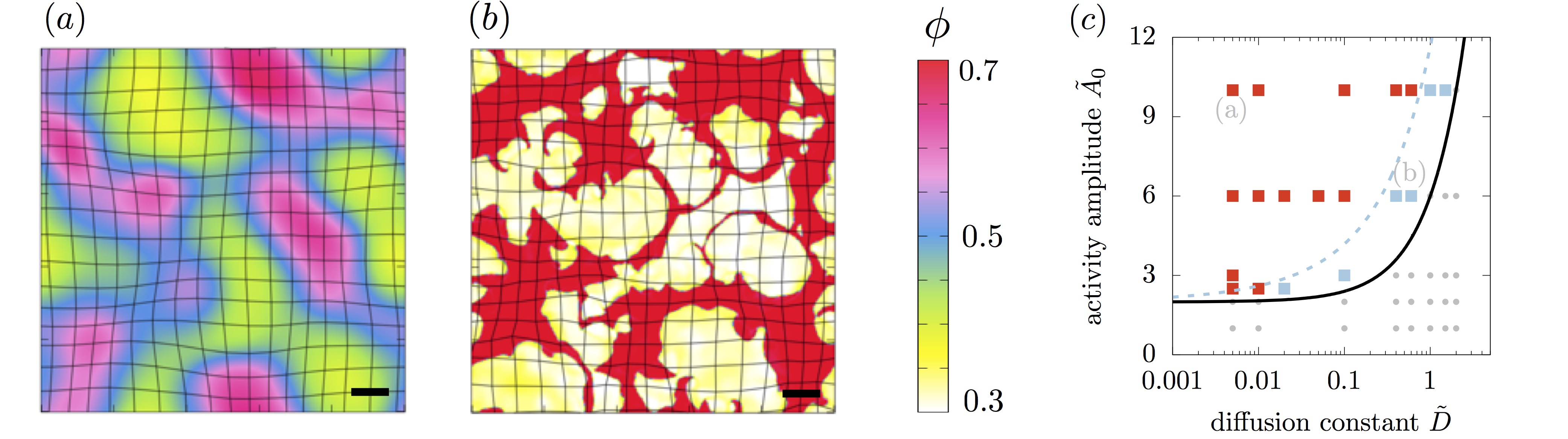
Figure 3: Patterns and phase diagram in two dimensions obtained from numerically solving Eqs. (3) (see Supplemental Material SM , IV,V for details). (a,b) Two representative snapshots of patterns observed in our active poroelastic model. Black bar depicts the unit length $\ell=\sqrt{\zeta/\Gamma_{0}}$. Parameters: $\phi_{0}=0.5$, and (a) $\tilde{D}=0.4$ and $\tilde{A}_{0}=6$, (b) $\tilde{D}=0.005$, $\tilde{A}_{0}=10$. The black lines depict the displacements of the solid phase. (c) Phase diagram as a function of non-dimensional diffusivity $\tilde{D}$ and activity amplitude $A_{0}$. Squares indicate parameters where the numerical solution shows the emergence a spatial-temporal pattern. Blue/red squares correspond to pattern morphologies reminiscent of (a)/(b). The black lines depict the result from the linear stability analysis for Poisson ratio $\nu\approx 0.5$. Parameters above the black line are linearly unstable. The parameters between the black and blue dashed lines correspond to oscillatory modes for all unstable wavenumbers. In the numerics we considered a specific choice of the activity function (Supplemental Material SM , II) to confine the range of volume fraction $\phi$ (color bar). This choice ensures the approximate validity of linear elasticity.

When the diffusivity vanishes, i.e. $\tilde{D}=0$, the instability occurs for $\tilde{A}>\tilde{A}_{c}$ with $\tilde{A}_{c}=1/\phi_{0}$ denoting the critical activity (in real units: $A_{c}=\lambda/\phi_{0}$). It is asymmetric with respect to volume fraction and the instability vanishes for $\phi_{0}\to 0$ (Fig. 2(a)). The origin of this asymmetry arises from the difference in passive properties of the two phases (Eqs. (4)). Symmetry in volume fraction can for example be restored if both phases are treated as fluids, or as viscoelastic material with equal transport coefficients. The growth rate of the largest growing mode, $\omega_{+}(q)$, is real for all wavenumbers if $\tilde{D}=0$ which indicates a non-oscillatory growth of modes (see Supplemental Material SM , III, for plots of $\omega_{k}(q)$).

For non-zero diffusivity, the critical activity increases (Eq. (6) and Fig. (3)(c) black line). The term $B=1/(1-\phi_{0})$ connected to viscous transport causes the instability to vanish also at large volume fraction (Fig. 2(b)). In addition, for $\tilde{D}\not=0$, the growth rate $\omega_{k}(q)$ can have a non-zero imaginary part. At the transition boundary between the stable and unstable regions, the growth rate is complex for all wavenumbers (dark blue/gray in Fig. 2(b)). However, deep in the unstable regime, the growth rate becomes real for small $q$ but there remains a complex and unstable band of wavenumbers (light blue/gray in Fig. 2(b)). The width of these band of wavenumbers decreases to zero as the diffusivity approaches zero (see Supplemental Material SM , III).

These two different characteristics in the growth rate obtained from the linear stability analysis indicate that nonlinear evolution of the patterns might also differ in these regimes. To investigate the pattern dynamics we numerically solved the non-linear equations in one and two dimensions; see Supplemental Material SM , II, IV,V for definitions of the used activity functions, details on the numerics, and movies. In one dimension and the limit of zero diffusion, we find that the volume fraction and displacement steadily grow; a behavior that is consistent with a real dispersion relation. In the regime of a purely complex dispersion relation domains of high and low volume fraction exhibit a tendency to synchronously oscillate with a frequency that is roughly determined by the time to diffuse the size of a domain. On longer time-scales this oscillating state can spontaneously break the left-right symmetry and the domains collectively move in one direction reminiscent of traveling fronts found in fluid-fluid biphasic matter in the presence of osmotic forces cogan2012marginal . In contrast, in the mixed case where the dispersion relation is real and complex, the domains of high and low volume fraction separated by sharp interfaces seem to drift while they undergo fusion and break-up events. In two dimensions we observe a similar dynamics. For parameters closer to the transition line where all unstable modes are oscillatory, the system shows a pulsatory type of pattern (Fig. 3(a)). Deep in the unstable regime of the stability diagram (e.g. low $\tilde{D}$ and high activity amplitude $A_{0}$) domains with sharp and roughened interfaces drift, split and fuse (Fig. 3(b)). The onset of the instability and the two pattern morphologies determined numerically match the results obtained via linear stability (Fig. 3(c)). However, in two dimensions, we do not observed a collectively moving state.

Our theory qualitatively reproduces observations in superprecipitated active systems mori2011intracellular ; Bendix20083126 ; Needleman_microtubule_contraction . After the onset of the instability and for low diffusivities, the spatial standard deviation of displacement and volume fraction steadily increases and saturates once the system reaches its quasi stationary state. Concomitantly, the velocity decreases to zero. According to our numerical results the inter-phase diffusion destablizes segregated domains on long time-scales and causes oscillatory patterns. We suppose that diffusion in superprecipitated active gels is typically too weak to observe the oscillatory type of assembly/disassembly dynamics in the simulations.

We have shown that differential activity can serve as a mechanism defining a novel class of instabilities in physics, complementing differential size asakura1954interaction , differential shape onsager1949effects , and differential adhesion flory1942thermodynamics ; huggins42 ; steinberg1970does . The mechanism of differential activity might play an essential role in various kinds of biological systems including cell sorting processes in tissues, disintegration and macroscopic contractions in super-precipitated systems and patterns in the cellular cortex or the cytoplasm. Analogously, differential activity characterizes the physical difference between two phases leading to the destablization of the homogeneous thermodynamic state. Our theory generalizes one-component active fluid approaches (e.g. bois2011pattern ) to two phases that can segregate due to the presence of active stress radszuweit2013intracellular ; radszuweit2014active . Activity and the interactions between the phases can cause an instability leading to patches where solid or fluid matter is enriched, respectively. This instability is driven by differential activity which competes with elastic, frictional and diffusive transport processes. Though we have illustrated the instability for a specific set of constitutive equations (Eqs. (4)) the existence of the instability is generic, i.e. it can occur for any combination of passive mechanical properties of the phases.

SUPPLEMENTAL MATERIAL

Supplemental Material:
Differential-activity driven instabilities in biphasic active matter

Christoph A. Weber Chris H. Rycroft L. Mahadevan

I Origin of diffusion in biphasic matter

In our model for biphasic active matter we introduced a relative diffusive flux $j^{(1)}_{\alpha}=-j^{(2)}_{\alpha}=:j_{\alpha}$ in the transport equations of volume fraction, $\partial_{t}\phi^{(i)}=-\partial_{\alpha}\left(\phi^{(i)}v^{(i)}_{\alpha}+j^{(i)}_{\alpha}\right)$, though the velocity $v^{(i)}_{\alpha}$ already captures the movement of each phase. Below we will discuss one possible mechanism for how such a diffusive flux can emerge and that it can be written as $j_{\alpha}=-D\partial_{\alpha}\phi$, where $D$ denotes the diffusion constant.

This relative flux can for example stem from rare unbinding events of components that belong to one of the phases. Here, a bound state refers to filaments connected to other filaments by molecular motors. Molecular motors can provide linkage and exert active forces on the filament phase. Unbinding means that the constituents lose connection to other filaments due to unbinding of molecular motors and can thus diffuse freely. Suppose the components inside phase 1 can unbind with a rate $\gamma_{2}$, while binding events occur with a rate $\gamma_{1}$ and their occurrence is proportional to the fraction of unbound material and the concentration of unbound molecular motors $c_{\text{M}}$. Unbound molecular motors and unbound filaments diffuse with a diffusion constant $D_{\text{M}}$ and $D_{\text{off}}$. Assuming conservation of bound plus unbound filaments, the extended transport equations of phase 1 are

$$\partial_{t}c_{\text{M}} =D_{\text{M}}\nabla^{2}c_{\text{M}}-m\gamma_{1}\phi_{\text{off}}c_{\text{M}}+m\gamma_{2}\phi\,,$$ (S1)

$$\partial_{t}\phi_{\text{off}} =D_{\text{off}}\nabla^{2}\phi_{\text{off}}-\gamma_{1}\phi_{\text{off}}c_{\text{M}}+\gamma_{2}\phi\,,$$ (S2)

$$\partial_{t}\phi_{\text{}} =\nabla\cdot(\phi\mathbf{v}^{(1)})+\gamma_{1}\phi_{\text{off}}c_{\text{M}}-\gamma_{2}\phi\,,$$ (S3)

where $m$ is a constant factor accounting for binding of multiple motors per filament.

We will now simplify the set of equations above in the limit of rare unbinding events and fast diffusion of the unbound components, $D_{\text{off}}\gg\gamma_{2}L^{2}$, where $L$ denotes the system size. This limit ensures that $\phi_{\text{off}}(\mathbf{x})\ll\phi(\mathbf{x})$ for all positions $\mathbf{x}$. Let us assume that diffusion of molecular motors relative to diffusion of unbound filaments is fast ($D_{\text{M}}\gg D_{\text{off}}$) such that that $c_{\text{M}}(\mathbf{x})$ is constant. Then Eq. (S1) gives

$$\phi_{\text{off}}\simeq\frac{\gamma_{2}\phi}{\gamma_{1}c_{\text{M}}}\,.$$ (S4)

If diffusion of unbound components is fast enough on the time-scale during which the volume fraction $\phi$ changes, we can neglect the dynamics of $\phi_{\text{off}}$, i.e. $\partial_{t}\phi_{\text{off}}\simeq 0$, giving

$$\gamma_{1}\phi_{\text{off}}c_{\text{M}}-\gamma_{2}\phi\simeq D_{\text{off}}\nabla^{2}\phi_{\text{off}}\,.$$ (S5)

Inserting Eq. (S4) into the above equation, and substituting the terms describing the binding/unbinding events in Eq. (S3), one finds

$$\partial_{t}\phi_{\text{}}=\nabla\cdot(\phi\mathbf{v}^{(1)})+D\nabla^{2}\phi_{\text{}}\,,$$ (S6)

where the diffusion constant $D=D_{\text{off}}\gamma_{2}/(\gamma_{1}c_{\text{M}})$. In summary, the diffusion of unbound components can effectively lead to a diffusion of the bound components $\phi$ with a diffusive flux that can be written as $j_{\alpha}=-D\partial_{\alpha}\phi$.

A similar argument can be constructed for loosely connected tissues such as mesenchymal tissues. The difference is only that the bound cells are active themselves, and instead of external molecular motors one could introduce the fraction of unbound cell-to-cell connections.

II Properties and possible choices of differential activity

II.1 Properties of differential activity

Differential activity is the driver for the instability discussed in our letter. In this section we discuss some basic properties of the differential activity function,

$${{A}}(\phi)=\left[\frac{{A}^{(1)}}{\phi}+\frac{{A}^{(2)}}{1-\phi}+\frac{\text{d}}{\text{d}\phi}\left({A}^{(1)}-{A}^{(2)}\right)\right]\,.$$ (S7)

Equation (S7) implies that differential activity does not vanish for equal activities, ${A}^{(1)}={A}^{(2)}$. However, differential activity can vanish even for non-zero activity in each phase, ${A}^{(i)}\not=0$. One possibility is that activities cancel within the same phase, i.e. ${A}^{(1)}={A}_{0,1}/\phi$ and ${A}^{(2)}={A}_{0,2}/(1-\phi)$, where ${A}_{0,i}$ is some constant. The other possibility is that the activity of one phase cancels the activity of the other phase, i.e. ${A}^{(1)}=\mp{A}_{0}\phi$ and ${A}^{(2)}=\pm{A}_{0}(1-\phi)$, with ${A}_{0}$ denoting some constant.

In the main text we discuss the case of constant differential activity. The differential activity ${{A}}$ can be constant and non-zero for ${A}^{(1)}=\pm{A}_{0,1}\phi$ and ${A}^{(2)}=\pm{A}_{0,2}(1-\phi)$, or ${A}^{(1)}={A}^{(2)}={A}_{0}\phi(1-\phi)$.

II.2 Possible choices of differential activity

The shape and dependencies of the activities depend on the particular system of interest. Next to a constant differential activity one could consider an asymmetric case where phase 2 is passive (${A}^{(2)}=0$) and phase 1 is active with ${A}^{(1)}={A}_{0}\,\phi(1-\phi)$, leading to a differential activity ${{A}}={A}_{0}(2-3\phi)$ (Eq. (S7)). Here, ${A}_{0}$ characterizes the amplitude of the activity. In this case the generation of active stress vanishes in the absence of phase 1 or 2, respectively. This asymmetric case is qualitatively motivated by super-precipitated systems and tissues rauzi2010planar ; maha_cytoplasm_poroelastic_material ; mori2011intracellular ; Bendix20083126 ; Needleman_microtubule_contraction ; radszuweit2013intracellular ; radszuweit2014active , where one phase is passive (intestinal fluid) while the other phase is active (filaments, cells). Moreover, activity requires a non-zero fraction of active components (${A}^{(1)}\propto\phi$ ) while there could exit an inhibitory mechanism as the active components get crowded (${A}^{(1)}\propto-\phi^{2}$). For such an activity function linear stability suggests that an instability occurs if the activity amplitude ${A}_{0}$ is larger than the critical activity $\tilde{A}_{0,c}=\left(\phi_{0}(2-3\phi_{0})\right)^{-1}$ (for vanishing diffusivity $\tilde{D}=0$). Interestingly, the instability can occur for both, positive (expansions) and negative (contractions) activity amplitudes $\tilde{A}_{0}$ (Fig. (S1)). We tested this choice of activities in our one-dimensional numerical studies and found that the emergence of spatial-temporal patterns is consistent with the results from the linear stability analysis. However, for parameters deeply in the unstable region of the stability diagram, large local strain, $\partial_{x}u$, can build up during the pattern formation violating the small strain limit of the used Hooke’s law. Thus we considered an activity function which ensures that domains cannot exhibit porosities below $\phi_{\text{min}}$ or above $\phi_{\text{max}}$. This also restricts the system to small or moderate strains. The activities thus read

$${A}^{(1)} ={A}_{0}\left[\left(\phi-\phi_{0}\right)-a\left(\phi-\phi_{0}\right)^{3}\right]\,,$$ (S8)

$${A}^{(2)} =0\,,$$ (S9)

where ${A}_{0}$ denotes the activity amplitude (non-dimensional activity amplitude $\tilde{{A}}_{0}={A}_{0}/\lambda$). It sets the scale of the active stress, but not the fixed points where the activity ${A}^{(1)}$ vanishes to zero. The latter is determined by the parameter $a>0$. Its value restricts the dynamics within the volume fractions $\phi_{\text{min}}=\phi_{0}-1/\sqrt{a}$ and $\phi_{\text{max}}=\phi_{0}+1/\sqrt{a}$. In our letter we fix the mean volume fraction to $\phi_{0}=0.5$ and $a=20$, leading to $\phi_{\text{min}}\approx 0.276$ and $\phi_{\text{max}}\approx 0.724$.

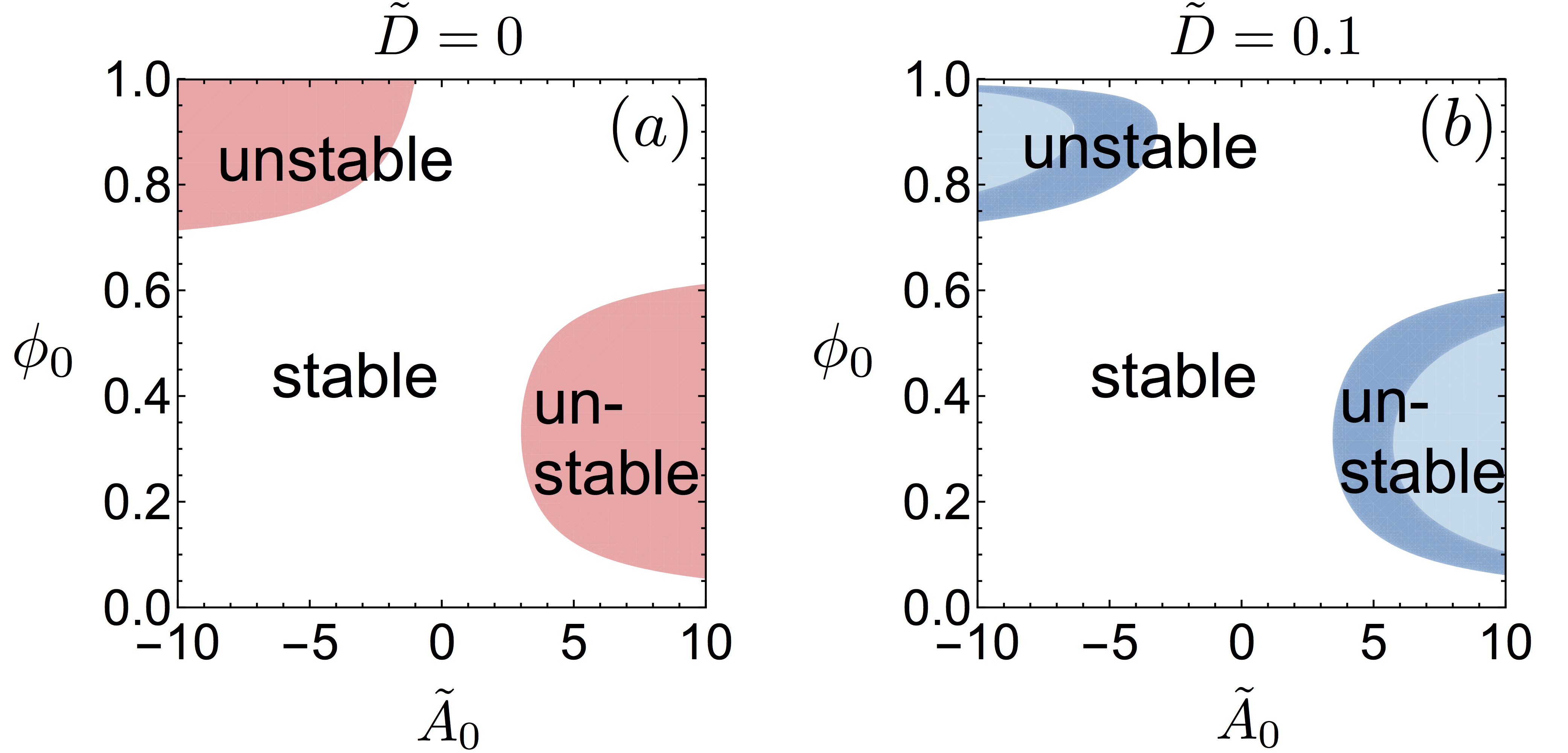
Figure S1: Stability diagrams indicating the parameter regimes where the homogeneous base state is stable or unstable for the case of an asymmetric choice of activity, ${A}^{(2)}=0$ and ${A}^{(1)}={A}_{0}\phi_{0}(1-\phi_{0})$ with $\tilde{{A}}_{0}={A}_{0}/\lambda$, and (a) $\tilde{D}=0$ and (b) $\tilde{D}=0.1$. The colored regions depict $\Re(\omega_{+})>0$. Dark and light blue correspond to $\Im(\omega_{k})\neq 0$ for all $q$, or for a finite waveband, respectively.

III Growth rates as a function of wavenumber for different parameters

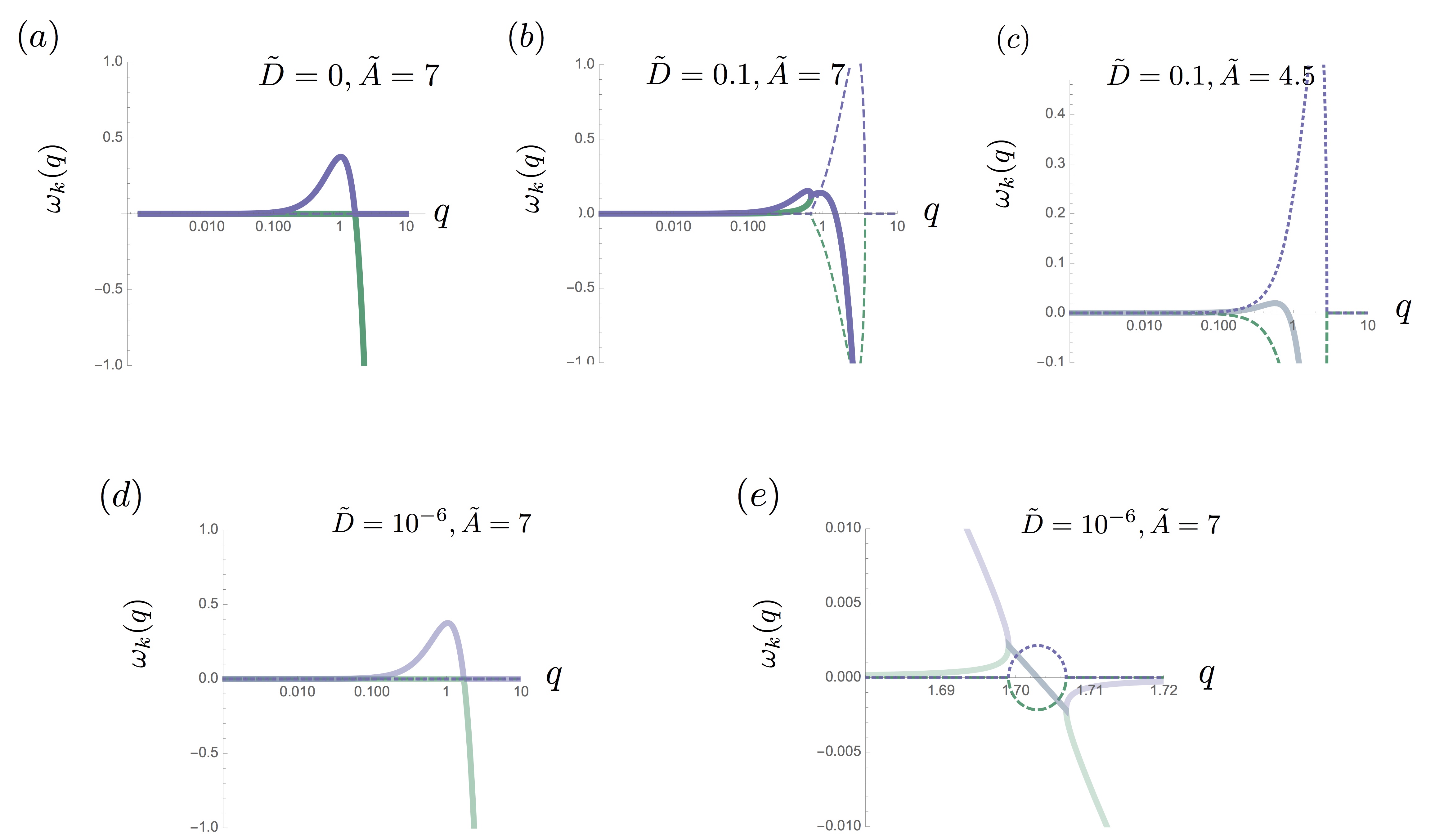
Figure S2: Growth rate $\omega_{k}(q)$ as a function of wavenumber for different parameters for our model one-dimensional model discussed in the main text. Solid lines indicate the real part of the growth rate, $\Re[\omega_{k}(q)]$, while the dashed lines correspond to the imaginary part, $\Im[\omega_{k}(q)]$. Parameters are $\phi_{0}=0.35$ and the remaining parameters are shown on each plot. (a) For $\tilde{D}=0$, the growth rate of the largest growing mode, $\omega_{+}(q)$ (purple), is real for all wavenumbers indicating a non-oscillatory growth of modes. (b) As the diffusivity $\tilde{D}$ increases, the growth rate becomes real for large $q$ but there remains a complex growth rate for a finite waveband at larger wavenumbers (light blue region in the phase diagram, main text, Fig. 2b). (c) Close to the transition where the instability vanishes (here we have decreased $\tilde{A}$ relative to (b)), the growth rate is complex for all wavenumbers (dark blue region in the phase diagram, main text, Fig. 2b). (d) However, deeply in the region of the phase diagram where the instability occurs, the width of the real waveband (as shown in (b)) decreases to zero as the diffusivity approaches zero. (e) This behavior is nicely visible in the wavenumber zoom-in corresponding to (d).

IV Details of numerical implementation

IV.1 Dynamical equations considered in the numerical studies

For our numerical studies we consider a biphasic mixture of a fluid (f) and solid-like (s) phase. Each phase $(i)$ is described by the hydrodynamic variables: velocity $v^{(i)}_{\alpha}$, volume fraction $\phi^{(i)}$ and displacement $u^{(i)}_{\alpha}$ with $\partial_{t}u^{(i)}_{\alpha}=v^{(i)}_{\alpha}$. For the numerical integration of the dynamical equations we introduce an inertia term on the left hand side of Eqs. (2a) and (2b) (main text) to make the numerical implementation straightforward (time evolution is easier than the force balance constraint). However, the quantitative influence on the solutions is expected to be negligible if the mass density $\rho$ is small enough . The full non-linear equations for the active biphasic system considered in the numerical studies read

$$\partial_{t}\phi =-\partial_{\alpha}\left(\phi v^{\text{s}}_{\alpha}\right)+D\partial_{\alpha}^{2}\phi\,,$$ (S10a)

$$0 =\partial_{\alpha}\left[\phi\,v^{\text{s}}_{\alpha}+\left(1-\phi\right)v^{\text{f}}_{\alpha}\right]\,,$$ (S10b)

$$\partial_{t}u_{\alpha} =v^{\text{s}}_{\alpha}\,,$$ (S10c)

$$\rho\phi\partial_{t}v^{\text{s}}_{\alpha} =\partial_{\beta}\left(\phi\sigma_{\alpha\beta}^{\text{s}}\right)-\phi\partial_{\alpha}p+\Gamma_{0}\phi(1-\phi)\left(v^{\text{f}}_{\alpha}-v^{\text{s}}_{\alpha}\right)\,,$$ (S10d)

$$\rho(1-\phi)\partial_{t}v^{\text{f}}_{\alpha} =\partial_{\beta}\left((1-\phi)\sigma_{\alpha\beta}^{\text{f}}\right)-(1-\phi)\partial_{\alpha}p-\Gamma_{0}\phi(1-\phi)\left(v^{\text{f}}_{\alpha}-v^{\text{s}}_{\alpha}\right)\,,$$ (S10e)

where $p$ denotes the pressure ensuring the incompressibility condition Eq. (S10b). The stress tensors of the solid (s) and fluid (f) phases are

$$\sigma^{\text{s}}_{\alpha\beta}= \lambda\,\delta_{\alpha\beta}\partial_{\gamma}u_{\gamma}+G\left(\partial_{\alpha}u_{\beta}+\partial_{\beta}u_{\alpha}\right)$$ (S11)

$$+ \bar{\lambda}\,\delta_{\alpha\beta}\partial_{\gamma}v^{\text{s}}_{\gamma}+\eta\left(\partial_{\alpha}v^{\text{s}}_{\beta}+\partial_{\beta}v^{\text{s}}_{\alpha}\right)+{A}_{0}\left[\left(\phi-\phi_{0}\right)-a\left(\phi-\phi_{0}\right)^{3}\right]\delta_{\alpha\beta}\,,$$

$$\sigma^{\text{f}}_{\alpha\beta} =0\,,$$ (S12)

where $\lambda$ is the first Lamé parameter and $G=\lambda(1-2\nu)/(2\nu)$ is the shear modulus, and $\nu$ denotes the Poisson ratio. Moreover, $\bar{\lambda}$ is the bulk viscosity and $\eta$ is the shear viscosity. The second viscosity $\zeta=\bar{\lambda}+2\eta/3$. We used the choice of the activity function given in Eq. (S8). For the fluid phase we neglected contributions proportional to velocity gradients because they are expected to be small on scales above the size of the solid pores. In addition, the solid viscosities typically exceeds the fluid viscosities by several orders of magnitude.

We rescale length and time as $x\to\ell\cdot x$ with $\ell=\sqrt{\bar{\lambda}/\Gamma_{0}}$, and $t\to(\ell/v_{0})\cdot t$, and consider a velocity rescaling $v^{(i)}_{\alpha}\to v_{\alpha}^{(i)}\cdot v_{0}$. The dimensional pressure and stress are $p\to p\cdot\lambda$ and $\sigma_{\alpha\beta}^{(i)}\to\sigma_{\alpha\beta}^{(i)}\cdot\lambda$. After this rescaling there are five dimensionless parameters in more than one dimension, namely $\tilde{A}_{0}={{A}_{0}}/\lambda$,$\tilde{D}=D/(\ell v_{0})$, $\tilde{G}=G/\lambda$, ${V}=v_{0}\bar{\lambda}/(\lambda\ell)=v_{0}\sqrt{\Gamma_{0}\bar{\lambda}}/\lambda$, and $\tilde{\eta}=V\eta/\bar{\lambda}$. In one dimension the two shear parameters ($\tilde{G}$, $\tilde{\eta}$) do not exist leading to three parameters. In the main text we considered the special case where the velocity scale $V=1$ leaving us with two non-dimensional parameters, namely the activity amplitude $\tilde{A}_{0}$ and the diffusivity $\tilde{D}$.

The dimensionless equations used for numerical discretization are

$$\partial_{t}\phi =-\partial_{\alpha}\left(\phi v^{\text{s}}_{\alpha}\right)+\tilde{D}\partial_{\alpha}^{2}\phi\,,$$ (S13a)

$$0 =\partial_{\alpha}\left[\phi\,v^{\text{s}}_{\alpha}+\left(1-\phi\right)v^{\text{f}}_{\alpha}\right]\,,$$ (S13b)

$$\partial_{t}u_{\alpha} =v^{\text{s}}_{\alpha}\,,$$ (S13c)

$$\hat{\rho}\phi\partial_{t}v^{\text{s}}_{\alpha} =\partial_{\beta}\left(\phi\sigma_{\alpha\beta}^{\text{s}}\right)-\phi\partial_{\alpha}p+\phi(1-\phi)\left(v^{\text{f}}_{\alpha}-v^{\text{s}}_{\alpha}\right)\,,$$ (S13d)

$$\hat{\rho}(1-\phi)\partial_{t}v^{\text{f}}_{\alpha} =-(1-\phi)\partial_{\alpha}p-V\,\phi(1-\phi)\left(v^{\text{f}}_{\alpha}-v^{\text{s}}_{\alpha}\right)\,,$$ (S13e)

where the dimensionless mass density is $\hat{\rho}=\rho v_{0}^{2}/\lambda$.

IV.2 Numerical methods used to solve dynamical equations in two dimensions

In the numerical integration we consider periodic boundary conditions. The two-dimensional simulations are performed with a custom C++ code and use an $N\times N$ grid for non-dimensional system size $(L/\ell)\times(L/\ell)$, where $\ell=\sqrt{\bar{\lambda}/\Gamma_{0}}$ is the unit length and $L$ is the system size. The spatial derivatives are discretized using second-order finite-differences. The time derivatives are discretized by an Euler scheme with a time increment of $\Delta t$ and a discrete time $t=n\cdot\Delta t$, where $n$ denotes the $n$-th time step.

In two dimensions, the essential step in the numerical integration is the calculation of the pressure in a way that the incompressibility holds (Eq. (S13b)). To this end, we apply a variant of Chorin’s projection method as used in the integration of the incompressible Navier–Stokes equations chorin68 . This method amounts to splitting the integration of Eqs. (S13d) and (S13e) into three parts. The first part calculates intermediate velocities $v^{\text{s},*}_{\alpha}$ and $v^{\text{f},*}_{\alpha}$ by neglecting the pressure gradient and relaxing the incompressibility constraint. These velocities are then used in the second part to compute the pressure via solving a Poisson problem. In the final part, the pressure is employed to project the velocities to satisfy the incompressibility constraint.

The first part of the projection step can thus be written as

$$\hat{\rho}\frac{v^{\text{s},*}_{\alpha}-v^{\text{s}}_{\alpha}(n)}{\Delta t} =\phi(n)^{-1}\partial_{\beta}\left(\phi(n)\sigma_{\alpha\beta}^{\text{s}}(n)\right)+V\,\left(1-\phi\left(n\right)\right)\left(v^{\text{f}}_{\alpha}(n)-v^{\text{s}}_{\alpha}(n)\right)\,,$$ (S14a)

$$\hat{\rho}\frac{v^{\text{f},*}_{\alpha}-v^{\text{f}}_{\alpha}(n)}{\Delta t} =-V\,\phi(n)\left(v^{\text{f}}_{\alpha}(n)-v^{\text{s}}_{\alpha}(n)\right)\,.$$ (S14b)

The second step can be derived by writing down the third step of the projection method,

$$\hat{\rho}\frac{v^{\text{s}}_{\alpha}(n+1)-v^{\text{s},*}_{\alpha}}{\Delta t} =-\partial_{\alpha}p(n+1)\,,$$ (S15a)

$$\hat{\rho}\frac{v^{\text{f}}_{\alpha}(n+1)-v^{\text{f},*}_{\alpha}}{\Delta t} =-\partial_{\alpha}p(n+1)\,.$$ (S15b)

The third step requires the knowledge of the pressure $p(n+1)$ at time step $n+1$ and computes the incompressible velocities $v^{\text{s}}_{\alpha}(n+1)$ and $v^{\text{f}}_{\alpha}(n+1)$ at time step $n+1$. The pressure is computed in the second step. Since $v^{\text{s}}_{\alpha}(n+1)$ and $v^{\text{f}}_{\alpha}(n+1)$ obey the incompressibility condition, multiplying Eq. (S15a) by $\phi(n)$ and Eq. (S15b) by $(1-\phi(n))$, and adding up both equations, applying the divergence and using the incompressibility condition for the incompressible velocities (Eq. (S13b)), we find

$$\partial_{\alpha}^{2}p(n+1) =\frac{\hat{\rho}}{\Delta t}\partial_{\alpha}\left[\phi(n)\,v^{\text{s},*}_{\alpha}+\left(1-\phi\left(n\right)\right)\,v^{\text{f},*}_{\alpha}\right]\,.$$ (S16)

The equation above represents the second step of the projection step. It is an elliptic problem, and is solved using a custom C++ implementation of the geometric multigrid method. Solving this equation gives the pressure $p(n+1)$, which is required in the third steps as described above.

$\phi_{0}$	$\tilde{D}$	$\tilde{A}_{0}$	$\nu$	$V$	$\tilde{\eta}$	$\hat{\rho}$	$a$
$0.5$	$0.005$–$5$	$0$–$10$	$0.48$ ($\tilde{G}\approx 0.0417$)	0.06	$0.02$	$0.02$	$20$

Table S1: A list of fixed parameters used to numerically solve Eq. (S17) in two spatial dimensions with the solid stress tensor given in Eq. (S11). For the numerical results please refer to main text, Fig. 3 and movies Sec. V.

In summary, given the fields $\phi(n)$, $v^{\text{s}}_{\alpha}(n)$, $v^{\text{f}}_{\alpha}(n)$ and $u_{\alpha}(n)$ at time step $n$, the full projection based algorithm in time is

$$\hat{\rho}\frac{v^{\text{s},*}_{\alpha}-v^{\text{s}}_{\alpha}(n)}{\Delta t} =\phi(n)^{-1}\partial_{\beta}\left(\phi(n)\sigma_{\alpha\beta}^{\text{s}}(n)\right)+V\,\left(1-\phi\left(n\right)\right)\left(v^{\text{f}}_{\alpha}(n)-v^{\text{s}}_{\alpha}(n)\right)\,,$$ (S17a)

$$\hat{\rho}\frac{v^{\text{f},*}_{\alpha}-v^{\text{f}}_{\alpha}(n)}{\Delta t} =-V\,\phi(n)\left(v^{\text{f}}_{\alpha}(n)-v^{\text{s}}_{\alpha}(n)\right)\,,$$ (S17b)

$$\partial_{\alpha}^{2}p(n+1) =\frac{\hat{\rho}}{\Delta t}\partial_{\alpha}\left[\phi(n)\,v^{\text{s},*}_{\alpha}+\left(1-\phi\left(n\right)\right)\,v^{\text{f},*}_{\alpha}\right]\,,$$ (S17c)

$$\hat{\rho}\frac{v^{\text{s}}_{\alpha}(n+1)-v^{\text{s},*}_{\alpha}}{\Delta t} =-\partial_{\alpha}p(n+1)\,,$$ (S17d)

$$\hat{\rho}\frac{v^{\text{f}}_{\alpha}(n+1)-v^{\text{f},*}_{\alpha}}{\Delta t} =-\partial_{\alpha}p(n+1)\,,$$ (S17e)

$$\frac{\phi(n+1)-\phi(n)}{\Delta t} =-\partial_{\alpha}\left(\phi(n)v^{\text{s}}_{\alpha}(n)\right)+\tilde{D}\partial_{\alpha}^{2}\phi(n)\,,$$ (S17f)

$$\frac{u_{\alpha}(n+1)-u_{\alpha}(n)}{\Delta t} =v^{\text{s}}_{\alpha}(n)\,.$$ (S17g)

The spatial derivatives are implemented using a second-order finite difference discretization (not shown). Parameters for the integration in two spatial dimensions are given in Table S1.

IV.3 Numerical solution of dynamical equations in one dimensions

In one dimension, the projection steps are not necessary since the incompressibility condition (Eq. (S13b)) implies a linear relationship between the velocities. With appropriate boundary conditions, $v^{f}=-v^{s}\phi/\left(1-\phi\right)$. Therefore, the pressure is determined and can be substituted. For the one-dimensional studies we considered a velocity scale $V=1$ for simplicity, leading to

$$\partial_{t}\phi =-\partial_{x}(\phi v)+\tilde{D}\partial_{x}^{2}\phi\,,$$ (S18a)

$$\partial_{t}u =v\,,$$ (S18b)

$$\hat{\rho}\frac{\phi}{1-\phi}\partial_{t}v =\partial_{x}\left(\phi\partial_{x}u\right)+\partial_{x}\left(\phi\partial_{x}v\right)+\phi({A}/\lambda)\,\partial_{x}\phi-\frac{\phi}{1-\phi}v^{\text{s}}\,,$$ (S18c)

where we abbreviated $v=v^{s}$ and ${A}(\phi)$ denotes the differential activity (main text, Eq. (3c)). We verified our one-dimensional results by our implementation as outlined above with the results obtained from a spectral based solver (XMDS2 dennis2013xmds2 ) and a finite element solver (Comsol Multiphysics^® software comsol ). The movies in 1D were rendered using the Comsol software.

V Movie description

We attached two movies for the one-dimensional (1D) equations (S18), and two for the two-dimensional (2D) equations (S17). If not stated below, parameters are given in Table S1.

• 1D: oscillating dynamics and collective motion. $\tilde{D}=0.4$, $\phi_{0}=0.5$, $\tilde{A}_{0}=6$, duration $T_{\text{}}=500$, $L/\ell=50$, grid points $N=500$.

• 1D: drifting domains undergoing fusion and break-up. $\tilde{D}=0.005$, $\phi_{0}=0.5$, $\tilde{A}_{0}=10$, duration $T_{\text{}}=250$, $L/\ell=50$, grid points $N=500$.

• 2D: pulsatory-type of dynamics. $\tilde{D}=0.4$, $\phi_{0}=0.5$, $\tilde{A}_{0}=6$, duration $T_{\text{}}=100$, $L/\ell=10$, grid points $N=256$.

• 2D: drifting domains undergoing fusion and break-up. $\tilde{D}=0.005$, $\phi_{0}=0.5$, $\tilde{A}_{0}=10$, duration $T_{\text{}}=100$, $L/\ell=10$, grid points $N=256$.

References

- (1) V. Schaller et al., Nature 467, 73 (2010).
- (2) C. Dombrowski et al., Phys. Rev. Lett. 93, 098103 (2004).
- (3) H. P. Zhang, A. Be’er, E.-L. Florin, and H. L. Swinney, Proc. Natl. Acad. Sci. USA 107, 13626 (2010).
- (4) C. A. Weber et al., Phys. Rev. Lett. 110, 208001 (2013).
- (5) F. Backouche, L. Haviv, D. Groswasser, and A. Bernheim-Groswasser, Physical Biology 3, 264 (2006).
- (6) A. Kudrolli, G. Lumay, D. Volfson, and L. S. Tsimring, Phys. Rev. Lett. 100, 058001 (2008).
- (7) Y. Sumino et al., Nature 483, 448 (2012).
- (8) V. Schaller et al., Proc. Natl. Acad. Sci. USA 108, 19183 (2011).
- (9) M. Mori et al., Current Biology 21, 606 (2011).
- (10) P. J. Foster, S. F rthauer, M. J. Shelley, and D. J. Needleman, eLife 4, e10837 (2015).
- (11) M. Rauzi, P.-F. Lenne, and T. Lecuit, Nature 468, 1110 (2010).
- (12) J. S. Bois, F. Jülicher, and S. W. Grill, Physical review letters 106, 028103 (2011).
- (13) J. Toner, Phys. Rev. E 86, 031918 (2012).
- (14) J. Prost, F. Jülicher, and J. Joanny, Nature Physics 11, 111 (2015).
- (15) I. S. Aranson and L. S. Tsimring, Phys. Rev. E 71, 050901 (2005).
- (16) E. Bertin, M. Droz, and G. Grégoire, J. Phys. A 42, 445001 (2009).
- (17) C. A. Weber, F. Thüroff, and E. Frey, New Journal of Physics 15, 045014 (2013).
- (18) F. Thüroff, C. A. Weber, and E. Frey, Phys. Rev. Lett. 111, 190601 (2013).
- (19) M. Barna and L. Niswander, Developmental Cell 12, 931 (2007).
- (20) J. M. Tabler, C. P. Rice, K. J. Liu, and J. B. Wallingford, Developmental Biology 417, 4 (2016).
- (21) A. C. Martin et al., The Journal of Cell Biology (2010).
- (22) P. M. Bendix et al., Biophysical Journal 94, 3126 (2008).
- (23) E. Moeendarbary et al., Nature materials 12, 253 (2013).
- (24) M. Radszuweit, S. Alonso, H. Engel, and M. Bär, Phys. Rev. Lett. 110, 138102 (2013).
- (25) M. Radszuweit, H. Engel, and M. Bär, PloS one 9, e99220 (2014).
- (26) J. Skotheim and L. Mahadevan, Proceedings of the Royal Society of London A: Mathematical, Physical and Engineering Sciences 460, 1995 (2004).
- (27) D. A. Drew, Annual review of fluid mechanics 15, 261 (1983).
- (28) J. P. Keener, S. Sircar, and A. L. Fogelson, SIAM Journal on Applied Mathematics 71, 854 (2011).
- (29) M. Doi, Journal of the Physical Society of Japan 78, 052001 (2009).
- (30) H. Tanaka, Physical review letters 71, 3158 (1993).
- (31) H. Tanaka, Journal of Physics: Condensed Matter 12, R207 (2000).
- (32) See Supplemental Material for videos and more information at http://link.aps.org/supplemental/… .
- (33) S. Barry and M. Holmes, IMA journal of applied mathematics 66, 175 (2001).
- (34) S. C. Cowin and L. Cardoso, Mechanics of Materials 44, 47 (2012).
- (35) The osmotic pressure can also be absorbed into a renormalized activity, which only shifts the transition to larger activities.
- (36) M. Spiegelman and D. McKenzie, Earth and Planetary Science Letters 83, 137 (1987).
- (37) N. Cogan, M. Donahue, and M. Whidden, Physical Review E 86, 056204 (2012).
- (38) S. Asakura and F. Oosawa, The Journal of Chemical Physics 22, 1255 (1954).
- (39) L. Onsager, Annals of the New York Academy of Sciences 51, 627 (1949).
- (40) P. J. Flory, The Journal of chemical physics 10, 51 (1942).
- (41) M. L. Huggins, The Journal of Physical Chemistry 46, 151 (1942).
- (42) M. S. Steinberg, Journal of Experimental Zoology 173, 395 (1970).
- (43) Specifically, the influence on the numerical integration of the added inertia terms are negligible if .
- (44) A. J. Chorin, Mathematics of Computation 22, 745 (1968).
- (45) G. R. Dennis, J. J. Hope, and M. T. Johnsson, Computer Physics Communications 184, 201 (2013).
- (46) COMSOL Multiphysics® v. 5.0. www.comsol.com. COMSOL AB, Stockholm, Sweden.